Abstract
This study introduces an innovative approach leveraging physics-informed neural networks (PINNs) for the efficient computation of blood flows at the boundaries of a four-vessel junction formed by a Fontan procedure. The methodology incorporates a 3D mesh generation technique based on the parameterization of the junction’s geometry, coupled with an advanced physically regularized neural network architecture. Synthetic datasets are generated through stationary 3D Navier–Stokes simulations within immobile boundaries, offering a precise alternative to resource-intensive computations. A comparative analysis of standard grid sampling and Latin hypercube sampling data generation methods is conducted, resulting in datasets comprising and samples, respectively. The following two families of feed-forward neural networks (FFNNs) are then compared: the conventional “black-box” approach using mean squared error (MSE) and a physically informed FFNN employing a physically regularized loss function (PRLF), incorporating mass conservation law. The study demonstrates that combining PRLF with Latin hypercube sampling enables the rapid minimization of relative error (RE) when using a smaller dataset, achieving a relative error value of on the test set. This approach offers a viable alternative to resource-intensive simulations, showcasing potential applications in patient-specific 1D network models of hemodynamics.
Keywords:
physics-informed neural networks; blood flow dynamics; computational hemodynamics; 3d mesh generation; Latin hypercube sampling; physically regularized loss function; cardiovascular diseases MSC:
92B20; 76Z05
1. Introduction
The blood flow dynamics in human vascular connections are critical for simulating hemodynamics in the presence of cardiovascular diseases and for devising effective treatment strategies. An accurate estimation of the blood flow parameters, such as pressures and flows, in these complex regions is important for informed clinical decision-making based on numerical simulations. The intricate interplay between various hemodynamic factors and the complexity of blood flow, especially in scenarios like the Fontan operation, pose challenges to an accurate estimation.
Palliative surgery is performed on patients with congenital heart disease (CHD). Conventionally, the first stage of palliative surgery involves the creation of a systemic-pulmonary shunt at birth to prepare the lung bed for subsequent operations. The second stage is the creation of a bidirectional cavopulmonary anastomosis (BCPA), which is the Glen operation. In the Glen operation, the trunk of the lung is separated from the heart and the superior vena cava is sutured to the pulmonary artery. The total cavopulmonary connection (TCPC), also known as the Fontan operation, is the final stage. This is considered to be a highly effective technique for diverting blood from the inferior vena cava to the pulmonary arteries; however, despite surgical correction, the complication rate remains high, and patient quality of life is often poor. A model-based understanding of the Fontan circulation and optimizing the Fontan operation can improve the prognosis for real patients [1].
3D models of blood flow allow clinicians to test a variety of vessel configurations and flow conditions. They allow the minimization of pulmonary and TCPC resistance, the energy dissipation in the TCPC, balance the hepatic and total flow distribution between the right and left lungs, and avoid regions with excessive or low wall shear stress. Local three-dimensional blood flow modeling is often used to solve such problems [2,3]. The junction of the inferior and superior vena cava (IVC and SVC) and the left and right pulmonary artery (LPA and RPA) forms the domain of integration. A fast evaluation of hemodynamic parameters without solving complex Navier–Stokes equations is desirable.
In the recent past, the convergence of deep learning and computational fluid dynamics has demonstrated considerable promise in tackling the aforementioned challenges [4]. Researchers have explored the use of physically informed neural networks (PINNs) to address the gap between intricate physical phenomena and data-driven predictive models. The key advantage of PINNs lies in their ability to integrate prior knowledge of the fundamental physical laws that govern fluid flow. This feature empowers the development of robust models capable of effectively handling complex vascular geometries.
In [5], PINN was developed to estimate aortic hemodynamics using dimensionless Navier–Stokes equations and the continuity equation for additional physical regularization. In [6], cerebral hemodynamics were estimated using PINN. Neural networks were trained in such a way as to satisfy the conservation of mass and momentum at all junction points in the arterial tree.
In this paper, we explore the use of PINNs for the estimation of blood flow parameters in a human vascular junction after the Fontan procedure. The emphasis is on creating an integrated methodology that combines data generation techniques with advanced neural network architectures. Following a successful training phase, the neural network demonstrates the capability to operate without demanding substantial computational resources during application.
We describe the process of training a physically regularized neural network. It starts with the creation of synthetic datasets using different sampling methods (standard grid sampling and Latin hypercube sampling (LHS)) First, a parametric set of 3D meshes was generated on the basis of the GMSH library [7]. The physiologic ranges of the radii and angles at the junction of the four vessels are considered. Next, the 3D simulations of blood flow were conducted for each geometry, employing stationary Navier–Stokes equations with fixed boundaries within a computational domain that represents rigid (immobile) vessel walls. The input parameters consist of the mean pressure values at the inflow and outflow boundaries, while the output parameters comprise the mean flow values at these boundaries. Ideally, the training dataset should be derived from real patient data, necessitating a substantial volume of measurements across a broad spectrum of parameter values—an undertaking that is challenging with current equipment capabilities. To address this challenge, our approach involves the generation of synthetic data through a 3D stationary Navier–Stokes finite element solver.
Furthermore, we explore different loss functions, the standard “black-box” approach (mean squared error (MSE)) and physically regularized loss function (PRLF). We propose a PRLF implementation, which includes a mass conservation condition. The adaptive moment estimation (Adam) algorithm of optimization is used for loss function minimization [8]. We achieve an average relative error of for MSE. The integration of the PRLF with LHS facilitated convergence on a reduced dataset, yielding a diminished relative error of approximately on the test dataset.
The paper is organized as follows: In Section 2.1, we describe the methods of dataset generation, including the parametric mesh generation and a brief mathematical formalization for the flow simulations. In Section 3, we describe the general design of the developed neural networks and introduce MSE and PRLF. In Section 4, we present the Adam optimization technique and discuss the hyperparameter optimization problem. Section 5 contains the experimental results. The conclusions are presented in Section 6.
2. Dataset Generation
Our objective is to predict the average flow values at the boundaries of a 3D vascular junction involving the convergence of four vessels, as illustrated in Figure 1. To achieve this, we adopt a neural network approach, formulating the problem as a multi-variable regression task. The junction geometry is parameterized by the angles formed between the vessels and the radii of each vessel, as detailed in Section 2.1. In Section 2.2, we establish the pressure boundary conditions at each inflow and outflow boundary to facilitate the computation of incompressible flows. This is achieved by solving the stationary Navier–Stokes equations within a domain with fixed boundaries. In Section 2.3, we explicate the LHS method, which, in conjunction with standard grid search sampling, will be employed to generate the definitive sets of geometries and pressures for training a neural network.
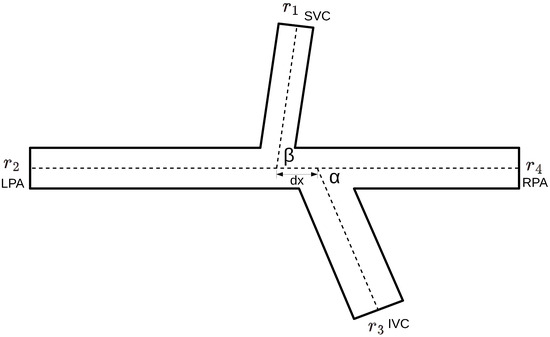
Figure 1.
Schematic representation of the junction of the following four vessels: inferior vena cava (IVC), superior vena cava (SVC), left pulmonary artery (LPA), and right pulmonary artery (RPA). The corresponding vessel radii (), vessel junction angles (), and the distance between the centers of the superior and inferior vena cava () are marked on the scheme.
2.1. Parametric Generation of 3D Domain for a Junction of Four Vessels
To automate the construction of 3D meshes for the junction of four vessels, we have developed a parametric mesh generation software leveraging the GMSH [7] library. It is assumed that all vessels lie in a single plane. As inputs, the generator takes two angles between the vessels at the junction, along with the lengths and radii of the four segments forming the junction region (refer to Figure 2 left). The computational domain is defined as the union of several cylindrical tubes (see Figure 2 left). A uniform mesh is constructed inside the domain (see Figure 2 right).
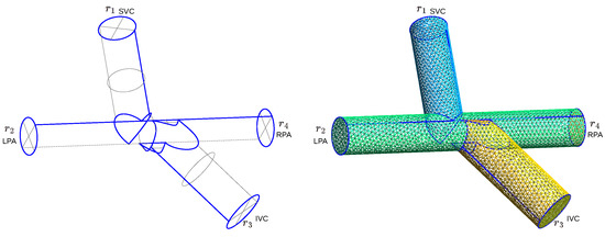
Figure 2.
Illustration of the mesh generation algorithm for creating a 3D geometric model and computational domain of a four vessels junction: left—placement of marks on the mesh surfaces, right—construction of an unstructured mesh from tubular segments.
Following mesh construction, additional mesh optimization from the Ani3D [9] package is applied. This optimization involves the repartitioning of tetrahedra, with all vertices lying on the boundary of the region, contributing to the stability of numerical methods for computing flow in the junction.
2.2. Calculation of Hydrodynamic Parameters
The blood is assumed to be a viscous, incompressible fluid with viscosity = 0.04 cm2s−1 and density = 1 g/cm3. The 3D domain of the junction area of four vessels (see Figure 2 right) with boundary is composed of rigid walls , two inlets , and two outlets . The blood flow in is described by the stationary 3D Navier–Stokes equations as follows:
where p is the pressure, is the velocity vector field, and is the outward normal vector to the boundary surface. On the immobile side wall, we assume a no-slip and no-penetration boundary condition. At the inlets and the outlets , we set the average pressures , , , and as the boundary conditions.
The LBB-stable Taylor–Hood (P2/P1) finite element method is used for the approximation of (1). The multifrontal sparse direct solver MUMPS [10] based on the exact factorization of the matrix is applied for solving the resulted system of equations. The model has been extensively presented in [11]. The solution of the discrete nonlinear problem results in the velocity vector field and the pressure field in the computational domain. The average blood flows q at the boundaries and are calculated for further neural network training as follows:
2.3. Latin Hypercube Sampling
To systematically explore the parameter space and enhance the diversity of our dataset, we use the LHS [12] method. LHS is a statistical technique designed to ensure a more uniform and representative sampling of the multidimensional parameter space. In particular, we hypothesize that this approach will be valuable in capturing a wide range of physiological variations in vascular junction geometry.
Let be the parameter space defined by the angles between vessels, and the distance between the IVC and SVC centers and radii of the four segments form the junction region. For each parameter, LHS guarantees a proportional and stratified sampling. Consider N samples drawn from , denoted as . These samples are obtained such that the marginal distribution of each parameter is uniformly represented, and the correlations between the parameters are minimized.
In Section 5, we provide a visual comparison of the dataset that is obtained by the standard grid search and the dataset that is obtained by the LHS method.
3. Design of the Neural Network
In this section, we develop a FFNN designed to predict the values of the input and output flows (, , , and ) based on the geometry of the junction and the pressure values (, , , and ).
FFNNs [13] represent a commonly utilized class of neural networks. In FFNNs, data flows unidirectionally from inputs to outputs without feedback, making it suitable for solving classification and regression tasks.
A typical FFNN implementation comprises a series of layers, with each layer containing a set of neurons (refer to Figure 3). The neurons in a layer are connected to the neurons in the preceding and succeeding layers. Input data traverses the network, and each neuron performs computations based on its input values, activation function, and connection weights. The output is then transmitted to the subsequent layer, and this process continues until reaching the output layer, generating the final output.
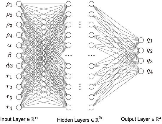
Figure 3.
The structure of the designed FFNN. is the number of hidden layers, is the number of neurons in the hidden layers, and k is the index of FFNN implementation.
The specification of a FFNN involves determining the number of layers and neurons, selecting an activation function for each neuron, defining a loss function that relies on the connection weights between neurons, implementing a drop-out algorithm for potential random disconnection of certain neurons from the network, and establishing an optimization procedure to minimize the loss function with respect to the weights. Each of these components is elaborated upon in the subsequent sections.
Determining the appropriate size of a neural network, which encompasses the number of layers and neurons in each layer, is a critical task that requires manual consideration based on the specific task and available data. A network that is too small may yield subpar results, while an excessively large one can exhibit overtraining on known data and perform poorly on new data.
For our task, the input and output layer sizes are known, with the number of neurons in the first layer corresponding to the input parameters (eleven), and the last layer matching the number of predicted parameters (four). Determining the size of hidden layers presents a challenge, and we explore two approaches. One method involves an experimental selection based on numerous numerical experiments and computational resources, especially when both training and test datasets are available. Alternatively, an initial overestimated size can be chosen, and neurons are selectively removed during training based on weights or randomly.
In this study, we employ the drop-out algorithm, as described in [14], which involves randomly removing neurons. The probability of removal is manually set, which allows the network to avoid over-adaptation to the input data and mitigates overtraining. This approach promotes the development of more robust features and enhances the generalization ability of the neural network.
Before transmitting data to the subsequent layer, the neural network utilizes an activation function on the weighted sum of signals originating from the neurons of the preceding layer. Commonly employed activation functions include the sigmoid function [15], which is defined as follows:
and the rectified linear unit (ReLU) [16]
where x is the sum of the outputs from the neurons of the previous layer.
Several studies [17,18] have indicated that the choice of activation function is seldom a decisive factor in training FFNN. Both (3) and (4) yield satisfactory results. However, research [19] has highlighted the advantages of the rectified linear unit (ReLU) activation function (4) over the sigmoidal activation function (3). ReLU-based FFNNs demand fewer computational resources during the training phase, enabling more efficient numerical experiments. Consequently, we opt for ReLU in the design of all our FFNN implementations.
The critical consideration in designing FFNN involves selecting a suitable loss (error) function. The loss function is denoted as , where represents the vector of predicted values, and is the vector of true values.
For a loss function to be effective, it must adhere to the following criteria [20]:
- Non-negativity: The error function’s value cannot be negative, as it serves as a measure of the disparity between the predicted and actual values;
- Continuity: The error function needs to be continuous to ensure a smooth relationship between the input data and model error;
- Differentiability: Since most optimization algorithms rely on derivatives, the error function must be differentiable concerning the model parameters.
In this work, we consider and compare the following two error functions: MSE and PRLF, which we also refer as PINN.
MSE is defined as follows:
where n is the number of rows in the dataset, are predicted values, and are true values.
MSE functions are commonly used in standard black-box machine learning techniques without prior knowledge of the system structure and behavior. In addition to MSE we exploit PRLF, which is an extension of MSE as follows:
where PhysLoss is a physical component.
In practice, we apply supplementary regularization, imposing penalties on the model for deviating from physical constraints. This methodology is known as physical regularization, and neural networks incorporating this technique are commonly known as PINNs [21].
We enforce the following singular physical constraint on the blood flow within a junction of four vessels: the preservation of mass condition.
Finally, we state the physical component of the loss function as follows:
where n is the number of rows in the dataset and is the weight of the conservation law component, are predicted values of the i-th flow
We employed two distinct error metrics, namely, relative error (RE) and R-squared (R2), to comprehensively assess the performance of our neural network during the training process. RE measures the average percentage deviation between the true target values and the predicted values , providing a relative measure of the model’s accuracy across all data points. On the other hand, R2 quantifies the goodness-of-fit of the model by assessing the proportion of the variability in the target variables explained by the model. A higher R2 value indicates a better fit, with 1 denoting a perfect fit and 0 indicating no explanatory power. The RE and R2 defined as follows:
where represents the observed target values, , represents the predicted values, and is the mean of the observed values. By incorporating both RE and R2, we obtained a comprehensive understanding of the model’s accuracy, capturing both the relative deviation and the overall explanatory power.
4. Neural Network Training
The neural network training relies on the error backpropagation algorithm [22], enabling the optimization of network parameters to minimize prediction errors. During training, input data are introduced to the network’s input layer, and the information is forwarded through its layers of neurons. The output values are then compared to the expected correct answers, and an error function is computed to quantify the disparity between the predictions and the target values; subsequently, the error backpropagation phase commences. The neurons in the final layer receive information about the error, and, utilizing the gradient descent algorithm, adjust their weights to diminish the error. This error propagation process recurs backward through the network, influencing the weights of the neurons in preceding layers. This iterative process continues for each training example or mini-batch (a subset of data used for training) until the model reaches optimal weights. Various implementations of the backpropagation algorithm exist, with Adam [8] being considered among the most effective at the time of writing this paper.
Adam, short for adaptive moment estimation [8], represents an optimization algorithm designed to dynamically adjust the learning rate for individual parameters by considering the first and second moments of the loss function gradient. This adaptive approach facilitates rapid convergence to the optimal solution and mitigates the influence of data noise on model training. The Adam algorithm can be succinctly described as follows:
where t is iteration number, are attenuation coefficients for the moments, which are selected manually, and are the first and second moments of the gradients at the iteration t, which are set to 0 at the first iteration, and are adjusted values of the moments at the iteration t, is vector of neural network weights at the iteration t, is gradient of , with respect to the loss function , is learning rate, which is selected manually and controls how much the weights of the neural network change at each iteration, and is a small number for numerical stability.
Hyperparameters [23] are integral settings for FFNN, defining its structure and functionality while influencing the network’s capacity to learn and generalize to unseen data. This set encompasses parameters like the number of hidden layers, the quantity of neurons within these layers, the weight assigned to the physical component in the error function, the batch size, the method for initializing neural network weights, and the learning rate for the optimization algorithm.
Optimizing hyperparameters during training through gradient-based methods is unfeasible. Instead, various heuristic approaches are employed to determine suitable values. In this study, we employ the grid search method for hyperparameter selection. Finally, the hyperparameters of the FFNN are given in Table 1.

Table 1.
Hyperparameters of the FFNN.
5. Results
The dataset for neural network training was created basing on the junction of four vessels with various angles, radii, and boundary pressures. The length of all segments was set to 7 cm. The radii of the SVC (), LPA (), and RPA () ranged from 0.7 to 2.3 cm. At each iteration of mesh generation, these radii were equal to each other. The radius of the IVC () ranged from to for each value of . The distance between the centers of the SVC and IVC () ranged from 0 to for each combination of values and . Angles ranged from 60 to 120 degrees. The pressures ranged from −100 to 100 Pa.
Next, we used the following two different approaches to generate the meshes: generating data on a grid with an uniform step size, and LHS In the first case, the following steps were used: , and were ranged with step 0.4. The range step was chosen so that 2 different values between and were obtained. The range step was chosen so that two different values between 0 to were obtained. The angles were ranged with step 30. The pressures were ranged with step 50. In the end, 180 grids were generated. On each grid, 64 iterations of flow calculations were performed. As a result, samples of data were generated by the first method.
In the second case, the Latin hypercube sampling method was used. When using this method, the required number of final samples and parameter intervals are specified. We generated 100 meshes using this method. Then, also using the Latin hypercube method, 50 pressure combinations were generated for each mesh to calculate the flows. Finally, samples of data were generated by the second method. In contrast to the conventional grid search method, Latin hypercube sampling (LHS) was anticipated to augment the diversity within our dataset. To elucidate the distinctions between the acquired datasets, we employed principal component analysis (PCA) [24] to reduce their dimensionality. The visual representation (refer to Figure 4) substantiates the superior dataset diversity achieved through the utilization of LHS.
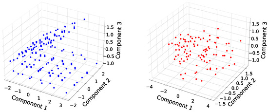
Figure 4.
Comparison of datasets obtained using different sampling methods: left—dataset obtained by standard grid search, right—dataset obtained using LHS.
The random subset of the dataset was used for training the FFNNs and the remaining was used for testing. The technical stack for FFNNs training is shown in Table 2.
Table 2.
Parameters of the technical stack.
The construction of the ultimate algorithm entails a two-step experimental process. Initially, we will assess neural networks trained on both a standard dataset and a LHS dataset, utilizing the MSE loss function for training. Subsequently, a similar comparative analysis will be conducted employing the PINN error function. Throughout these investigations, the inter-neuronal connections are characterized by a ReLU transfer function, and the optimization task is executed using the Adam algorithm. Ultimately, the evaluation of all the trained models will be based on the comparison of RE and R2 values extracted from the best training iterations.
In the initial phase, a distinct superiority of the neural network trained on the standard dataset over its counterpart trained on the LHS dataset is evident. Figure 5 illustrates the convergence trajectories of these FFNNs. The RE value of the neural network trained on the standard dataset converges to a range of 8–10%, whereas the RE value of the neural network trained on the LHS dataset converges to 10–13%. Both neural networks converge to a high R2 value (Figure 5 bottom left, bottom right), approaching unity; however, the convergence rate of the neural network trained on the standard dataset is notably higher. At this juncture, the interim inference can be made that, when utilizing MSE as the loss function, the convergence of the neural network trained on the standard dataset surpasses that of the neural network trained on the LHS dataset. It is plausible that achieving comparable convergence with MSE would necessitate augmenting the size of the LHS dataset to at least match that of the standard dataset.
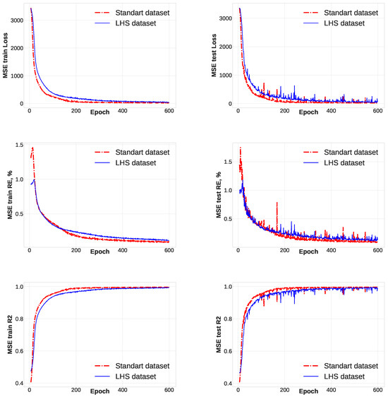
Figure 5.
Convergence of the classic FFNN with MSE: upper left—PRLF on training set, upper right—PRLF on test set, middle left—RE on training set, middle right—RE on test set, bottom left—R2 on training set, bottom right—R2 on test set.
During the second phase, we observe a comparable convergence pattern in both the neural network trained on the standard dataset and the one trained on the LHS dataset. Figure 6 illustrates the convergence trajectories of these FFNNs. Both networks converge to RE values within the range of 6–7%, indicating a satisfactory convergence. Furthermore, the R2 value approximating 1 (Figure 6 bottom left, bottom right) signifies that both neural networks accurately capture the target variables variance in both datasets. These observations are corroborated by the test dataset, as depicted in Figure 6 upper right, middle left. Notably, the neural network trained on the LHS dataset exhibits fewer outliers in the RE convergence graph. Simultaneously, a significant reduction in PRLF and RE is observed after the 200th iteration in the neural network trained on the standard dataset. This suggests that the neural network finds it more straightforward to adapt to the samples from the standard dataset compared to those from the LHS dataset. In essence, the utilization of the LHS dataset serves as an additional regularization method for the neural network, expanding the parameter space. Despite the LHS dataset being almost half the size of the standard dataset, the neural network achieves a satisfactory RE value, indicating the superiority of the LHS dataset generation approach in this step.
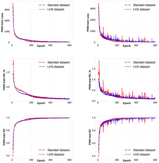
Figure 6.
Convergence of the classic FFNN with PRLF: upper left—PRLF on training set, upper right—PRLF on test set, middle left—RE on training set, middle right—RE on test set, bottom left—R2 on training set, bottom right—R2 on test set.
Finally, we performed a comparison of the trained neural networks’ performance based on the optimal RE values on the test set in Table 3. Given that all neural networks achieved exceptionally high R2 values, we excluded this metric from the comparative analysis.
Table 3.
RE of trained models on the test set.
6. Conclusions
In this study, we introduce a novel approach for efficiently computing the flows at the boundaries of a four-vessel junction using the physics-informed neural network (PINN) methodology. Our methodology involves the development of a 3D mesh generation technique, which is based on the parameterization of the four vessels’ junction through the geometry of the connected vessels. This is coupled with an advanced physically regularized neural network architecture. The synthetic dataset is generated through the solution of 3D stationary Navier–Stokes equations within the generated domains, where the boundaries remain immobile. The boundary conditions are set by specifying pressures at the inlets and outlets, and the flow is computed as the outcome of the simulations. This innovative approach integrates mesh generation, physically informed neural networks, and synthetic dataset generation to efficiently compute flows at complex vascular junctions.
We conducted a comparative analysis of two data generation approaches, namely, standard grid sampling and Latin hypercube sampling. The resulting datasets comprised and samples, respectively, encompassing a diverse range of physiologically plausible cases. Subsequently, we compared the following two families of FFNNs: one employing the conventional “black-box” methodology with MSE and the other adopting a physically informed FFNN approach with a physically regularized loss function (PRLF). In this context, we introduced the PRLF implementation, which incorporates the mass conservation law. The analysis revealed that the combination of PRLF with the Latin hypercube sampling (LHS) method enables the rapid minimization of the relative error (RE) using a smaller dataset. This amalgamation of methods facilitated the attainment of a relative error value of on the test set.
The extensive utilization of 3D models necessitates substantial computing resources. Our approach offers a viable alternative by replacing these resource-intensive simulations with a rapid and precise algorithm. The developed technique holds potential for establishing boundary conditions in patient-specific 1D network models of hemodynamics in the future [25,26,27].
Further validation with a broader range of parameters is necessary. In this study, the true optimization of FFNN hyperparameters was not explicitly conducted. Nevertheless, undertaking such optimization represents a crucial step in enhancing our methodology. For instance, this process could lead to the elimination of less significant neurons, whose contributions do not substantially impact the final predicted values.
In the mesh generation phase, we make the assumption that all segments of the four-vessel junction lie within a single plane. This assumption remains valid for our study, given that the influence of the gravity field is not considered. However, a more limiting assumption is the adoption of a stationary incompressible flow model with immobile boundaries. The incorporation of an unsteady flow model or even fluid–structure interaction simulations has the potential to significantly enhance our approach. It is imperative to validate the developed technique with data obtained from real patients. This step is essential for ensuring the reliability and applicability of the methodology in clinical scenarios.
The findings of this research showcase the substantial potential of PINNs in accurately predicting blood flow parameters. Furthermore, the study highlights the capability of PINNs in constructing innovative computational techniques for conducting patient-specific hemodynamic simulations. The simple practical application of our PINN model based on PRLF, is the analysis of the blood flow parameters in the junction of the vessels after the Fontan procedure.
Author Contributions
Conceptualization, T.D. and S.S.; methodology, A.I. and S.S.; software, A.I., T.D. and A.D.; validation, A.I. and T.D.; data curation, A.I.; writing—original draft preparation, A.I. and S.S.; writing—review and editing, A.I., T.D., A.D. and S.S.; visualization, A.I. and A.D.; supervision, S.S. All authors have read and agreed to the published version of the manuscript.
Funding
This work has been supported by the Russian Science Foundation, grant number 21-71-30023.
Data Availability Statement
Dataset available on request from the authors.
Conflicts of Interest
The authors declare no conflicts of interest.
Abbreviations
The following abbreviations are used in this manuscript:
| BCPA | Bidirectional cavopulmonary anastomosis |
| CHD | Congenital heart disease |
| FFNN | Feed-forward neural networks |
| IVC | Inferior vena cava |
| LHS | Latin hypercube sampling |
| LPA | Left pulmonary artery |
| MSE | Mean squared error |
| PINN | Physics-informed neural network |
| RE | Relative error |
| RPA | Right pulmonary artery |
| PRLF | Physically regularized loss function |
| R2 | R-squared error |
| SVC | Superior vena cava |
| TCPC | Total cavopulmonary connection |
References
- De Zélicourt, D.; Kurtcuoglu, V. Patient-Specific Surgical Planning, Where Do We Stand? The Example of the Fontan Procedure. Ann. Biomed. Eng. 2015, 44, 174–186. [Google Scholar] [CrossRef]
- Siallagan, D.; Loke, Y.H.; Olivieri, L.; Opfermann, J.; Ong, C.; De Zélicourt, D.; Petrou, A.; Daners, M.; Kurtcuoglu, V.; Meboldt, M.; et al. Virtual surgical planning, flow simulation, and 3-dimensional electrospinning of patient-specific grafts to optimize Fontan hemodynamics. J. Thorac. Cardiovasc. Surg. 2018, 155, 1734–1742. [Google Scholar] [CrossRef]
- Yang, W.; Chan, F.; Reddy, V.; Marsden, A.; Feinstein, J. Flow simulations and validation for the first cohort of patients undergoing the Y-graft Fontan procedure. J. Thorac. Cardiovasc. Surg. 2015, 149, 247–255. [Google Scholar] [CrossRef]
- Kutz, J. Deep learning in fluid dynamics. J. Fluid Mech. 2017, 814, 1–4. [Google Scholar] [CrossRef]
- Du, M.; Zhang, C.; Xie, S.; Pu, F.; Zhang, D.; Li, D. Investigation on aortic hemodynamics based on physics-informed neural network. Math. Biosci. Eng. 2023, 20, 11545–11567. [Google Scholar] [CrossRef] [PubMed]
- Sarabian, M.; Babaee, H.; Laksari, K. Physics-Informed Neural Networks for Brain Hemodynamic Predictions Using Medical Imaging. IEEE Trans. Med. Imaging 2022, 41, 2285–2303. [Google Scholar] [CrossRef] [PubMed]
- Geuzaine, C.; Remacle, J. Gmsh: A 3-D Finite Element Mesh Generator with Built-in Pre- and Post-Processing Facilities. Int. J. Numer. Methods Eng. 2009, 79, 1309–1331. [Google Scholar] [CrossRef]
- Kingma, D.; Adam, J.B. A Method for Stochastic Optimization. In Proceedings of the 2nd International Conference on Learning Representations, ICLR 2014, Banff, AB, Canada, 14–16 April 2014. [Google Scholar]
- Vassilevski, Y.; Lipnikov, K. An adaptive algorithm for quasioptimal mesh generation. Comp. Math. Math. Phys. 1999, 39, 1468–1486. [Google Scholar]
- Amestoy, P.R.; Duff, I.S.; L’Excellent, J.Y.; Koster, J. A Fully Asynchronous Multifrontal Solver Using Distributed Dynamic Scheduling. SIAM J. Matrix Anal. Appl. 2001, 23, 15–41. [Google Scholar] [CrossRef]
- Vassilevski, Y.; Olshanskii, M.; Simakov, S.; Kolobov, A.; Danilov, A. Personalized Computational Hemodynamics. Models, Methods, and Applications for Vascular Surgery and Antitumor Therapy; Academic Press: Cambridge, MA, USA, 2020. [Google Scholar]
- Helton, J.; Davis, F. Latin hypercube sampling and the propagation of uncertainty in analyses of complex systems. Reliab. Eng. Syst. Saf. 2003, 81, 23–69. [Google Scholar] [CrossRef]
- Bebis, G.; Georgiopoulos, M. Feed-forward neural networks. IEEE Potentials 1994, 13, 27–31. [Google Scholar] [CrossRef]
- Srivastava, N.; Hinton, G.; Krizhevsky, A.; Sutskever, I.; Salakhutdinov, R. Dropout: A Simple Way to Prevent Neural Networks from Overfitting. J. Mach. Learn. Res. 2014, 15, 1929–1958. [Google Scholar]
- Sridhar, N. The generalized sigmoid activation function: Competitive supervised learning. Inf. Sci. 1997, 99, 69–82. [Google Scholar] [CrossRef]
- Nair, V.; Hinton, G. Rectified Linear Units Improve Restricted Boltzmann Machines. In Proceedings of the International Conference on Machine Learning, Haifa, Israel, 21–24 June 2010. [Google Scholar]
- Pretorius, A.; Barnard, E.; Davel, M. ReLU and sigmoidal activation functions. In Fundamentals of Artificial Intelligence Research; Springer: Berlin/Heidelberg, Germany, 2019. [Google Scholar]
- Nwankpa, C.; Ijomah, W.; Gachagan, A.; Marshall, S. Activation Functions: Comparison of trends in Practice and Research for Deep Learning. arXiv 2018, arXiv:1811.03378. [Google Scholar]
- Krizhevsky, A.; Sutskever, I.; Hinton, G. ImageNet classification with deep convolutional neural networks. Commun. ACM 2012, 60, 84–90. [Google Scholar] [CrossRef]
- Goodfellow, I.; Bengio, Y.; Courville, A. Deep Learning; Adaptive Computation and Machine Learning; MIT Press: Cambridge, MA, USA, 2016. [Google Scholar]
- Amin, M.; Meidani, H. Physics-Informed Regularization of Deep Neural Networks. arXiv 2018, arXiv:1810.05547v1. [Google Scholar]
- Rojas, R. The Backpropagation Algorithm. In Neural Networks: A Systematic Introduction; Springer: Berlin/Heidelberg, Germany, 1996; pp. 149–182. [Google Scholar] [CrossRef]
- Claesen, M.; De Moor, B. Hyperparameter Search in Machine Learning. arXiv 2015, arXiv:1502.02127. [Google Scholar]
- Maćkiewicz, A.; Ratajczak, W. Principal Components Analysis (PCA). Comput. Geosci. 1993, 19, 303–342. [Google Scholar] [CrossRef]
- Müller, L.O.; Watanabe, S.M.; Toro, E.F.; Feijóo, R.A.; Blanco, P.J. An anatomically detailed arterial-venous network model. Cerebral and coronary circulation. Front. Physiol. 2023, 14, 1162391. [Google Scholar] [CrossRef] [PubMed]
- Simakov, S.S.; Gamilov, T.M.; Liang, F.; Gognieva, D.G.; Gappoeva, M.K.; Kopylov, P.Y. Numerical evaluation of the effectiveness of coronary revascularization. Russ. J. Numer. Anal. Math. Model. 2021, 36, 303–312. [Google Scholar] [CrossRef]
- Gognieva, D.; Mitina, Y.; Gamilov, T.; Pryamonosov, R.; Vassilevski, Y.; Simakov, S.; Liang, F.; Ternovoy, S.; Serova, N.; Tebenkova, E.; et al. Noninvasive Assessment of the Fractional Flow Reserve with the CT FFRc 1D Method: Final Results of a Pilot Study. Glob. Heart 2021, 16, 1. [Google Scholar] [CrossRef] [PubMed]
Disclaimer/Publisher’s Note: The statements, opinions and data contained in all publications are solely those of the individual author(s) and contributor(s) and not of MDPI and/or the editor(s). MDPI and/or the editor(s) disclaim responsibility for any injury to people or property resulting from any ideas, methods, instructions or products referred to in the content. |
© 2024 by the authors. Licensee MDPI, Basel, Switzerland. This article is an open access article distributed under the terms and conditions of the Creative Commons Attribution (CC BY) license (https://creativecommons.org/licenses/by/4.0/).