On Barrier Binary Options in the Telegraph-like Financial Market Model

Abstract

The article continues the study of the market model based on jump-telegraph processes. It is assumed that the price of a risky asset follows the stochastic exponential of a piecewise linear process, equipped with jumps that occur at the moments of a pattern change. In this case, the standard option pricing formula was derived previously, while exotic options for this model have not yet been explored. Within this framework, we are developing procedures for pricing binary barrier options. This article concerns the “cash-(at hit)-or-nothing” binary barrier option. The main tools of this analysis are methods developed for first-pass probabilities. Some known results related to the ruin probabilities follow directly from these settings.

1. Introduction

The stochastic approach to modelling nature and society is quite common and useful for understanding the world. In general, various types of Wiener/Levy processes are used for these purposes, which, it is also generally recognised, have a number of serious drawbacks. Among other things, these models are characterised by an infinite propagation velocity, which contradicts the generally accepted naive idea. Another disadvantage is the singularity and unlimited variation of paths. In this article, our goal is to develop a mathematical methodology and the application of such improvements that avoid these shortcomings. Our approach is based on the so-called telegraph processes.

In the traditional setting [1,2], the telegraph process describes the position $X\left(t\right)$ at time $t,t\ge 0,$ of a particle, which moves on the line with constant velocities $\pm 1$ alternating at the random time epochs of an underlying Poisson process. Namely, $X\left(t\right)=\xi {\int }_0^t{(-1)}^{N\left(s\right)}\mathrm{d}s$, where $\xi =\pm 1/2$ is the (random) initial direction and $N=N\left(t\right)$ is a counting Poisson process; $\xi$ and N are mutually independent.

Recently, various generalisations of this process have been proposed, also aimed at financial applications. First, the process X can be set as an inhomogeneous with different particle speeds and different rates of regime switching, which is reasonable since the symmetric case is very restrictive. Secondly, a purely jump component with deterministic [3] and independent random jumps [4] that occur when switching velocities is added to the telegraph process. At the same time, it is worth noting that the addition of jumps is necessary not only to better match the model to real markets but also for purely methodological reasons since the model of a continuous telegraph process leads to arbitrage opportunities.

To make the presentation more precise, consider a two-state Markov process $ϵ=ϵ\left(t\right)\in \{0,1\}$, which is controlled by alternating switching rates ${\lambda }_0$ and ${\lambda }_1$. Let $N=N\left(t\right)$ be an inhomogeneous Poisson process counting switchings. Consider a sequence of mutually independent random variables ${\left\{Y_n\right\}}_{n\ge 1}$ independent of ${ϵ}^{}$.

Consider a jump-telegraph process $X\left(t\right)+J\left(t\right),t\ge 0,$ with constant alternating velocities $c_0,c_1,$ and random jumps $Y_n$:

$$X\left(t\right)={\int }_0^t{c}_{ϵ\left(s\right)}\mathrm{d}s,J\left(t\right)=\sum _{n=1}^{N\left(t\right)}{Y}_n.$$

In this paper, we continue to explore the one-asset market model with dynamics $S\left(t\right)$ of a risky asset price, which follows a stochastic exponential of $X+J$:

$$S\left(t\right)=S_0{\mathcal{E}}_t(X+J)=S_{0}exp\left({\int }_0^t{c}_{{ϵ}^{(}s)}\mathrm{d}s\right)·\prod _{n=1}^{N\left(t\right)}(1+Y_n).$$

This approach to market modelling substitutes a Wiener process in the classic Black–Scholes model with a telegraph process with jumps, which better fits the traditional view of price evolution.

This idea is now well understood. It should be noted that this model continues to develop in various directions, see a comprehensive review in [5], where the main attention is paid to option pricing within this model.

Note that the standard call option pricing formula has the same structure as the classic Black–Scholes formula. Meanwhile, exotic options are much less studied. This paper is focused on the “cash-(at hit)-or-nothing barrier binary option”, which involves the payment of a unit of capital when the level $x,$ fixed in advance, is first reached.

2. Market Model and Measure Transform

Let $ϵ=ϵ\left(t\right)\in \{0,1\},t\ge 0,$ be a Markov process with two states, defined on a complete probability space $(\mathsf{\Omega },\mathcal{F},\mathbb{P})$ and switching at random times ${\left\{{\tau }_n\right\}}_{n\ge 1},{\tau }_0=0,$ controlled by two alternating rates ${\lambda }_0$ and ${\lambda }_1$.

In this setting, a piecewise linear stochastic process $X\left(t\right)={\int }_0^t{c}_{{ϵ}^{(}u)}\mathrm{d}u, t\ge 0,$ can be regarded as an asymmetric integrated telegraph process. The two pairs of parameters $(c_0,{\lambda }_0),(c_1,{\lambda }_1)$, $c_0\ge c_1$, completely determine the distribution of $X\left(t\right).$ For any $t>0$, the distribution of $X\left(t\right)$ is supported on $[c_{1}t,c_{0}t]$ with atoms at the extreme points:

$$\mathbb{P}\{X\left(t\right)=c_{0}t|ϵ\left(0\right)=0\}={\mathrm{e}}^{-{\lambda }_{0}t},\mathbb{P}\{X\left(t\right)=c_{1}t|ϵ\left(0\right)=1\}={\mathrm{e}}^{-{\lambda }_{1}t},$$

(1)

and, for $c_{1}t<x<c_{0}t,$

$$\begin{array}{l}\mathbb{P}\{X\left(t\right)\in \mathrm{d}x|ϵ\left(0\right)=0\}/\mathrm{d}x\\ =\left. [{\lambda }_0{I}_0\left(2\sqrt{{\lambda }_0{\lambda }_1{\xi }_0(x,t){\xi }_1(x,t)}\right)+{\left({\lambda }_0{\lambda }_1\frac{{\xi }_0(x,t)}{{\xi }_1(x,t)}\right)}^{1/2}{I}_1\left(2\sqrt{{\lambda }_0{\lambda }_1{\xi }_0(x,t){\xi }_1(x,t)}\right)\right]\theta (x,t),\\ \mathbb{P}\{X\left(t\right)\in \mathrm{d}x|ϵ\left(0\right)=1\}/\mathrm{d}x\\ =\left. [{\lambda }_1{I}_0\left(2\sqrt{{\lambda }_0{\lambda }_1{\xi }_0(x,t){\xi }_1(x,t)}\right)+{\left({\lambda }_0{\lambda }_1\frac{{\xi }_1(x,t)}{{\xi }_0(x,t)}\right)}^{1/2}{I}_1\left(2\sqrt{{\lambda }_0{\lambda }_1{\xi }_0(x,t){\xi }_1(x,t)}\right)\right]\theta (x,t).\end{array}$$

(2)

Here, ${\xi }_0(x,t)={\displaystyle \frac{x-c_{1}t}{c_0-c_1}},{\xi }_1(x,t)=t-{\xi }_0(x,t),0<{\xi }_0(x,t),{\xi }_1(x,t)<t,$

$$\theta (x,t)={\displaystyle \frac{exp(-{\lambda }_0{\xi }_0(x,t)-{\lambda }_1{\xi }_1(x,t))}{c_0-c_1}},$$

and $I_0(·),I_1(·)$ are modified Bessel functions, see, e.g., [5].

In search of a model without the disadvantages mentioned in the introduction, we will use the telegraph process instead of the Wiener process usually exploited for financial markets modelling. Note that simply replacing the Wiener process with a telegraph process of this form leads to arbitrage opportunities. This feature was not taken into account in the first attempts to construct such a generalisation of the Black–Scholes market model, where an integrated telegraph process was used instead of Brownian motion, see [6,7,8]. At the same time, these pioneering works are still interesting. For example, in article [7], stochastic order comparisons of price processes were presented, which later were not developed. Article [8] is devoted to some optimisation problems related to finding the optimal time to sell a stock, which also need to be developed.

Various ways have been suggested in the literature to avoid arbitrage, but the simplest and most natural is to add jumps after each speed switching. Here, we will focus on this issue.

Consider a compound Poisson process $J=J\left(t\right)={\sum }_{n=1}^{N\left(t\right)}{Y}_n$ with independent random jumps of the amplitudes $Y=Y_n,Y_n>-1$. Assume that the distributions $h_0$ and $h_1$ of the jump amplitudes $Y_n$ change alternately as the market state $ϵ=ϵ\left(t\right)$ switches.

We study a market model consisting of a single risky asset with a price $S\left(t\right),t\ge 0,$ which follows the ordinary stochastic equation

$$\mathrm{d}S\left(t\right)=S(t-)\mathrm{d}\left(X\left(t\right)+J\left(t\right)\right),t>0.$$

(3)

Integrating (3), we have a geometric jump-telegraph process of the form $S\left(t\right)=S_0{\mathcal{E}}_t\left(X+J\right),$ $t\ge 0.$ Here, ${\mathcal{E}}_t(·)$ is the stochastic (Doléans–Dade) exponential, so that $S\left(t\right)=S_0{\mathrm{e}}^{X\left(t\right)}{\kappa }_{N\left(t\right)},$ where ${\kappa }_{N\left(t\right)}={\prod }_{k=1}^{N\left(t\right)}(1+Y_n).$ See, for example, [9].

For simplicity, let the interest rates $r_0\ge 0$ and $r_1\ge 0$ be constant in each market state, so that the bond price is a geometric telegraph process,

$$B\left(t\right)=exp\left({\int }_0^t{r}_{{ϵ}^{(}s)}\mathrm{d}s\right),t\ge 0.$$

(4)

Thus, the discounted asset price, $B{\left(t\right)}^{-1}S\left(t\right),$ is again a geometric jump-telegraph process.

The martingale properties of such a model are characterised by the following well-known results.

Theorem 1.

Let $X+J$ be a jump-telegraph process.

(a)

The jump-telegraph process $X+J$ and its stochastic exponent $S\left(t\right)={\mathcal{E}}_t(X+J),$ $t\ge 0,$ are martingale if and only if

$$c_0+{\lambda }_0{y}_0=0,c_1+{\lambda }_1{y}_1=0.$$

(5)

Here, $y_0$ and $y_1$ are the average amplitudes of the jumps associated with states 0 and 1, respectively,

$$y_0={\mathbb{E}}_0\left[Y\right]={\int }_{-\infty }^{\infty }z{h}_0\left(\mathrm{d}z\right),y_1={\mathbb{E}}_1\left[Y\right]={\int }_{-\infty }^{\infty }z{h}_1\left(\mathrm{d}z\right).$$

(b)

For models (3)–(4), there is an equivalent martingale measure $\tilde{\mathbb{P}}$ if and only if there exists a pair of positive measurable functions ${\phi }_0,{\phi }_1$ such that

$$-r_0+c_0+{\int }_{-1}^{\infty }z{\phi }_0\left(z\right)h_0\left(\mathrm{d}z\right)=0,-r_1+c_1+{\int }_{-1}^{\infty }z{\phi }_1\left(z\right)h_1\left(\mathrm{d}z\right)=0.$$

(6)

Under the new measure $\tilde{\mathbb{P}},$ the Poisson rates ${\lambda }_i,i\in \{0,1\},$ are changed to

$${\lambda }_0^{\ast }={\int }_{-1}^{\infty }{\phi }_0\left(z\right)h_0\left(\mathrm{d}z\right),{\lambda }_1^{\ast }={\int }_{-1}^{\infty }{\phi }_1\left(z\right)h_1\left(\mathrm{d}z\right),$$

(7)

and the jump amplitudes are distributed as

$$h_i^{\ast }\left(\mathrm{d}z\right)=\frac{{\phi }_i\left(z\right)}{{\lambda }_i^{\ast }}{h}_i\left(\mathrm{d}z\right),i\in \{0,1\},$$

(8)

For the proof, see [4] (Theorem 2.2 and 3.1).

In particular, note that conditions (5) require that the average jump value be opposite to the current velocity direction.

Consider an option with a payoff $\mathcal{H}={\mathcal{H}}_{\tau }$ that occurs at time $\tau$. After the martingale measure $\tilde{\mathbb{P}}$ is chosen, the price of this option is given by a pair

$${\mathfrak{c}}_0={\mathbb{E}}_{\tilde{\mathbb{P}}}\left. [B{\left(\tau \right)}^{-1}{\mathcal{H}}_{\tau }\left|ϵ\right(0)=0\right],{\mathfrak{c}}_1={\mathbb{E}}_{\tilde{\mathbb{P}}}\left. [B{\left(\tau \right)}^{-1}{\mathcal{H}}_{\tau }\left|ϵ\right(0)=1\right].$$

In this paper, we are focused on the so-called binary barrier options in which the payoff $\mathcal{H}$ is either some fixed amount or nothing depending on the breakdown of the fixed threshold. See an overview of various binary barrier options and their pricing methods in [10].

3. Pricing “Cash-(At Hit)-or-Nothing Barrier Binary Option”

We are interested in pricing of the option in the simple case when the payoff is received at the moment the barrier x is breached. To be specific, let $S_0<x$.

Consider an option of getting 1 when the asset price exceeds the threshold $x,$ i.e., the option with a payoff function $\mathcal{H}\left(x\right)={\mathrm{𝟙}}_{\left\{{max}_{t>0}S\left(t\right)>x\right\}},$ where ${\mathrm{𝟙}}_A$ is the indicator of event A. It is assumed that the payoff is received at time

$$T\left(x\right)=inf\{t>0|S\left(t\right)>x\}$$

(9)

when the stock price $S\left(t\right)$, $t>0,$ reaches the barrier x for the first time. We assume that the interest rate r is strictly positive, since for $r=0$ the option price is always 1.

Let $\tilde{\mathbb{P}}$ be the martingale measure. The option price is given by a pair (depending on the state of the market at underwriting) of bond-discounted payoff expectations with respect to the martingale measure $\tilde{\mathbb{P}},$

$${\mathfrak{c}}_0={\mathbb{E}}_{\tilde{\mathbb{P}}}\left. [{\mathrm{e}}^{-rT\left(x\right)}\left|ϵ\right(0)=0\right],{\mathfrak{c}}_1={\mathbb{E}}_{\tilde{\mathbb{P}}}\left. [{\mathrm{e}}^{-rT\left(x\right)}\left|ϵ\right(0)=1\right].$$

(10)

By definition, $0\le {\varphi }_i\left(x\right)\le 1,\forall x$.

Note that the first time $T\left(x\right)$ when the stock price $S\left(t\right)$ reaches the threshold x coincides with the first passage time $\mathcal{T}\left(\overline{x}\right)$ of $X\left(t\right)+log\kappa \left(t\right)$ through the threshold $\overline{x}=log[x/S_0]$.

In what follows, we study the first passage time problem for the logarithm of the stock price. To get the answers for the market model (3) and (4), it suffices to modify the results obtained below by replacing $x\to \overline{x}=log(x/S_0)$.

3.1. “Bull Market” and Positive Threshold

We consider first the model with alternating positive trends $c_0>c_1>0,$ and negative jump amplitudes. This means that the bull market is correcting down at the switch points. The latter means that the alternating distributions $h_0$ and $h_1$ of $Y_n$-corrections to the rising market prices

$$S\left(t\right)=S_{0}exp\left(X\left(t\right)\right)·\prod _{n=1}^{N\left(t\right)}(1+Y_n)$$

are supported on the interval $(-1,0]$.

Let $\mathcal{T}\left(x\right)=T(log(x/S_0)$ denote the first passage time through the threshold $x,$ by the jump-telegraph process $X\left(t\right)+log\kappa \left(t\right).$ Since both velocities are positive, note that this process breaches the barrier x by continuously moving between jumps.

By conditioning on the first velocity switching, the following identities in law are valid,

$$\begin{gathered} {\mathcal{T}}_0\left(x\right)\stackrel{D}{=}\frac{x}{c_0}{\mathrm{𝟙}}_{\{\tau >x/c_0\}}+\left. [\tau +{\mathcal{T}}_1(x-c_0\tau -log(1+Y))\right]{\mathrm{𝟙}}_{\{\tau <x/c_0\}}, \\ {\mathcal{T}}_1\left(x\right)\stackrel{D}{=}\frac{x}{c_1}{\mathrm{𝟙}}_{\{\tau >x/c_1\}}+\left. [\tau +{\mathcal{T}}_0(x-c_1\tau -log(1+Y))\right]{\mathrm{𝟙}}_{\{\tau <x/c_1\}}, \end{gathered}$$

(11)

where $\tau$ is the holding time before the first jumping and Y is the first jump amplitude. Here, $“\stackrel{D}{=}”$ denotes the equality in distribution. We denote by ${\mathcal{T}}_i(·)$ the first passage time if the initial state $i,i\in \{0,1\},$ is given.

Let the interest rate $r=r_0=r_1$ be positive.

Applying (11) to the Laplace transforms

$${\varphi }_0\left(x\right)={\mathbb{E}}_{\tilde{\mathbb{P}}}\left. [{\mathrm{e}}^{-r\mathcal{T}\left(x\right)}\left|ϵ\right(0)=0\right],{\varphi }_1\left(x\right)={\mathbb{E}}_{\tilde{\mathbb{P}}}\left. [{\mathrm{e}}^{-r\mathcal{T}\left(x\right)}\left|ϵ\right(0)=1\right],$$

cf (10), we obtain a pair of coupled integral equations,

$$\begin{array}{cc}\hfill {\varphi }_0\left(x\right)={\mathrm{e}}^{-({\lambda }_0+r)x/c_0}+& {\int }_0^{x/c_0}{\lambda }_0{\mathrm{e}}^{-({\lambda }_0+r)t}\left({\int }_{-1}^0{\varphi }_1(x-c_{0}t-log(1+y))h_0\left(\mathrm{d}y\right)\right)\mathrm{d}t,\hfill \\ \hfill {\varphi }_1\left(x\right)={\mathrm{e}}^{-({\lambda }_1+r)x/c_1}+& {\int }_0^{x/c_1}{\lambda }_1{\mathrm{e}}^{-({\lambda }_1+r)t}\left({\int }_{-1}^0{\varphi }_0(x-c_{1}t-log(1+y))h_1\left(\mathrm{d}y\right)\right)\mathrm{d}t,\hfill \end{array}x>0.$$

(12)

Since $\mathcal{T}\left(x\right)\to 0$ a.s. for $x\downarrow 0,$ then ${\varphi }_0\left(0\right)={\varphi }_1\left(0\right)=1$. Further, since $\mathcal{T}\left(x\right)>x/c_0$ a.s., then ${\varphi }_0\left(x\right),{\varphi }_1\left(x\right)\to 0$ as $x\to +\infty$.

Equation (12) can be rewritten as equations in convolutions:

$$\begin{array}{c}{\varphi }_0\left(x\right)={\psi }_{{\beta }_0}\left(x\right)+\frac{{\lambda }_0}{c_0}{\psi }_{{\beta }_0}\ast (h_0\ast {\varphi }_1)\left(x\right),\\ {\varphi }_1\left(x\right)={\psi }_{{\beta }_1}\left(x\right)+\frac{{\lambda }_1}{c_1}{\psi }_{{\beta }_1}\ast (h_1\ast {\varphi }_0)\left(x\right),\end{array}x\ge 0,$$

(13)

where ${\psi }_{\beta }\left(x\right)=exp(-\beta x){\mathrm{𝟙}}_{\{x\ge 0\}}$, and

$$\begin{gathered} h\ast \varphi \left(x\right)={\int }_{-1}^0\varphi (x-log(1+y))h\left(\mathrm{d}y\right),{\psi }_{\beta }\ast \varphi \left(x\right)={\int }_0^x\varphi (x-y){\psi }_{\beta }\left(y\right)\mathrm{d}y; \\ {\beta }_0=\frac{r+{\lambda }_0}{c_0},{\beta }_1=\frac{r+{\lambda }_1}{c_1}. \end{gathered}$$

We hope that the use of some informal notations, when convolutions with a jump distribution and with a function are denoted in a similar way, will not cause misunderstandings.

The system of integral Equation (12) has a unique bounded solution [11]. To write this solution explicitly, note that ${\psi }_{\beta },$ is an eigenfunction of the convolution with measure $h(·),$

$$h\ast {\psi }_{\beta }\left(x\right)={\int }_{-1}^{0}exp\left(-\beta (x-log(1+y\left)\right)\right)h\left(\mathrm{d}y\right)=\widehat{h}\left(\beta \right){\psi }_{\beta }\left(x\right),x>0,$$

where

$$\widehat{h}\left(\beta \right)={\int }_{-1}^0{(1+y)}^{\beta }h\left(\mathrm{d}y\right)>0,$$

if the latter integral converges. Further,

$${\psi }_{\beta }\ast {\psi }_{\alpha }\left(x\right)={\int }_0^x{\mathrm{e}}^{-\alpha (x-y)}{\mathrm{e}}^{-\beta y}\mathrm{d}y=\frac{{\psi }_{\alpha }\left(x\right)-{\psi }_{\beta }\left(x\right)}{\beta -\alpha },\alpha \ne \beta .$$

We find a solution of (13) in the form

$$\overrightarrow{\varphi }\left(x\right)=({\varphi }_0\left(x\right), {\varphi }_1\left(x\right))=\sum _{n=0}^N{\psi }_{{\alpha }_n}\left(x\right){\overrightarrow{z}}_n,$$

(14)

with indefinite coefficients ${\overrightarrow{z}}_n=(A_n, B_n)$ and ${\alpha }_n,\mathrm{Re}{\alpha }_n>0,{\alpha }_n\ne {\beta }_0,{\beta }_1,n\in \{0,1,\dots ,N\}$.

Substituting this function into (13), we obtain the following algebraic system:

$$\begin{gathered} \sum _{n=0}^N{A}_n{\psi }_{{\alpha }_n}\left(x\right)={\psi }_{{\beta }_0}\left(x\right)+\sum _{n=0}^N\frac{{\lambda }_0{\widehat{h}}_0\left({\alpha }_n\right)/c_0}{{\beta }_0-{\alpha }_n}{B}_n\left. [{\psi }_{{\alpha }_n}\left(x\right)-{\psi }_{{\beta }_0}\left(x\right)\right], \\ \sum _{n=0}^N{B}_n{\psi }_{{\alpha }_n}\left(x\right)={\psi }_{{\beta }_1}\left(x\right)+\sum _{n=0}^N\frac{{\lambda }_1{\widehat{h}}_1\left({\alpha }_n\right)/c_1}{{\beta }_1-{\alpha }_n}{A}_n\left. [{\psi }_{{\alpha }_n}\left(x\right)-{\psi }_{{\beta }_1}\left(x\right)\right], \end{gathered}$$

(15)

which is equivalent to

$$\begin{array}{ccc}\hfill A_n=\frac{{\lambda }_0{\widehat{h}}_0\left({\alpha }_n\right)}{c_0({\beta }_0-{\alpha }_n)}{B}_n,& B_n=\frac{{\lambda }_1{\widehat{h}}_1\left({\alpha }_n\right)}{c_1({\beta }_1-{\alpha }_n)}{A}_n,\hfill & \\ \hfill & n\in \{0,1,\dots ,N\};\hfill & \end{array}$$

(16)

$$\begin{array}{cc}\hfill \sum _{n=0}^N{A}_n=1,& \sum _{n=0}^N{B}_n=1.\hfill \end{array}$$

(17)

From (16), it follows that $\alpha ={\alpha }_n$ are the positive roots of the algebraic equation

$${\lambda }_0{\lambda }_1{\widehat{h}}_0\left(\alpha \right){\widehat{h}}_1\left(\alpha \right)=c_0{c}_1(\alpha -{\beta }_0)(\alpha -{\beta }_1).$$

(18)

Notice that for a real positive $\alpha ,$ the value $\widehat{h}\left(\alpha \right)$ is real, $0<\widehat{h}\left(\alpha \right)<1,$ so if the interest rate is strictly positive, then

$$(c_0\alpha -{\lambda }_0-r)(c_1\alpha -{\lambda }_1-r){{|}_{\alpha =0}=({\lambda }_0+r)({\lambda }_1+r)>{\lambda }_0{\lambda }_1={\lambda }_0{\lambda }_1{\widehat{h}}_0\left(\alpha \right){\widehat{h}}_1\left(\alpha \right)|}_{\alpha =0}.$$

Therefore, since the function $\alpha \to \widehat{h}\left(\alpha \right)>0,\alpha \in (0,\infty ),$ is decreasing, Equation (18) always has exactly two positive roots, ${\alpha }_0,{\alpha }_1$, such that

$$0<{\alpha }_0<min\left({\beta }_0,{\beta }_1\right)\le max\left({\beta }_0,{\beta }_1\right)<{\alpha }_1.$$

Hence, the solution of system (13) is given by (14) with $N=1$. The explicit form of coefficients ${\overrightarrow{z}}_0$ and ${\overrightarrow{z}}_1$ follows from Equations (16)–(18):

$$\begin{array}{l}{A}_0=\frac{k_0(k_1-1)}{k_0{k}_1-1},A_1=\frac{k_0-1}{k_0{k}_1-1},B_0=\frac{k_1-1}{k_0{k}_1-1},B_1=\frac{k_1(k_0-1)}{k_0{k}_1-1},\mathrm{where}\\ k_0=\frac{{\lambda }_0{\widehat{h}}_0\left({\alpha }_0\right)}{c_0({\beta }_0-{\alpha }_0)}=\frac{c_1({\beta }_1-{\alpha }_0)}{{\lambda }_1{\widehat{h}}_1\left({\alpha }_0\right)},k_1=\frac{{\lambda }_1{\widehat{h}}_1\left({\alpha }_1\right)}{c_1({\beta }_1-{\alpha }_1)}=\frac{c_0({\beta }_0-{\alpha }_1)}{{\lambda }_0{\widehat{h}}_0\left({\alpha }_1\right)}.\end{array}$$

(19)

Example 1.

Consider the case of$c_0\ge c_1\ge 0$and identically distributed exponential downward jumps with

$$h_0\left(\mathrm{d}y\right)=h_1\left(\mathrm{d}y\right)=h\left(\mathrm{d}y\right)=b{(1+y)}^{b-1}{\mathrm{𝟙}}_{\{-1<y<0\}}\mathrm{d}y,b>0,$$

(20)

and let${\beta }_0={\beta }_1=\beta .$Notice that the distribution of jump$Y,-1<Y<0,$given by (20), corresponds to the exponential distribution of the r.v. $-log(1+Y),$

$$\mathbb{P}\{-log(1+Y)>x\}=\mathbb{P}\{Y<-1+{\mathrm{e}}^{-x}\}=exp(-bx),x>0.$$

Since

$${\widehat{h}}_0\left(\alpha \right)={\widehat{h}}_1\left(\alpha \right)={\int }_{-1}^0{(1+y)}^{\alpha }h\left(\mathrm{d}y\right)=b{\int }_{-1}^0{(1+y)}^{\alpha +b-1}\mathrm{d}y=\frac{b}{\alpha +b},$$

Equation (18) becomes

$${\lambda }_0{\lambda }_1\frac{b^2}{{(\alpha +b)}^2}=c_0{c}_1{(\alpha -\beta )}^2,$$

which splits into two quadratic equations that can be solved explicitly. The positive roots are

$${\alpha }_0=\frac{1}{2}\left(\beta -b+\sqrt{{(\beta +b)}^2-4a}\right)<\beta ,{\alpha }_1=\frac{1}{2}\left(\beta -b+\sqrt{{(\beta +b)}^2+4a}\right)>\beta ,$$

(21)

where $a=b\sqrt{{\displaystyle \frac{{\lambda }_0{\lambda }_1}{c_0{c}_1}}},$ and

$$({\alpha }_0-\beta )({\alpha }_0+b)=+a,({\alpha }_1-\beta )({\alpha }_1+b)=-a.$$

(22)

By virtue of (22),

$$\begin{gathered} k_0=\frac{{\lambda }_{0}b}{c_0(b+{\alpha }_0)(\beta -{\alpha }_0)}=\frac{{\lambda }_{0}b}{c_{0}a}=\sqrt{\frac{{\lambda }_0{c}_1}{{\lambda }_1{c}_0}}>0, \\ {k}_1=\frac{{\lambda }_{1}b}{c_0(b+{\alpha }_1)(\beta -{\alpha }_1)}=-\frac{{\lambda }_{1}b}{c_{1}a}=-\sqrt{\frac{{\lambda }_1{c}_0}{{\lambda }_0{c}_1}}<0, \end{gathered}$$

(23)

hence, $k_0{k}_1=-1$. Therefore, ${\varphi }_0\left(x\right)$ and ${\varphi }_1\left(x\right)$ are determined by (14) with coefficients (see (19))

$$A_0=\frac{1}{2}(1+k_0),A_1=\frac{1}{2}(1-k_0),B_0=\frac{1}{2}(1-k_1),B_1=\frac{1}{2}(1+k_1).$$

(24)

Notice that in the symmetric case with$\beta ={\lambda }_0/c_0={\lambda }_1/c_1$and a zero interest rate$r=0,$we have$k_0=1,k_1=-1.$ Since ${\alpha }_0{|}_{r=0}=\left(\beta -b\right){\mathrm{𝟙}}_{\{\beta \ge b\}},$ then (14) simplifies to

$${\varphi }_0\left(x\right)={\varphi }_1\left(x\right)=exp(-{\alpha }_{0}x)=\left\{\begin{array}{ll}exp\left(-(\beta -b)x\right),\hfill & if\beta >b,\hfill \\ 1,\hfill & \mathit{otherwise},\hfill \end{array}\right.$$

(25)

which coincides with known results, see [12].

The same follows for the Cramér–Lundberg model${\lambda }_0={\lambda }_1,c_0=c_1,r\ge 0$.

Further, by [13] (Formulas (2.2.5)–(18)), the inverse Laplace transform of the function

$$q\to exp(aq-a\sqrt{q^2-z^2})-1,q>z,$$

is given by

$$\frac{az}{\sqrt{t^2+2at}}{I}_1\left(z\sqrt{t^2+2at}\right),$$

where $I_1(·)$ denotes the modified Bessel function of the first order. Due to (21), the probability density function $p(t;x)$ of $T\left(x\right),p(t;x)={\mathcal{L}}_{q\to t}^{-1}\left(exp(-{\alpha }_0\left(q\right)x)\right)$ takes the form

$$p(t;x)={\mathrm{e}}^{-\lambda t}\left. [\delta \left(t-x/c\right)+\frac{x\sqrt{\lambda b}}{\sqrt{t(ct-x)}}{I}_1\left(2\sqrt{\lambda bt(ct-x)}\right)\right],t>-x/c,$$

where $\delta (·)$ is the Dirac delta-function, corresponding to movement without switching.

Generally speaking, the dynamics ${\varphi }_0$ and ${\varphi }_1$ of option prices are quite diverse. Some of numerical results based on (14), (18), and (19) for exponentially distributed downward jumps are shown in Figure 1, Figure 2 and Figure 3. Figure 2 shows two opposite behaviours of the option price. Panel (a) depicts the case when in state 0 the price experiences large and frequent jumps compared to small but rare ones (in state 1). In this case, ${\varphi }_1\left(x\right)\gg {\varphi }_0\left(x\right).$ Panel (b) shows the opposite case, where the risky asset price experiences large infrequent jumps (state 0) versus small but frequent jumps (state 1). In this case, ${\varphi }_0\left(x\right)>{\varphi }_1\left(x\right)$.

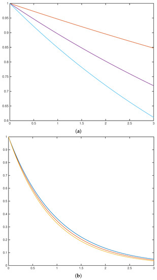
Figure 1. The option price ${\varphi }_0\left(x\right),0\le x\le 3$ for the interest rates $r=0.05/0.10/0.15$ (from top to bottom): (a) in the symmetric case, $c_0=c_1=1,{\lambda }_0={\lambda }_1=1,b_0=b_1=1,$ (here ${\varphi }_0={\varphi }_1$); (b) in the case $c_0=1, c_1=0.5,{\lambda }_0=1, {\lambda }_1=4,b_0=1, b_1=0.1$.

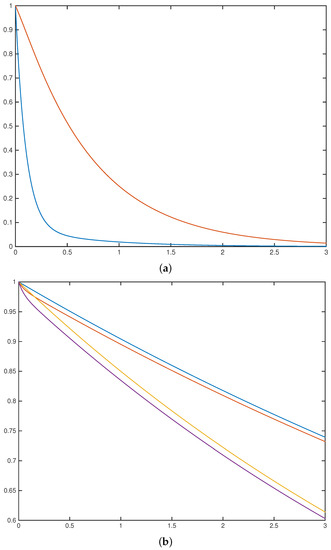
Figure 2. The option price ${\varphi }_0\left(x\right)$ and ${\varphi }_1\left(x\right),x>0,$ in two “opposite” cases. (a): $c_0=1, {\lambda }_0=10,$ $b_0=0.1$ and $c_1=0.1, {\lambda }_1=0.1, b_1=10.$ Interest rate $r=0.1$. Here, ${\varphi }_1\gg {\varphi }_0;$ (b): $c_0=1,$ ${\lambda }_0=0.1, b_0=0.1$, and $c_1=0.5, {\lambda }_1=10,$ $b_1=10,$ Two pairs of the curves correspond to different interest rates, $r=0.05$ (top pair of curves) and $r=0.1$ (lower pair of curves). In both cases, ${\varphi }_0\left(x\right)>{\varphi }_1\left(x\right)$.

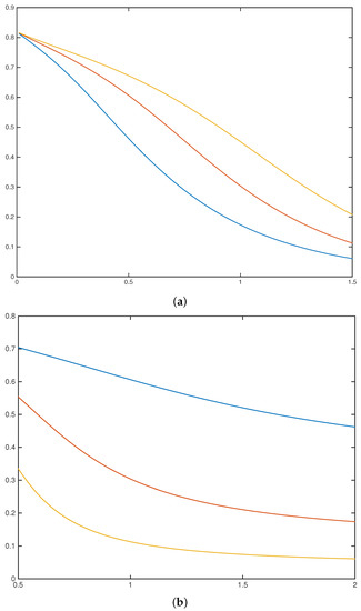
Figure 3. The option price ${\varphi }_0\left(x\right),x=2,$ in the case $c_0=1, c_1=0.5,r=0.1:$ (a): versus the switching rate $\lambda ={\lambda }_0={\lambda }_1,$ $\lambda \le 1.5,$ for the different values $b_0=b_1=b=0.5/1.0/1.5$ (from bottom to top); (b): versus the mean jump amplitude, $m=b^{-1},b=b_0=b_1,$ $0.5\le m\le 2,$ for different switching rates ${\lambda }_0={\lambda }_1=\lambda =0.5/1.0/1.5$ (from top to bottom).

Consider another simplified case where there are explicit formulae.

Example 2.

Let jump amplitudes be distributed with (20), and ${\beta }_0=b_0$ and ${\beta }_1=b_1$. In this case, Equation (18) becomes

$$({\alpha }^2-b_0^2)({\alpha }^2-b_1^2)=a^2,a^2=\frac{{\lambda }_0{\lambda }_1{b}_0{b}_1}{c_0{c}_1}.$$

(26)

If$b_0^2{b}_1^2>a^2,$then Equation (26) has exactly two real positive roots ${\alpha }_0$ and ${\alpha }_1,$ and two real negative, $-{\alpha }_0,-{\alpha }_1,$

$$0<{\alpha }_0<b_0^2\wedge b_1^2,{\alpha }_1>b_0^2\vee b_1^2,$$

$${\alpha }_0=\sqrt{\frac{b_0^2+b_1^2-\sqrt{{(b_0^2-b_1^2)}^2+4a^2}}{2}},{\alpha }_1=\sqrt{\frac{b_0^2+b_1^2+\sqrt{{(b_0^2-b_1^2)}^2+4a^2}}{2}}.$$

In this case, the solution is obtained by (14) with coefficients given by (19).

In the case$b_0^2{b}_1^2<a^2,$the Equation (18) has only one positive real root ${\alpha }_1$ (and one negative one $-{\alpha }_1;$ there are also a couple of conjugate imaginary roots). The solution is ${\varphi }_0\left(x\right)={\varphi }_1\left(x\right)={\mathrm{e}}^{-{\alpha }_{1}x}$.

3.2. “Bull Market” and Negative Threshold

A process with positive trends $c_0>c_1>0$ breaches the threshold $x<0$ only by jumping. It cannot pass this level without switching, and the problem becomes much more difficult. Similarly to Section 3.1, we obtain the integral equations

$$\begin{array}{cc}\hfill {\varphi }_0\left(x\right)=& {\int }_0^{\infty }{\lambda }_0{\mathrm{e}}^{-(r+{\lambda }_0)t}{H}_0(x-c_{0}t)\mathrm{d}t+{\int }_0^{\infty }{\lambda }_0{\mathrm{e}}^{-(r+{\lambda }_0)t}\mathrm{d}t\underset{-1+exp(x-c_{0}t)}{\overset{0}{\int }}{\varphi }_1(x-c_{0}t-log(1+y))h_0\left(\mathrm{d}y\right),\hfill \end{array}$$

(27)

$$\begin{array}{cc}\hfill {\varphi }_1\left(x\right)=& {\int }_0^{\infty }{\lambda }_1{\mathrm{e}}^{-(r+{\lambda }_1)t}{H}_1(x-c_{1}t)\mathrm{d}t+{\int }_0^{\infty }{\lambda }_1{\mathrm{e}}^{-(r+{\lambda }_1)t}\mathrm{d}t\underset{-1+exp(x-c_{1}t)}{\overset{0}{\int }}{\varphi }_0(x-c_{1}t-log(1+y))h_1\left(\mathrm{d}y\right),\hfill \end{array}$$

(28)

where the cumulative distribution function

$$H_i\left(x\right)=\mathbb{P}\{log(1+Y)<x|ϵ\left(0\right)=i\}=\mathbb{P}\{Y<-1+{\mathrm{e}}^x|ϵ\left(0\right)=i\},i\in \{0,1\},$$

$b_0,b_1>0,$ corresponds to the jump occurring in state i. The first terms of these equations appear under the condition of breakdown of the threshold after the first jump, the second terms correspond a small jump, not enough to immediately exercise the option.

In the case of exponentially distributed log-jumps, Equations (27) and (28) become slightly simpler. Indeed, let (negative) jumps have alternating distributions with the accumulated distribution function

$$H_i\left(x\right)={\mathbb{P}}_i\{log(1+Y)<x\}={\mathrm{e}}^{b_{i}x}\wedge 1,i\in \{0,1\},$$

see (20).

Note that

$${\int }_0^{\infty }\lambda {\mathrm{e}}^{-(r+\lambda )t}{H}_0(x-ct)\mathrm{d}t={\int }_{x/c}^{\infty }\lambda {\mathrm{e}}^{-(r+\lambda )t}{\mathrm{e}}^{b(x-ct)}\mathrm{d}t=\frac{\lambda {\mathrm{e}}^{-(r+\lambda )x/c}}{r+\lambda +bc},$$

and changing the order of integration, we obtain

$$\begin{array}{l}{\int }_0^{\infty }\lambda {\mathrm{e}}^{-(r+\lambda )t}\mathrm{d}t{\int }_{x-ct}^0\varphi (x-ct-log(1+y))b{(1+y)}^{b-1}\mathrm{d}y\\ ={\int }_{-\infty }^0\varphi \left(z\right)b{\mathrm{e}}^{b(x-z)}\mathrm{d}z{\int }_{\frac{x-z}{c}\wedge 0}^{\infty }\lambda {\mathrm{e}}^{-(r+\lambda +bc)t}\mathrm{d}t\\ =\frac{b\lambda }{r+\lambda +bc}\left. [{\int }_x^0\varphi \left(z\right){\mathrm{e}}^{b(x-z)}\mathrm{d}z+{\int }_{-\infty }^x\varphi \left(z\right){\mathrm{e}}^{-(r+\lambda )(x-z)/c}\mathrm{d}z\right]\end{array}$$

Therefore, Equations (27) and (28) take the form

$$\begin{array}{cc}\hfill {\varphi }_0\left(x\right)& =\frac{{\lambda }_0}{r+{\lambda }_0+b_0{c}_0}\left. [{\mathrm{e}}^{b_{0}x}+b_0{\int }_x^0{\mathrm{e}}^{b_0(x-z)}{\varphi }_1\left(z\right)\mathrm{d}z+b_0{\int }_{-\infty }^x{\mathrm{e}}^{-(r+{\lambda }_0)(x-z)/c_0}{\varphi }_1\left(z\right)\mathrm{d}z\right],\hfill \\ \hfill {\varphi }_1\left(x\right)& =\frac{{\lambda }_1}{r+{\lambda }_1+b_1{c}_1}\left. [{\mathrm{e}}^{b_{1}x}+b_1{\int }_x^0{\mathrm{e}}^{b_1(x-z)}{\varphi }_0\left(z\right)\mathrm{d}z+b_1{\int }_{-\infty }^x{\mathrm{e}}^{-(r+{\lambda }_1)(x-z)/c_1}{\varphi }_0\left(z\right)\mathrm{d}z\right].\hfill \end{array}$$

(29)

With additional symmetry assumptions ${\lambda }_0={\lambda }_1=\lambda ,c_0=c_1=c$, and $b_0=b_1=b,$ these equations give the ruin probability. In this symmetric case, we have ${\varphi }_0={\varphi }_1=\varphi ,$ and, under the net profit condition $bc>\lambda ,$ the ruin probability $\mathbb{P}\left\{\mathcal{T}\right(x)<\infty \}$ is given explicitly:

$${\mathbb{P}\{\mathcal{T}\left(x\right)<\infty \}=\varphi \left(x\right)|}_{r=0}={\displaystyle \frac{\lambda }{bc}}exp\left(x(b-\lambda /c)\right),$$

which can be proved by plugging this expression into coinciding Equation (29). This repeats the known results, see, e.g., [12] (5.3.8).

3.3. “Bear Market” and the Cram ér–Lundberg Ruin Model

Let both trends be negative, $0>c_0>c_1,x<0,$ and jumps positive. This case is symmetric to bullish market with negative corrections described in Section 3.1. In this case, the Laplace transform $\overrightarrow{\varphi }$ of $\mathcal{T}\left(x\right)$ is given by Formula (14) with the negative exponential rates ${\alpha }_1,{\alpha }_2$ given by the Equation (18).

4. Appendix: How to Choose a Martingale Measure

Since Equation (6) can has infinite number of solutions ${\phi }_0,{\phi }_1,$ this model typically has infinitely many risk-neutral measures. In order to choose an appropriate martingale measure, we presume some additional restrictions.

• Jump risk is not priced. Note that the telegraph process $X=X\left(t\right)$ and the accompanying Markov process ${ϵ}^{}$ can be considered as a source of systematic risk, while jump amplitudes can be classified as unsystematic. Under such assumptions, it is reasonable to assume that a change of the measure does not affect the distribution of jump amplitudes. This idea resembles the approach proposed by R.C.Merton [14].
  This corresponds to a constant solution of the Equation (6), which coincides with the new switching intensities, i.e., ${\phi }_0={\lambda }_0^{\ast }=(r_0-c_0)/y_0$ and ${\phi }_1={\lambda }_1^{\ast }=(r_1-c_1)/y_1$.
  To choose a risk-neutral measure, we apply the measure transformation determined by the Radon–Nikodym derivative,

  $$\frac{\mathrm{d}\tilde{\mathbb{P}}}{\mathrm{d}\mathbb{P}}={\mathcal{E}}_t(X^{\ast }+J^{\ast })=exp\left(X^{\ast }\left(t\right)\right){\kappa }_{N\left(t\right)}^{\ast },$$

  (30)

  where $X^{\ast }\left(t\right)=\underset{0}{\overset{t}{\int }}{c}_{{ϵ}^{(}u)}^{\ast }\mathrm{d}u,J^{\ast }\left(t\right)={\displaystyle \sum _{n=1}^{N\left(t\right)}}{y}_{{ϵ}^{(}{\tau }_n-)}^{\ast },{\kappa }_{N\left(t\right)}^{\ast }={\displaystyle \prod _{n=1}^{N\left(t\right)}}(1+y_{{ϵ}^{(}{\tau }_n-)}^{\ast })$ with deterministic constants $c_0^{\ast },c_1^{\ast }$ and $y_0^{\ast },y_1^{\ast }$ satisfying the martingale condition (5), i.e.,

  $$c_0^{\ast }+{\lambda }_0{y}_0^{\ast }=0,c_1^{\ast }+{\lambda }_1{y}_1^{\ast }=0.$$

  (31)
  For the measure $\tilde{\mathbb{P}}$ specified in this way, the distribution of jump amplitudes does not change, but the market regimes switch with changed rates ${\lambda }_0^{\ast },{\lambda }_1^{\ast },$ which are determined by

  $${\lambda }_0^{\ast }={\lambda }_0(1+y_0^{\ast })={\lambda }_0-c_0^{\ast },{\lambda }_1^{\ast }={\lambda }_1(1+y_1^{\ast })={\lambda }_1-c_1^{\ast }.$$

  (32)
  By virtue of (31), it is clear that transformation (30) leads to a risk-neutral measure $\tilde{\mathbb{P}}$ for this market model if and only if

  $$c_i^{\ast }={\lambda }_i+c_i/y_i\mathrm{and}{y}_i^{\ast }=-c_i^{\ast }/{\lambda }_i=-1-c_i/\left({\lambda }_i{y}_i\right),i\in \{0,1\}.$$
  With this martingale measure, the switching rates ${\lambda }_0^{\ast }$ and ${\lambda }_1^{\ast }$ are given by

  $${\lambda }_0^{\ast }=-\frac{c_0}{y_0},{\lambda }_1^{\ast }=-\frac{c_1}{y_1}.$$

  (33)
  See [3,5] for details.
• Jump risk is insured. To choose another risk-neutral measure, we supply the market with an additional security, which magnifies its value by a fixed rate every time there is a change of the market state, i.e., let

  $$\widehat{S}\left(t\right)=\prod _{n=1}^{N\left(t\right)}(1+{\widehat{y}}_n)$$

  (34)
  Here, the process $\widehat{S}\left(t\right)$ is governed by the same Poisson process $N,$ and it has deterministic jump values ${\widehat{y}}_n,{\widehat{y}}_n>0$. This security can be considered as insurance that compensates losses and gains provoked by state changes and helps to hedge the option with a general payoff function $\mathcal{H}=f(S,\widehat{S})$. A market formed by three assets $B,S,\widehat{S}$ is still incomplete, but now we can use the following approach to make a reasonable choice of risk-neutral measure. First, we change the measure with respect to the switching intensities. Assume the magnification coefficients ${\widehat{y}}_n$ alter according to alternating market states, ${\widehat{y}}_n\in \{{\widehat{y}}^{\left(0\right)},{\widehat{y}}^{\left(1\right)}\}.$ Applying the Radon–Nikodym derivative (30) to the asset $\widehat{S},$ we define the equivalent measure with switching intensities ${\lambda }_i^{\ast }=r_i/{\widehat{y}}^{\left(i\right)}$. We then make one more change of measure, conserving the form of the distribution of the jump values $Y_n$.

The following example illustrates this approach.

Example 3.

(Log-exponential distribution). Let jumps $Y_n$ be distributed with the alternating probability density functions $h_i\left(\mathrm{d}y\right)=b_i{(1+y)}^{-1+b_i}{\mathrm{𝟙}}_{\{-1<y<0\}}\mathrm{d}y,i\in \{0,1\},$ where $b_0,b_1>0,$ see (20), which is equivalent to the negative exponential distribution of $log(1+Y_n)$ with the probability density function $b_{i}exp\left(b_{i}x\right){\mathrm{𝟙}}_{\{x<0\}}$.

Consider a measure transformation that preserves the form of the jump distribution, which is defined by a solution to (6) of the form ${\phi }_i\left(x\right)={\delta }_i{(1+y)}^{d_i}{\mathrm{𝟙}}_{\{-1<y<0\}},i\in \{0,1\}$. By virtue of (6), the positive parameters ${\delta }_i$ and $d_i$ satisfy the equation

$$-r_i+c_i+\frac{b_i{\delta }_i}{(b_i+d_i)(1+b_i+d_i)}=0.$$

Since by virtue of (7), we have

$${\lambda }_i^{\ast }=b_i{\delta }_i{\int }_{-1}^0{(1+y)}^{-1+b_i+d_i}\mathrm{d}y=\frac{b_i{\delta }_i}{b_i+d_i},$$

therefore,

$$d_i=-1-b_i+\frac{{\lambda }_i^{\ast }}{c_i-r_i}\mathit{and}{\delta }_i=\frac{{\lambda }_i^{\ast }}{b_i}\left(-1+\frac{{\lambda }_i^{\ast }}{c_i-r_i}\right),$$

(35)

where the new switching intensities ${\lambda }_i^{\ast }$ are determined at the first step: ${\lambda }_i^{\ast }=r_i/{\widehat{y}}^{\left(i\right)}$.

Since$d_i>0,$we have the condition for the insurance coefficients${\widehat{y}}^{\left(i\right)}:$

$$0<{\widehat{y}}^{\left(i\right)}<r_i{(c_i-r_i)}^{-1}{(1+b_i)}^{-1},$$

which is sufficient for the existence of a risk-neutral measure.

The new distributions of jump amplitudes are

$$h_i^{\ast }\left(\mathrm{d}y\right)=(b_i+d_i){(1+y)}^{-1+b_i+d_i}\mathrm{d}y·{\mathrm{𝟙}}_{\{-1<y<0\}},i\in \{0,1\}.$$

References

- Goldstein, S. On diffusion by discontinuous movements and on the telegraph equation. Q. J. Mech. Appl. Math. 1951, 4, 129–156. [Google Scholar] [CrossRef]
- Kac, M. A stochastic model related to the telegrapher’s equation. Rocky Mt. J. Math. 1974, 4, 497–509, reprinted in Kac, M. Some Stochastic Problems in Physics and Mathematics; Colloquium lectures in the pure and applied sciences, No. 2, hectographed; Field Research Laboratory, Socony Mobil Oil Company: Dallas, TX, USA, 1956; pp. 102–122.. [Google Scholar] [CrossRef]
- Ratanov, N. A jump telegraph model for option pricing. Quant. Financ. 2007, 7, 575–583. [Google Scholar] [CrossRef]
- López, O.; Ratanov, N. Option pricing driven by a telegraph process with random jumps. J. Appl. Probab. 2012, 49, 838–849. [Google Scholar] [CrossRef]
- Ratanov, N.; Kolesnik, A.D. Telegraph Processes and Option Pricing, 2nd ed.; Springer: Heidelberg, Germany; New York, NY, USA; Dordrecht, The Netherlands; London, UK, 2022. [Google Scholar]
- Ratanov, N. Telegraph Processes and Option Pricing; 2nd Nordic-Russian Symposium on Stochastic Analysis; Springer: Beitostolen, Norway, 1999. [Google Scholar]
- Di Crescenzo, A.; Pellerey, F. On prices’ evolutions based on geometric telegrapher’s process. Appl. Stoch. Model. Bus. Ind. 2002, 18, 171–184. [Google Scholar] [CrossRef]
- Dalang, R.C.; Hongler, M.-O. The right time to sell a stock whose price is driven by Markovian noise. Ann. Appl. Probab. 2004, 14, 2176–2201. [Google Scholar] [CrossRef]
- Jeanblanc, M.; Yor, M.; Chesney, M. Mathematical Methods for Financial Markets; Springer: Dordrecht, The Netherlands; Heidelberg, Germany; London, UK; New York, NY, USA, 2009. [Google Scholar]
- Rubinstein, M.; Reiner, E. Unscrambling the binary code. Risk Mag. 1991, 4, 75–83. [Google Scholar]
- Linz, P. Analytical and Numerical Methods for Volterra Equations; SIAM: Philadelphia, PN, USA, 1985. [Google Scholar]
- Rolski, T.; Schmidli, H.; Schmidt, V.; Teugels, J. Stochastic Processes for Insurance and Finance; John Wiley & Sons: Hoboken, NJ, USA, 1999. [Google Scholar]
- Prudnikov, A.P.; Brychkov, Y.A.; Marichev, O.I. Integrals and Series, Vol. 5. Inverse Laplace Transforms; Gordon and Breach Science Publishers: Langhorne, PA, USA, 1992. [Google Scholar]
- Merton, R.C. Option pricing when underlying stock returns are discontinuous. J. Financ. Econom. 1976, 3, 125–144. [Google Scholar] [CrossRef]
Publisher’s Note: MDPI stays neutral with regard to jurisdictional claims in published maps and institutional affiliations. |
© 2022 by the author. Licensee MDPI, Basel, Switzerland. This article is an open access article distributed under the terms and conditions of the Creative Commons Attribution (CC BY) license (https://creativecommons.org/licenses/by/4.0/).