Cayley Hash Values of Brauer Messages and Some of Their Applications in the Solutions of Systems of Differential Equations

Abstract

Cayley hash values are defined by paths of some oriented graphs (quivers) called Cayley graphs, whose vertices and arrows are given by elements of a group $\mathfrak{H}$. On the other hand, Brauer messages are obtained by concatenating words associated with multisets constituting some configurations called Brauer configurations. These configurations define some oriented graphs named Brauer quivers which induce a particular class of bound quiver algebras named Brauer configuration algebras. Elements of multisets in Brauer configurations can be seen as letters of the Brauer messages. This paper proves that each point $(x,y)\in \mathcal{V}=\mathbb{R}\backslash \left\{0\right\}\times \mathbb{R}\backslash \left\{0\right\}$ has an associated Brauer configuration algebra ${\Lambda }_{{\mathfrak{B}}^{(x,y)}}$ induced by a Brauer configuration ${\mathfrak{B}}^{(x,y)}$. Additionally, the Brauer configuration algebras associated with points in a subset of the form $(\lfloor (x)\rfloor ,\lceil (x)\rceil ]\times (\lfloor (y)\rfloor ,\lceil (y)\rceil ]\subset \mathcal{V}$ have the same dimension. We give an analysis of Cayley hash values associated with Brauer messages $\mathfrak{M}\left({\mathfrak{B}}^{(x,y)}\right)$ defined by a semigroup generated by some appropriated matrices $A_0,A_1,A_2\in \mathrm{GL}(2,\mathcal{R})$ over a commutative ring $\mathcal{R}$. As an application, we use Brauer messages $\mathfrak{M}\left({\mathfrak{B}}^{(x,y)}\right)$ to construct explicit solutions for systems of linear and nonlinear differential equations of the form $X^{″}\left(t\right)+MX\left(t\right)=0$ and $X^{\prime }\left(t\right)-X^2\left(t\right)N\left(t\right)=N\left(t\right)$ for some suitable square matrices, M and $N\left(t\right)$. Python routines to compute Cayley hash values of Brauer messages are also included.

1. Introduction

Hash functions are compression functions that are easy to compute. They are helpful tools in several cryptographic tasks. Ensuring data integrity and password authentication systems are some of the primary roles of hash functions. Data integrity provided by hash functions prevents undesirable data modification [1].

To date, it is believed that well-posed hash functions such as SHA256 are unbreakable by several attacks, including those conducted by a quantum computer.

The Cayley graph ${\mathcal{C}}_{\mathfrak{H},\mathfrak{s}}=(V,E)$ associated with a subset $\mathfrak{s}$ of a multiplicative (semi)group $\mathfrak{H}$ is a k-regular graph, whose set of vertices V are in bijective correspondence with the set $\mathfrak{H}$. In this case, if $v_{g_1},v_{g_2}\in V$ are vertices corresponding to the elements $g_1,g_2\in \mathfrak{H}$, then there is an arrow connecting $v_{g_1}$ and $v_{g_2}$ provided that there is an element $s\in \mathfrak{s}$, such that $g_1^{-1}{g}_2{s}^{-1}=1$, where 1 is the identity element of the group $\mathfrak{H}$. The idea behind the use of Cayley graphs in cryptography is to produce hash functions that are collision resistant. The input to these functions gives directions for walking around the graph, and the output is the ending vertex of the walk [2].

On the other hand, Brauer messages were introduced by Espinosa et al. [3] in their research regarding some bound quiver algebras called Brauer configuration algebras by Green and Schroll [4]. This paper provides Cayley hash values to some of these Brauer messages.

Brauer messages have applications in different science fields. For instance, they were used by Cañadas et al. in the graph energy theory to compute the trace norm of some matrices and in the war games theory to declare winners and losers in war games based on the behavior of a missile defense system (MDS) [5]. Furthermore, mutations of Brauer messages can be used to give an algebraic interpretation of the Advanced Encryption Standard (AES) key schedule [6].

1.1. Motivations

This paper uses an interaction between cryptography, algebraic geometry, combinatorics, and the theory of representation of associative algebras to obtain applications of the theory of Brauer configuration algebras in cryptography and differential equations.

Relationships between algebraic geometry and Brauer configuration algebras are motivated by a recent paper published by Green and Schroll [7], who proved that each point in an affine variety has an associated suitable associative algebra and that all these algebras have the same dimension. As an interpretation of this result, we prove that, associated with each point in ${\mathbb{R}}^{*}\times {\mathbb{R}}^{*}$, there is a suitable Brauer configuration algebra and that Brauer configuration algebras associated with points in a set of the form $(m,m+1]\times (n,n+1],m,n\in \mathbb{Z}$ have the same dimension. The messages arising from these Brauer configurations (called Brauer messages) are used to provide solutions for linear and nonlinear systems of differential equations. We compute Cayley hash values of Brauer messages establishing for which integer numbers such hash values are collision-resistant.

Henceforth, we outline the main results presented in this paper and how previous works are used to obtain them.

1.2. Contributions

We prove that each point $(x,y)\in \mathcal{V}=\mathbb{R}\backslash \left\{0\right\}\times \mathbb{R}\backslash \left\{0\right\}$ is associated with a suitable Brauer configuration algebra. Properties of these algebras are also established. In particular, it is proved that their dimensions can be computed by enumerating suitable lattice paths. Similar conditions have their corresponding centers.

As an application, we interpret message specializations of these Brauer configurations as appropriated matrices with applications in Catalan combinatorics and differential equations. It is also proved that some of these matrices are solutions to some linear and nonlinear systems of differential equations of the form $X^{″}\left(t\right)+2^{\gamma -1}X\left(t\right)=0$ and  $X^{\prime }\left(t\right)-X^2\left(t\right){\mathfrak{M}}^{\mathfrak{e}}(\alpha ,\gamma ,\beta )t={\mathfrak{M}}^{\mathfrak{e}}(\alpha ,\gamma ,\beta )t$, where ${\mathfrak{M}}^{\mathfrak{e}}(\alpha ,\gamma ,\beta$) is a matrix whose entries are given by appropriated Brauer messages. It is worth noting that finding explicit solutions to nonlinear differential equations is in general a cumbersome problem.

Cayley hash functions based on matrix semigroups are applied to some Brauer messages to prove that these hash families are collision resistant.

Python routines to compute Cayley hash values of Brauer messages associated with points in the plane are also introduced.

Figure 1 shows how previous works, mutations, and Brauer configuration algebras (BCAs) can be related to obtain the main results (targets of red arrows) presented in this paper.

In Section 2.1.1, we recall the main results regarding BCAs; Proposition 1 and Theorem 2 give formulas for the dimensions of these algebras and their centers.

Theorem 3 provides the properties of BCAs associated with points in the plane. Their dimensions and combinatorial data regarding indecomposable projective modules over these algebras are given.

Theorem 4 describes arithmetic properties of specialized matrices given by mutations of Brauer configurations associated with the plane.

Corollary 1 provides explicit solutions of linear and nonlinear systems of differential equations.

Section 4 is devoted to Cayley hash functions. Theorem 5 gives Cayley hash values for appropriated matrix semigroups. These results allow to give Cayley hash values of Brauer messages. Corollary 2 proves that Sosnovski hash functions are collision-resistant when they are applied to Brauer messages.

This paper is distributed as follows: Section 2 is devoted to recalling definitions and notation used throughout the document. In particular, we recall the notion of Brauer configuration algebra. In Section 3, we give our main results. We associate to each point $(x,y)\in \mathcal{V}$ an apropriated Brauer configuration algebra determining which of them have the same dimension. Mutations are defined for the variables associated with these algebras. Such mutations give rise to new classes of matrices with applications in combinatorics and differential equations. Section 4 is devoted to the values of Cayley hash functions associated with Brauer messages. Experimental data are given in Section 5. Concluding remarks and possible future works are described in Section 6. Appendix A gives Python routines to compute Brauer messsages, their Sosnovski hash values, and polygons of Brauer configurations associated with the plane.

2. Background and Related Work

In this section, we introduce some definitions and notation to be used throughout the paper. In particular, a brief overview regarding hash functions and Brauer configuration algebras is given [4].

Henceforth, the symbol $\mathbb{F}$ ($\mathbb{C})$ denotes a field (the complex numbers field), and $\lceil \left(x\right)\rceil$ ($\lfloor \left(x\right)\rfloor$) denotes the smallest (greatest) integer greater (less) than or equal to a real number x. In path algebras $\mathbb{F}Q$, it is assumed that $\mathbb{F}$ is an algebraic closed field.

2.1. Related Work on Cayley Hash Functions

This section gives a background on hash functions, in particular, Cayley hash functions.

Hash functions are easy-to-compute compression functions, as described before. Such functions are used in several contexts. For instance, they are helpful in password management systems. Servers that authenticate user passwords save a one-way hash associated with a unique password so that if an attacker steals the database, it may be unfeasible for the attacker to recover the original password as plaintext [1,8].

A hash family is a four-tuple $(\mathcal{X},\mathcal{Y},\mathcal{K},\mathcal{H})$, where

• $\mathcal{X}$ is a set of possible messages, which could be finite or infinite.
• $\mathcal{Y}$ is a finite set of possible message digests or authentication tags.
• $\mathcal{K}$ is the set of keys.
• For each $k\in \mathcal{K}$, there is a hash function $h_K:\mathcal{X}\to \mathcal{Y}\in \mathcal{H}$. If $\left|\mathcal{X}\right|$ and $\left|\mathcal{Y}\right|$ denote the cardinals of $\mathcal{X}$ and $\mathcal{Y}$, and $2\left|\mathcal{Y}\right|\le \left|\mathcal{X}\right|$, then $h_k$ is said to be a compression function. If $\mathcal{X}=\mathcal{Y}$, and the hash function h is the identity, then h is said to be an unkeyed hash function [1,2].

A hash function is said to be secure if the following three problems are difficult to solve:

Preimage 

Instance: A hash function $h:\mathcal{X}\to \mathcal{Y}$ and an element $y\in \mathcal{Y}$.

Find: $x\in \mathcal{X}$ such that $h\left(x\right)=y$. 

Second Preimage 

Instance: A hash function $h:\mathcal{X}\to \mathcal{Y}$ and an element $x\in \mathcal{X}$.

Find: $x^{\prime }\in \mathcal{X}$ such that $x^{\prime }\ne x$ and $h\left(x^{\prime }\right)=h\left(x\right)$. 

Collision

Instance: A hash function $h:\mathcal{X}\to \mathcal{Y}$ and an element $x\in \mathcal{X}$.

Find: $x,x^{\prime }\in \mathcal{X}$ such that $x^{\prime }\ne x$ and $h\left(x^{\prime }\right)=h\left(x\right)$.  

Hash functions are used to construct a short fingerprint or digest the message of some data. If an attacker alters the data, then the fingerprint will no longer be valid. One of the most used methods to construct iterated hash functions is the Merkle–Damgård scheme, which builds hash functions from a compression function. Rivest introduced, in 1990, the first scheme of this type named MD4. Soon afterwads, Rivest himself proposed an improved version of MD4 called MD5.

Collisions in the compression function of MD4 and MD5 were discovered in the 1990s.

The family of secured hash algorithms (SHAs) was proposed as a standard by NIST in 1993. SHA-0 was adopted as FIPS 180. Each of these hash algorithms was an improvement of the earlier versions to prevent previously found attacks.

It was shown in 1998 that SHA-0 allows collisions in approximately $2^{61}$ steps, whereas the first collision for SHA-1 was found in 2017. SHA-2 includes the four hash functions known as SHA-224, SHA-256, SHA-384, and SHA-512, according to the sizes of the corresponding fingerprints. It is worth pointing out that currently SHA-256, which outputs 256 bits fingerprints, is the most used hash function. It is the basis of many password authentication systems.

According to the National Academy of Sciences, Engineering, and Medicine [8] (NAE), although, nowadays it is believed to be essentially impossible to break a hash function such as SHA-256, password hashing is at higher risk due to the size of all 10-character passwords being only about $2^{66}$ passwords, and thus prone to an attack based on a quantum computer.

Possible attacks on the currently used hash functions have encouraged the use of provably secure hash functions, whose security is based on the difficulty of solving a known hard problem.

Cayley hash functions based on the Cayley graph of certain (semi)groups are examples of these types of schemes, whose security follows from the hardness of the expander graph problem associated with a (semi)group.

In 1991, Zémor [9] introduced hash function schemes based on matrix products in the special linear group $\mathrm{Sl}\left({\mathbb{F}}_p\right)$, where p is a fixed prime number. Zémor himself and Tillich [10] broke such schemes. Furthermore, they introduced the group $\mathrm{Sl}\left({\mathbb{F}}_{2^n}\right)$ to increase the security of the original hash functions [11]. In this setting, ${\mathbb{F}}_{2^n}$ is a field.

Due to the popularity of the hash functions introduced by Zémor and Tillich, several proposals in the same line were proposed by Petit and Lubotzki et al., who introduced Cayley hash functions based on Ramanujan graphs, in particular LPS hash functions [12,13,14,15].

The Tillich–Zémor hash function hashes each bit of a given message individually. In this case, the matrices have the form $A=\left[\begin{array}{cc}\alpha & 1\\ 1& 0\end{array}\right]$ and $B=\left[\begin{array}{cc}\alpha & \alpha +1\\ 1& 1\end{array}\right]$, where ${\mathbb{F}}_{2^n}=F_2\left[x\right]/\left(p\left(x\right)\right)$, $F_2$ is the two-element field, $\left(p\right(x\left)\right)$ is the ideal generated by an irreducible polynomial of degree n, and $\alpha$ is a root of $p\left(x\right)$. For instance, the message $M=110011$ is hashed to the matrix $B^2{A}^2{B}^2$.

It is worth noting that the Tillich–Zémor hash function was successfully attacked by Grass et al. [16], who obtained collisions using the Euclidean algorithm for polynomials. Afterwards, Petit and Quisquater [17] introduced an extended form of Grass et al.’s algorithm to provide a second preimage algorithm. Grassl et al. also ran Grover’s algorithm on a quantum computer to study the strength of the cryptographic system AES [18].

Mullan and Tsaban [19] introduced a general attack for the Tillich–Zémor scheme. It runs with polynomial time $o\left(\sqrt{q}\right)$ to find collisions for an arbitrary q. It does not work for bit strings of length $n>100$.

Other pairs of matrices such as in the Tillich–Zémor scheme have been proposed by Bromber et al. and Sosnovki, who introduced a semigroup platform corresponding to the hash functions $f\left(x\right)=2x+1$ and $g\left(x\right)=3x+1$ modulo a prime $p>3$ (the corresponding associated matrices have the form $A=\left[\begin{array}{cc}2& 1\\ 0& 1\end{array}\right]$ and $B=\left[\begin{array}{cc}3& 1\\ 0& 1\end{array}\right]$). In this case, the input string hash function can have an arbitrary length, and the output has the size $2log\left(p\right)$.

In this paper, we applied Sosnovski hash functions to Brauer messages to investigate their collision-resistant property.

2.1.1. Background and Related Work on Brauer Configuration Algebras

Brauer configuration algebras (BCAs) were introduced by Green and Schroll [4] to generalize research on tame algebras. Soon afterwards, Cañadas et al. used these algebras and their associated messages to obtain applications in cryptography, cibersecurity, and the graph energy theory [3,5,6,20,21].

It is worth pointing out that Espinosa [3] introduced in his doctoral dissertation the notion of the message of a Brauer configuration as the element of a word algebra. He used Brauer messages to give formulas for the number of perfect matchings of a snake graph and the number of homological ideals associated with a Nakayama algebra. On the other hand, Cañadas et al. introduced mutations of Brauer configurations to give an algebraic description of the cryptosystem AES [6].

In this paper, we associate Brauer configuration algebras with points in the plane, establishing which points have associated Brauer configuration algebras with the same dimension.

2.1.2. Path Algebras

In this section, we give a brief discussion on quivers, path algebras, and their ideals based on the work of Assem et al. [22].

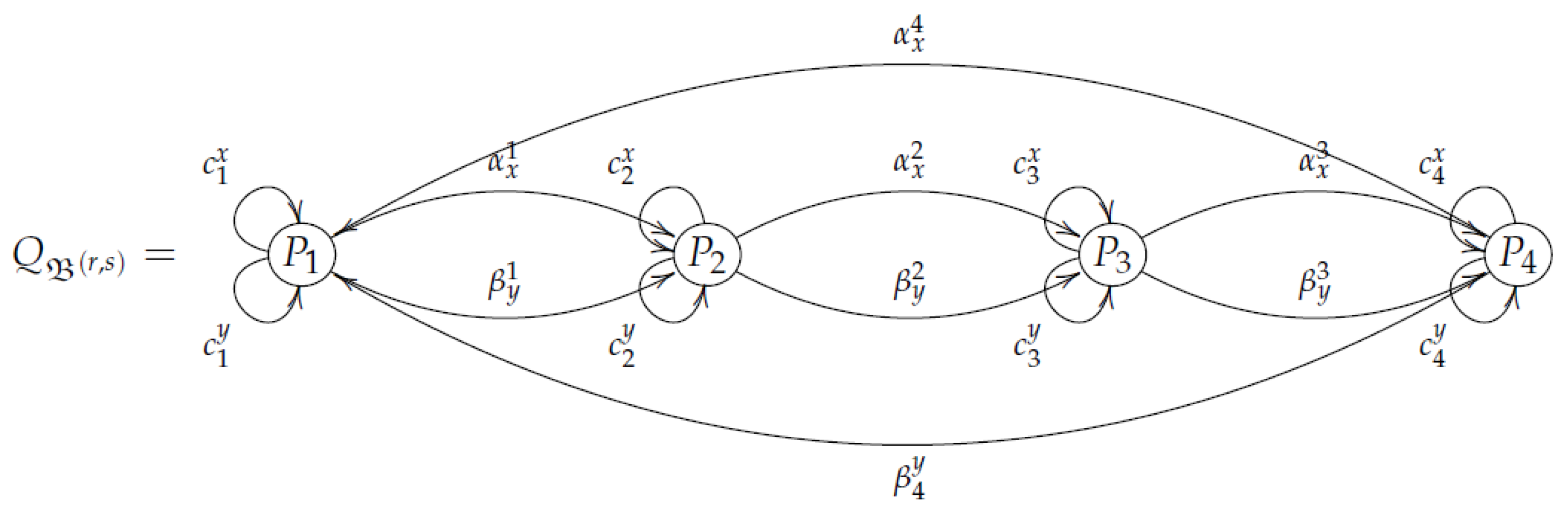
A quiver or directed graph $Q=(Q_0,Q_1)$ is a quadruple consisting of two sets: $Q_0$ (whose elements are called points or vertices) and $Q_1$ (whose elements are called arrows) and two maps $s,t:Q_1\to Q_0$ which associate to each arrow $\alpha \in Q_1$, its source $s\left(\alpha \right)\in Q_0$, and its target $t\left(\alpha \right)\in Q_0$, respectively. If $\mathbb{F}$ is an algebraically closed field, then we let $\mathbb{F}Q$ denote the path algebra associated with the quiver Q, whose underlying $\mathbb{F}$-vector space has as its basis the set of all paths of length $l\ge 0$ in Q,  such that the product of two basis vectors is given by the usual concatenation of paths.

The following Figure 2 shows a quiver Q with four vertices $a_1,a_2$, $a_3$, and $a_4$ and three arrows ${\alpha }_1$, ${\alpha }_2$, and ${\alpha }_3$. Note that, $Q_1=\{{\alpha }_1,{\alpha }_2,{\alpha }_3\}$ is the set of paths of length 1, whereas $Q_2=\{{\alpha }_1{\alpha }_2,{\alpha }_1{\alpha }_3\}$ is the set of paths of length 2 in Q.

The basis $\mathcal{B}$ of the algebra $\mathbb{F}Q$ associated with the quiver Q shown in Figure 2 is $\mathcal{B}=\{e_{a_1},e_{a_2},e_{a_3},e_{a_4},{\alpha }_1,{\alpha }_2,{\alpha }_3,{\alpha }_1{\alpha }_2,{\alpha }_1{\alpha }_3\}$, where $\{e_{a_1},e_{a_2},e_{a_3},e_{a_4}\}$ is the set of primitive idempotents, with $e_{a_i}^2=e_{a_i}$ and $e_{a_i}{e}_{a_j}=0$ if $i\ne j$.

Let Q be a finite and connected quiver. The two-sided ideal$R_Q$ of the path algebra $\mathbb{F}Q$ generated (as an ideal) by the arrows of Q is called the arrow ideal of $\mathbb{F}Q$. A two-sided ideal I of $\mathbb{F}Q$ is said to be admissible if there exists $m\ge 2$ such that $R_Q^m\subseteq I\subseteq R_Q^2$.

If I is an admissible ideal of $\mathbb{F}Q$, the pair $(Q,I)$ is said to be a bound quiver. The quotient algebra $\mathbb{F}Q/I$ is said to be the algebra of the bound quiver $(Q,I)$ or, simply, a bound quiver algebra.

Let Q be a quiver. A relation in Q with coefficients in $\mathbb{F}$ is an $\mathbb{F}$-linear combination of paths of length, with at least two having the same source and target.

If ${\left({\rho }_j\right)}_{j\in J}$ is a set of relations for a quiver Q such that the ideal they generate $\langle {\rho }_j\mid j\in J\rangle$ is admissible, we say that the quiver Q is bound by the relation ${\left({\rho }_j\right)}_{j\in J}$ or by the relations ${\rho }_j=0$ [22].

Henceforth, we let $\mathrm{rad}\Lambda$ denote the radical of a path algebra $\Lambda =\mathbb{F}Q$, which is the intersection of all maximal ideals. Actually, if I is an admissible ideal of $\Lambda$, it holds that $\mathrm{rad}(\mathbb{F}Q/I)=R_Q/I$.

If ≺ is an admissible well-ordering on the set of paths, i.e.,  ≺ is a well-ordering such that

• If $a,b,u,v\in Q$, where $uav$ and $ubv$ are both nonzero $a\prec uav$ or $a=uav$.
• If $a\prec b$, then $uav\prec ubv$.

Then, the tip $Tip\left(x\right)=w$ of an element $x\in \mathbb{F}Q$ is the maximal path w with respect to ≺ such that w has a nonzero coefficient in x when it is written as a linear combination of the elements of a fixed basis of $\mathbb{F}Q$. $Tip\left(X\right)=\left\{Tip\right(x)\mid x\in X\}$ is the set of tips of elements in X [7].

Let I be an ideal in a path algebra $\mathbb{F}Q$ and let $\mathcal{G}\subset \mathcal{I}$. If $\langle Tip\left(\mathcal{G}\right)\rangle =\langle Tip\left(I\right)\rangle$, then $\mathcal{G}$ is a Gröbner basis for I with respect to ≺.

2.1.3. Brauer Configuration Algebras

In this section, we briefly discuss the main results regarding Brauer configuration algebras [4].

A Brauer configuration algebra ${\Lambda }_{\mathfrak{B}}$ (or simply $\Lambda$ if no confusion arises) is induced by a Brauer configuration $\mathfrak{B}=({\mathfrak{B}}_0,{\mathfrak{B}}_1,\mu ,\mathcal{O})$, consisting of a pair of finite sets ${\mathfrak{B}}_0$ and ${\mathfrak{B}}_1$, a function $\mu :{\mathfrak{B}}_0\to {\mathbb{N}}^{+}$ (${\mathbb{N}}^{+}$ denote the set of positive integers), and an orientation $\mathcal{O}$.

• Elements of ${\mathfrak{B}}_0$ (${\mathfrak{B}}_1$) are called vertices (polygons). Polygons are labeled multisets consisting of vertices.
• If $V\in {\mathfrak{B}}_1$, then $\left|V\right|>1$ (i.e., each polygon contains more than one vertex).
• $\mathcal{O}$ is a choice for each vertex $\delta \in {\mathfrak{B}}_0$ of a cyclic ordering of the polygons in which $\delta$ occurs as a vertex including repetitions (see [4] for more details). For instance, if a vertex $\delta \in {\mathfrak{B}}_0$ occurs in polygons $V_{i_i},V_{i_2},\cdots ,V_{i_m}$ for suitable indices, then the cyclic order is obtained by linearly ordering the list, say

  $$V_{i_1}^{{\mathfrak{d}}_1}<V_{i_2}^{{\mathfrak{d}}_2}<\cdots <V_{i_m}^{{\mathfrak{d}}_m},{\mathfrak{d}}_{i_s}>0,$$

  (1)

  where, $V_{i_s}^{{\mathfrak{d}}_s}=V_{i_s}^{\left(1\right)}<V_{i_s}^{\left(2\right)}<\cdots <V_{i_s}^{\left({\mathfrak{d}}_s\right)}$ means that vertex $\delta$ occurs ${\mathfrak{d}}_s$ times in polygon $V_{i_s}$, denoted ${\mathfrak{d}}_s=occ(\delta ,V_{i_s})$. The cyclic order is completed by adding the relation $V_{i_m}<V_{i_1}$. Note that if $V_{i_1}<\cdots <V_{i_t}$ is the chosen ordering at vertex $\delta$, then the same ordering can be represented by any cyclic permutation.
  The sequence (1) is said to be the successor sequence at vertex $\delta$, denoted $S_{\delta }$, which is unique up to permutations. Note that Green and Schroll [4] mentioned that different orientation choices are typically associated to nonisomorphic Brauer configuration algebras.
  Henceforth, in this paper, if a vertex ${\delta }^{\prime }\ne \delta$ belongs to some polygons $V_{j_1},V_{j_2},\cdots V_{j_k}$ ordered according to the already defined cyclic ordering associated with the vertex $\delta$, then we assume that up to permutations the cyclic ordering associated with the vertex ${\delta }^{\prime }$ is built, taking into account that polygons $V_{j_1},V_{j_2},\cdots V_{j_k}$ inherit the order given by the successor sequence $S_{\delta }$.
• If $\overline{V}$ denotes the underlying set defined by a polygon V (repetitions are not allowed in $\overline{V}$), then ${\displaystyle \bigcup _{V\in {\mathfrak{B}}_1}}\overline{V}={\mathfrak{B}}_0$.

If $\delta \in {\mathfrak{B}}_0$, then the valency $val\left(\delta \right)$ of $\delta$ is given by the identity

$$val\left(\delta \right)=\sum _{V\in {\mathfrak{B}}_1}occ(\delta ,V).$$

(2)

If $\delta \in {\mathfrak{B}}_0$ is such that $\mu \left(\delta \right)val\left(\delta \right)=1$, then $\delta$ is said to be truncated (it occurs once in just one polygon). Otherwise, $\delta$ is a nontruncated vertex. A Brauer configuration without truncated vertices is said to be reduced.

Algorithm 1 is a short version of an algorithm defined by Cañadas et al. in [5] to build a Brauer configuration algebra.

The following results describe the structure of Brauer configuration algebras [4,23].

Algorithm 1: Construction of a Brauer configuration algebra

Input A reduced Brauer configuration $\mathfrak{B}=({\mathfrak{B}}_0,{\mathfrak{B}}_1,\mu ,\mathcal{O})$. Output The Brauer configuration algebra ${\Lambda }_{\mathfrak{B}}=\mathbb{F}{Q}_{\mathfrak{B}}/I_{\mathfrak{B}}$. Construct the quiver $Q_{\mathfrak{B}}=({\left(Q_{\mathfrak{B}}\right)}_0,{\left(Q_{\mathfrak{B}}\right)}_1,s,t)$ as follows: ${\left(Q_{\mathfrak{B}}\right)}_0={\mathfrak{B}}_1$. For each covering $V_i<V_j$ in a successor sequence $S_{\delta }$, define an arrow $\stackrel{{\alpha }_i^{\delta }}{V_i\to V_j}\in {\left(Q_{\mathfrak{B}}\right)}_1$. For each path defined by a successor sequence $S_{\delta }$, construct a special cycle $C_{\delta }\in Q_{\mathfrak{B}}$ defined by the union $S_{\delta }\cup \{V_{i_m}<V_{i_1}\}$, where, $V_{i_1}=\min S_{\delta }$ and $V_{i_m}=\max S_{\delta }$. Define the path algebra $\mathbb{F}{Q}_{\mathfrak{B}}$. The admissible ideal $I_{\mathfrak{B}}$ is generated by relations of the following types: (a) Identify special cycles associated with nontruncated vertices in the same polygon (i.e., if ${\delta }_1,{\delta }_2\in U$ with $U\in {\mathfrak{B}}_1$, then $C_{{\delta }_1}^{\mu \left({\delta }_1\right)}\sim C_{{\delta }_2}^{\mu \left({\delta }_2\right)}$). (b) If $C_{\delta }$ is a special cycle associated with a nontruncated vertex $\delta$, then a product of the form $C^{\mu \left(\delta \right)}a\in I_{\mathfrak{B}}$ if a is the first arrow of $\delta$. (c) Products of the form $ab\in \mathbb{F}{Q}_{\mathfrak{B}}$ with a induced by a covering in a special cycle $C_{{\delta }_1}$ and b induced by another special cycle $C_{{\delta }_2}$ (with ${\delta }_1\ne {\delta }_2$) belong to $I_{\mathfrak{B}}$. ${\Lambda }_{\mathfrak{B}}=\mathbb{F}{Q}_{\mathfrak{B}}/I_{\mathfrak{B}}$ is a Brauer configuration algebra with a basis consisting of classes of special cycles and classes of prefixes of special cycles.

Theorem 1

([4], Theorem B, Proposition 2.7, Theorem 3.10, Corollary 3.12). Let ${\Lambda }_{\mathfrak{B}}$ be a Brauer configuration algebra with Brauer configuration $\mathfrak{B}=({\mathfrak{B}}_0,{\mathfrak{B}}_1,\mu ,\mathcal{O})$.

• There is a bijection between the set of indecomposable projective ${\Lambda }_{\mathfrak{B}}$-modules and the polygons of $\mathfrak{B}$. Moreover, if $P_V$ is an indecomposable ${\Lambda }_{\mathfrak{B}}$-module induced by a polygon V with r nontruncated vertices, then $\mathrm{rad}{P}_V={\displaystyle \underset{i=1}{\sum ^r}}{U}_i$, where for each i, $U_i$ is a uniserial ${\Lambda }_{\mathfrak{B}}$-module. $U_i\cap U_j$ is uniserial for all $1\le i,j\le r$.
• I is admissible, and  ${\Lambda }_{\mathfrak{B}}$ is multiserial and symmetric.
• The number of summands in the $\mathrm{rad}{P}_V/\mathrm{soc}{P}_V$ of an indecomposable projective ${\Lambda }_{\mathfrak{B}}$-module $P_V$ with ${\mathrm{rad}}^2{P}_V\ne 0$ equals the number of nontruncated vertices of the polygon V counting repetitions.
• If $V\in {\mathfrak{B}}_1$, $\left|V\right|\ge 3$, $\delta \in V$ is a truncated vertex, ${\mathfrak{B}}^{\prime }=({\mathfrak{B}}_0^{\prime },{\mathfrak{B}}_1^{\prime },\mu ,\mathcal{O})$, ${\mathfrak{B}}_0^{\prime }={\mathfrak{B}}_0\backslash \left\{\delta \right\}$, ${\mathfrak{B}}_1^{\prime }={\mathfrak{B}}_1\backslash V\cup V^{\prime }$ with $V^{\prime }=V\backslash \left\{\delta \right\}$, then ${\Lambda }_{\mathfrak{B}}$ and ${\Lambda }_{{\mathfrak{B}}^{\prime }}$ are isomorphic.

Proposition 1 and Theorem 2 give formulas for the dimensions ${\dim }_{\mathbb{F}}{\Lambda }_{\mathfrak{B}}$ and ${\dim }_{\mathbb{F}}Z\left({\Lambda }_{\mathfrak{B}}\right)$ of a Brauer configuration algebra $\Lambda$ and its center $Z\left({\Lambda }_{\mathfrak{B}}\right)$ [4,23].

Proposition 1

([4], Proposition 3.13). Let ${\Lambda }_{\mathfrak{B}}$ be a Brauer configuration algebra associated with the Brauer configuration $\mathfrak{B}$ and let $\mathcal{C}=\{C_1,\cdots ,C_t\}$ be a full set of equivalence class representatives of special cycles. Assume that for $i=1,\cdots ,t$, $C_i$ is a special ${\delta }_i$-cycle where ${\delta }_i$ is a nontruncated vertex in $\mathfrak{B}$. Then,

${\dim }_{\mathbb{F}}{\Lambda }_{\mathfrak{B}}=2|Q_0|+\sum _{C_i\in \mathcal{C}}|C_i|(n_i|C_i|-1)=\sum _{\underset{{\delta }_i\mathrm{non}-\mathrm{truncated}}{{\delta }_i\in {\Gamma }_0}}val\left({\delta }_i\right)(n_{i}val\left({\delta }_i\right)-1)$,

where $|Q_0|$ denotes the number of vertices of Q, $|C_i|$ denotes the number of arrows in the ${\delta }_i$-cycle $C_i$, and $n_i=\mu \left({\delta }_i\right)$.

Theorem 2

(Theorem 4.9, [23]). Let ${\Lambda }_{\mathfrak{B}}=\mathbb{F}Q/I$ be the Brauer configuration algebra associated with the connected and reduced Brauer configuration $\mathfrak{B}$. Then,

$$\begin{array}{cc}\hfill {\dim }_{\mathbb{F}}Z\left({\Lambda }_{\mathfrak{B}}\right)& =1+\sum _{\delta \in {\mathfrak{B}}_0}\mu \left(\delta \right)+|{\mathfrak{B}}_1|-|{\mathfrak{B}}_0|+\#\left(LoopsQ\right)-|{\mathcal{C}}_{\mathfrak{B}}|,\hfill \end{array}$$

where ${\mathcal{C}}_{\mathfrak{B}}=\{\delta \in {\Gamma }_0\mid val\left(\delta \right)=1,and\mu \left(\delta \right)>1\}$.

Proposition 2

([4], Proposition 3.6). Let ${\Lambda }_{\mathfrak{B}}$ be the Brauer configuration algebra associated with a connected Brauer configuration $\mathfrak{B}$. The algebra ${\Lambda }_{\mathfrak{B}}$ has a length grading induced from the path algebra $\mathbb{F}Q$ if and only if there is an $N\in {\mathbb{Z}}_{>0}$ such that for each nontruncated vertex $\delta \in {\mathfrak{B}}_0$$val\left(\delta \right)\mu \left(\delta \right)=N$.

2.2. The Message of a Brauer Configuration

The notion of the message of a Brauer configuration and labeled Brauer configurations were introduced by Espinosa et al. [3] to define suitable specializations of some Brauer configuration algebras. According to them, since polygons in a Brauer configuration $\mathfrak{B}=({\mathfrak{B}}_0,{\mathfrak{B}}_1,\mu ,\mathcal{O})$ are multisets, it is possible to assume that any polygon $U\in {\mathfrak{B}}_1$ is given by a word $w\left(U\right)$ of the form

$$\begin{array}{cc}\hfill w\left(U\right)& ={\delta }_1^{s_1}{\delta }_2^{s_2}\cdots {\delta }_{t-1}^{s_{t-1}}{\delta }_t^{s_t},\hfill \end{array}$$

(3)

where for each i, $1\le i\le t$, $s_i=\mathrm{occ}({\delta }_i,U)$.

The message is in fact an algebra of words element ${\mathcal{W}}_{\mathfrak{B}}$ associated with a fixed Brauer configuration, such that for a given field $\mathbb{F}$ the word algebra ${\mathcal{W}}_{\mathfrak{B}}$ consists of formal sums of words with the form $\sum _{{\displaystyle \underset{U\in {\mathfrak{B}}_1}{{\alpha }_i\in \mathbb{F}}}}{\alpha }_{i}w\left(U\right)$, $0w\left(U\right)=\epsilon$ is the empty word, and $1w\left(U\right)=w\left(U\right)$ for any $U\in {\mathfrak{B}}_1$. The product in this case is given by the usual word concatenation. The formal product (or word product)

$$\begin{array}{cc}\hfill M\left(\mathfrak{B}\right)& =\prod _{U\in {\mathfrak{B}}_1}w\left(U\right)\hfill \end{array}$$

(4)

is said to be the message of the Brauer configuration $\mathfrak{B}$.

If $\mathfrak{R}$ is a ring, then a specialization of a reduced Brauer configuration $\mathfrak{B}=({\mathfrak{B}}_0,{\mathfrak{B}}_1,\mu ,\mathcal{O})$ is a Brauer configuration

$${\mathfrak{B}}^{\mathfrak{e}}=({\mathfrak{B}}_0^{\mathfrak{e}},{\mathfrak{B}}_1^{\mathfrak{e}},{\mu }^{\mathfrak{e}},{\mathcal{O}}^{\mathfrak{e}})$$

endowed with a suitable map $\mathfrak{e}:{\mathfrak{B}}_0\to \mathfrak{R}$, such that

$$\begin{array}{cc}\hfill {\mathfrak{B}}_0^{\mathfrak{e}}& =\mathrm{Img}e\subset \mathfrak{R},\hfill \\ \hfill {\mathfrak{B}}_1^{\mathfrak{e}}& =\mathfrak{e}\left({\mathfrak{B}}_1\right)=\{\mathfrak{e}\left(H\right)\mid H\in {\mathfrak{B}}_1\},\mathrm{if}H\in {\mathfrak{B}}_1\mathrm{then}\mathfrak{e}\left(H\right)=\{\mathfrak{e}\left({\delta }_i\right)\mid {\delta }_i\in H\}\in \mathfrak{e}\left({\mathfrak{B}}_1\right),\hfill \\ \hfill w^{\mathfrak{e}}\left(U\right)& =({\left(\mathfrak{e}\left({\delta }_1\right)\right)}^{f_1}{\left(\mathfrak{e}\left({\delta }_2\right)\right)}^{f_2}\cdots {\left(\mathfrak{e}\left({\delta }_n\right)\right)}^{f_n})\mathrm{is}\mathrm{the}\mathrm{specialization}\mathrm{under}\mathfrak{e}\mathrm{of}\mathrm{a}\mathrm{word}\hfill \\ \hfill w\left(U\right)& ={\delta }_1^{f_1}{\delta }_2^{f_2}\cdots {\delta }_n^{f_n}\mathrm{associated}\mathrm{with}\mathrm{a}\mathrm{polygon}U\in {\mathfrak{B}}_1.\hfill \\ \hfill {\mu }^{\mathfrak{e}}\left(\mathfrak{e}\left(\delta \right)\right)& =\mu \left(\delta \right),\mathrm{for}\mathrm{any}\mathrm{vertex}\delta \in {\mathfrak{B}}_0.\hfill \end{array}$$

(5)

The orientation ${\mathcal{O}}^{\mathfrak{e}}$ is defined by the orientation $\mathcal{O}$, in such a way that if

$$S_{\delta }=U_{i_1}^{{\mathfrak{d}}_1}<U_{i_2}^{{\mathfrak{d}}_2}<\cdots <U_{i_m}^{{\mathfrak{d}}_m}$$

is a successor sequence associated with a vertex $\delta \in {\mathfrak{B}}_0$ (see (1)), then, for some ${\mathfrak{d}}_j^{\prime }>0$, $1\le j\le m$, it holds that

$$S_{\mathfrak{e}\left(\delta \right)}^{\prime }={\left(\mathfrak{e}\left(U_{i_1}\right)\right)}^{{\mathfrak{d}}_1^{\prime }}<{\left(\mathfrak{e}\left(U_{i_2}\right)\right)}^{{\mathfrak{d}}_2^{\prime }}<\cdots <{\left(\mathfrak{e}\left(U_{i_m}\right)\right)}^{{\mathfrak{d}}_m^{\prime }}$$

is contained in the successor sequence $S_{\mathfrak{e}\left(\delta \right)}$ associated with $\mathfrak{e}\left(\delta \right)\in {\mathfrak{B}}_0^{\mathfrak{e}}$.

$M\left({\mathfrak{B}}^{\mathfrak{e}}\right)=\underset{U\in {\mathfrak{B}}_1^{\mathfrak{e}}}{\propto }{w}^{\mathfrak{e}}\left(U\right)$ (∝ is a suitable operation associated with the specialization ring) is the specialized message of the Brauer configuration $\mathfrak{B}$ provided that, in such a case, each word can be interpreted by a product of the specialization ring elements.

A Brauer configuration $\mathfrak{B}=({\mathfrak{B}}_0,{\mathfrak{B}}_1,\mu ,\mathcal{O})$ is said to be S-labeled (or simply labeled, if no confusion arises) by an integer sequence $S=\{n_1,n_2,\cdots ,n_{|{\Gamma }_1|}\}$ if each polygon $U_{i_j}$ is labeled by an integer number $n_j$, $1\le j\le |{\mathfrak{B}}_1|$. In such a case, we often write ${\mathfrak{B}}_1=\{(U_1,n_1),(U_2,n_2),\cdots ,(U_k,n_k)\}$,

For each vertex $\delta \in {\mathfrak{B}}_0$, a corresponding cyclic ordering of labeled polygons where $\delta$ occurs is defined. One advantage of labeling Brauer configurations is that the set S can be used to systematically define the orientation associated with each vertex or obtain the polygons recursively [3].

It is worth noticing that any finite set can be used to label Brauer configurations. In this paper, we use finite well-ordered sets of lattice paths to label Brauer configurations.

3. Main Results

In this section, we give properties of Brauer configuration algebras ${\Lambda }_{\mathfrak{B}(x,y)}$ associated with points $(x,y)\in \mathcal{V}$.

If $(x,y)\in \{(r,s)\in {\mathbb{R}}^2\mid r>0,s>0\}=\mathcal{D}$, then $(x,y)$ defines a path $\mathcal{P}$ connecting $P_0=(x,y)$ with $(0,0)$. Internal vertices $P_i$ are such that;

$$\begin{array}{cc}\hfill P_i& \in \left\{\right(\lfloor \left(x\right)\rfloor -(i-2),y),(x,\lfloor \left(y\right)\rfloor -(i-2)\left)\right\},\mathrm{for}2\le i\le xy-1.\hfill \\ \hfill P_1& \in \left\{\right(\lfloor \left(x\right)\rfloor ,y),(x,\lfloor \left(y\right)\rfloor \left)\right\}.\hfill \end{array}$$

(6)

An arrow $\alpha \in \mathcal{P}$ connecting vertices $(\lfloor (x)\rfloor -i,y),(\lfloor (x)\rfloor -(i+1),y)$ ($(\lfloor (x)\rfloor ,y-i),(\lfloor (x)\rfloor ,y-(i+1\left)\right)$) is labeled by a symbol x (y). The same is assumed if the arrow $\alpha$ connects points $(\lfloor (x)\rfloor ,y)$ and $(\lfloor (x)\rfloor ,\lfloor (y)\rfloor )$ and ($(x,\lfloor (y)\rfloor )$ and $(\lfloor (x)\rfloor ,\lfloor (y)\rfloor )$). Since, it is easy to see that there are $\left(\genfrac{}{}{0pt}{}{\lfloor \left(x\right)\rfloor +\lfloor \left(y\right)\rfloor }{\lfloor \left(x\right)\rfloor }\right)=c(x,y)$ of such paths, we endowed this set with a linear order ⪯. We let ${\mathcal{L}}^{(x,y)}$ denote such a set of paths, whose elements ${\mathcal{L}}_1^{(x,y)},{\mathcal{L}}_2^{(x,y)},\cdots ,{\mathcal{L}}_{c(x,y)}^{(x,y)}$ are ordered in the form:

$${\mathcal{L}}_1^{(x,y)}\prec {\mathcal{L}}_2^{(x,y)}\prec \cdots \prec {\mathcal{L}}_{c(x,y)}^{(x,y)}.$$

(7)

A labeled (by the set ${\mathcal{L}}^{(x,y)}$) Brauer configuration $\mathfrak{B}(x,y)$ is associated with each point $(r,s)\in \mathcal{D}$ in such a way that:

$$\begin{array}{cc}\hfill {\mathfrak{B}}^{(r,s)}& =({\mathfrak{B}}_0^{(r,s)},{\mathfrak{B}}_1^{(r,s)},{\mu }^{(r,s)},{\mathcal{O}}^{(r,s)}),\hfill \\ \hfill {\mathfrak{B}}_0^{(r,s)}& =\{x,y\},\hfill \\ \hfill {\mathfrak{B}}_1^{(r,s)}& =\{(P_1,{\mathcal{L}}_1^{(r,s)}),(P_2,{\mathcal{L}}_2^{(r,s)}),\cdots ,(P_{c(r,s)},{\mathcal{L}}_{c(r,s)}^{(r,s)})\},\hfill \\ \hfill {\mu }^{(r,s)}\left(x\right)& ={\mu }^{(r,s)}\left(y\right)=1,\hfill \\ \hfill (P_i,{\mathcal{L}}_i^{(r,s)})& <(P_{i+1},{\mathcal{L}}_{i+1}^{(r,s)})\mathrm{if}\mathrm{and}\mathrm{only}\mathrm{if}{\mathcal{L}}_i^{(r,s)}\prec {\mathcal{L}}_{i+1}^{(r,s)},1\le i\le c(r,s)-1,\hfill \\ \hfill w\left(P_i\right)& =x^r{y}^s\mathrm{is}\mathrm{the}\mathrm{word}\mathrm{associated}\mathrm{with}\mathrm{each}\mathrm{polygon}{P}_i.\hfill \end{array}$$

(8)

Successor sequences $S_x$ and $S_y$ have the forms:

$$\begin{array}{cc}\hfill S_x& =\cdots {(P_i,{\mathcal{L}}_1^{(r,s)})}^{\left(1\right)}<{(P_i,{\mathcal{L}}_2^{(r,s)})}^{\left(2\right)}<\cdots <{(P_i,{\mathcal{L}}_r^{(r,s)})}^{\left(r\right)}\cdots \hfill \\ \hfill & <{(P_{c(r,s)},{\mathcal{L}}_1^{(r,s)})}^{\left(1\right)}<\cdots <{(P_{c(r,s)},{\mathcal{L}}_r^{(r,s)})}^{\left(r\right)},\hfill \\ \hfill S_y& =\cdots {(P_i,{\mathcal{L}}_1^{(r,s)})}^{\left(1\right)}<{(P_i,{\mathcal{L}}_2^{(r,s)})}^{\left(2\right)}<\cdots <{(P_i,{\mathcal{L}}_s^{(r,s)})}^{\left(s\right)}\cdots \hfill \\ \hfill & <{(P_{c(r,s)},{\mathcal{L}}_1^{(r,s)})}^{\left(1\right)}<\cdots <{(P_{c(r,s)},{\mathcal{L}}_s^{(r,s)})}^{\left(s\right)}.\hfill \end{array}$$

(9)

The following Figure 3 shows a Brauer quiver $Q_{{\mathfrak{B}}^{(r,s)}}$ induced by a Brauer configuration ${\mathfrak{B}}^{(r,s)}$, with $\lceil \left(r\right)\rceil +\lceil \left(s\right)\rceil =4$.

For all possible values of i, j, and k, the admissible ideal $I_{{\mathfrak{B}}^{(r,s)}}$ is generated by relations of the form:

• ${\alpha }_x^i{\alpha }_x^{i+1}$,   ${\alpha }_x^i{\beta }_y^{i+1}$,   ${\beta }_y^i{\beta }_y^{i+1}$,
• ${\alpha }_x^i{c}_{i+1,k}^y$,   $c_{j,k}^y{\alpha }_x^j$,   ${\beta }_y^j{c}_{j+1,k}^x$,
• ${\left(c_{i,j}^x\right)}^2$,    ${\left(c_{i,j}^y\right)}^2$.
• $C_x\sim C_y$,   $C_{r}a$, where $C_x$ ($C_y$) is a special cycle associated with vertex x (y), and a is the first arrow of a special cycle $C_r$, $r\in \{x,y\}$.

The following result gives the structure of Brauer configuration algebras ${\Lambda }_{{\mathfrak{B}}^{(r,s)}}=\mathbb{F}{Q}_{{\mathfrak{B}}^{(r,s)}}/I_{{\mathfrak{B}}^{(r,s)}}$ induced by Brauer configurations of type ${\mathfrak{B}}^{(r,s)}$.

Theorem 3.

For $r,s\in \mathcal{D}$, it holds that:

• The Brauer configuration algebra ${\Lambda }_{{\mathfrak{B}}^{(r,s)}}$ is reduced and connected.
• ${\Lambda }_{\mathfrak{B}(r,r)}$ has length grading induced by the path algebra $\mathbb{F}{Q}_{\mathfrak{B}(r,r)}$.
• The number of summands in the heart $ht\left(P_i\right)$ of the indecomposable projective module $P_i$ equals $r+s$, and for any i, $1\le i\le r+s$.
• ${\dim }_{\mathbb{F}}{\Lambda }_{{\mathfrak{B}}^{(r,s)}}=(r^2+s^2)c(\lceil r\rceil ,\lceil \left(s\right)\rceil )-c(\lceil r\rceil ,\lceil \left(s\right)\rceil )(r+s-2)$.
• If $(x,y)\in (\lfloor (r)\rfloor ,\lceil (r)\rceil ]\times (\lfloor (s)\rfloor ,\lceil (s)\rceil ]$, then ${\dim }_{\mathbb{F}}{\Lambda }_{\mathfrak{B}(x,y)}={\dim }_{\mathbb{F}}{\Lambda }_{\mathfrak{B}(\lceil r\rceil ,\lceil (s)\rceil )}$.
• ${\dim }_{\mathbb{F}}Z({\Lambda }_{\mathfrak{B}(\lceil r\rceil ,\lceil (s)\rceil )}=1+(\lceil \left(r\right)\rceil +\lceil \left(s\right)\rceil -1)c(\lceil r\rceil ,\lceil \left(s\right)\rceil )$.

Proof. 

• Since each polygon contains vertices x and y, it follows that the Brauer configuration ${\mathfrak{B}}^{(r,s)}$ is reduced. Furthermore, ${\displaystyle \underset{i=1}{\bigcap ^{c(\lceil (r)\rceil ,\lceil (s)\rceil )}}}{P}_i\ne ⌀$. Thus, $Q_{{\mathfrak{B}}^{(r,s)}}$ is connected.
• Since ${\mu }^{(r,r)}val\left(x\right)={\mu }^{(r,r)}val\left(y\right)=r\left(\genfrac{}{}{0pt}{}{2r}{r}\right)$, the result holds as a direct consequence of Proposition 2.
• Each polygon $P_i$ has r vertices denoted by x and s vertices denoted by y. Thus, $P_i$ has $r+s$ nontruncated vertices, counting repetitions.
• $val\left(x\right)=rc(\lceil (r)\rceil ,\lceil (s)\rceil )$,   $val\left(y\right)=sc(\lceil (r)\rceil ,\lceil (s)\rceil )$, and $|{\mathfrak{B}}_1^{(r,s)}|=c(\lceil \left(r\right)\rceil ,\lceil \left(s\right)\rceil )$.
• Since ${\mathrm{rad}}^2{\Lambda }_{{\mathfrak{B}}^{(r,s)}}\ne 0$, it suffices to observe that

  $$\#\left(Loops{Q}_{{\mathfrak{B}}^{(r,s)}}\right)=(s-1)c(\lceil \left(r\right)\rceil ,\lceil \left(s\right)\rceil )+(r-1)c(\lceil \left(r\right)\rceil ,\lceil \left(s\right)\rceil ).$$
• We note that by definition ${\mathcal{L}}^{(r,s)}={\mathcal{L}}^{(x,y)}$, if $(x,y)\in (\lfloor (r)\rfloor ,\lceil (r)\rceil ]\times (\lfloor (s)\rfloor ,\lceil (s)\rceil ]$.

   □

Remark 1.

Similar results as those presented in Theorem 3 can be obtained in the other quadrants of $\mathcal{V}={\mathbb{R}}^{*}\times {\mathbb{R}}^{*}$ by building sets ${\mathcal{L}}^{(r,s)}$ connecting consecutive vertices in an appropriated fashion. For instance, in the fourth quadrant, arrows in paths connect vertices $(\lfloor (r)\rfloor ,\lfloor (s)\rfloor )$ and $(0,0)$ with consecutive internal vertices of the form $(\lceil (r)\rceil -i,y),(\lceil (r)\rceil -(i+1),y)$ or of the form $(x,\lceil (s)\rceil -i),(x,\lceil (s)\rceil -(i+1\left)\right)$.

Mutation and Frozen Regions in the Plane

Let $f^2\subset \mathcal{D}$ be a line segment containing points $(n,k),(x_1,0),(0,x_1)\in (\mathbb{Z}\times \mathbb{Z})\cap \mathcal{D}$, with $x_1=n+k$. Let $f^1$ be a differentiable increasingly monotone curve on the interval $[0,x_0]$ with $f^1\left(x_0\right)=0$, and $f^1\left(0\right)=y_0$, $x_0$, and $y_0$ are real numbers such that $0\le x_0\le x_1$, and $0\le y_0\le x_1$, thus, $0\le f^1\le f^2$. These inequalities define a region $R_{f_r^1}$ ($R_m$) bounded by the coordinate axes $f^1$ and $f^2$ (bounded by the coordinate axes and $f^1$). $R_{f_r^1}$ is said to be a frozen (mutation) region. Figure 4 shows regions $R_{f_r^1}$ and $R_m$. We let $\mathcal{R}(f^1,f^2)$ denote the set $\{(x,y)\in \mathcal{D}\mid 0\le x\le x_1,0\le y\le f^2\left(x\right)\}$.

Mutation and frozen regions allow defining a new labeling for sets ${\mathcal{L}}^{(x,y)}$ of paths associated with Brauer configurations of type (8). Such a labeling is defined as follows:

• Arrows $\alpha =a\to b\in {\mathcal{L}}^{(x,y)}$ are labeled with symbols x (horizontal arrows), y (vertical arrows), and z (y mutations).
• An arrow $\alpha =a\stackrel{y}{\to }b\in {\mathcal{L}}^{(x,y)}$ is labeled with a new symbol z, i.e.,  $\alpha =\stackrel{z}{a\to b}$, if the target $b\in \mathrm{Int}{R}_m\cup \mathrm{bd}\left(R_m\right)\backslash \left\{f\right\}$. Where, $\mathrm{Int}X$ ($bd\left(X\right)$) denotes the interior (boundary) of a set X endowed with the usual topology of ${\mathbb{R}}^2$.
• The labeling of an arrow $\alpha =a\stackrel{y}{\to }b\in {\mathcal{L}}^{(x,y)}$ is kept without changes if $b\notin \mathrm{Int}{R}_m$.

Figure 5 shows an example of this kind of labeling with $f^1\left(x\right)=-\frac{2}{3}x+2$, $0\le x\le 3$, and $f^2\left(x\right)=\sqrt{\frac{49}{4}-x^2}$, $0\le x\le \frac{7}{2}$.

The Brauer configuration $\mathfrak{B}((\sqrt{3},\sqrt{3}),f^1,f^2)=({\mathfrak{B}}_0^{(\sqrt{3},\sqrt{3})},{\mathfrak{B}}_1^{(\sqrt{3},\sqrt{3})},{\mu }^{(\sqrt{3},\sqrt{3})},{\mathcal{O}}^{(\sqrt{3},\sqrt{3})})$ is defined as follows:

• ${\mathfrak{B}}_0^{(\sqrt{3},\sqrt{3})}=\{x,y,\mathfrak{m}\}$.
• $|{\mathfrak{B}}_1^{(\sqrt{3},\sqrt{3})}|=|Q_0|=\left(\genfrac{}{}{0pt}{}{4}{2}\right)=6$.
• ${\mathfrak{B}}_1^{(\sqrt{3},\sqrt{3})}=\left\{(U_i^{(\sqrt{3},\sqrt{3})},{\mathcal{L}}_i^{(\sqrt{3},\sqrt{3})})\mid 1\le i\le 6\right\}.$
• ${\mathcal{L}}_1^{(\sqrt{3},\sqrt{3})}=x\mathfrak{mm}x$,   ${\mathcal{L}}_2^{(\sqrt{3},\sqrt{3})}=x\mathfrak{m}x\mathfrak{m}$,   ${\mathcal{L}}_3^{(\sqrt{3},\sqrt{3})}=xx\mathfrak{mm}$,
  ${\mathcal{L}}_4^{(\sqrt{3},\sqrt{3})}=yxx\mathfrak{m}$,    ${\mathcal{L}}_5^{(\sqrt{3},\sqrt{3})}=yx\mathfrak{m}x$,   ${\mathcal{L}}_6^{(\sqrt{3},\sqrt{3})}=y\mathfrak{m}xx$.
• ${\mu }^{(\sqrt{3},\sqrt{3})}\left(x\right)={\mu }^{(\sqrt{3},\sqrt{3})}\left(y\right)={\mu }^{(\sqrt{3},\sqrt{3})}\left(\mathfrak{m}\right)=1$.
• The successor sequences $S_x$, $S_y$, and $S_{\mathfrak{m}}$ at vertices x, y, and $\mathfrak{m}$ have the following forms:

  $$\begin{array}{cc}\hfill S_x& ={\left(U_1^{(\sqrt{3},\sqrt{3})}\right)}^{\left(2\right)}<{\left(U_2^{(\sqrt{3},\sqrt{3})}\right)}^{\left(2\right)}<{\left(U_3^{(\sqrt{3},\sqrt{3})}\right)}^{\left(2\right)}<{\left(U_4^{(\sqrt{3},\sqrt{3})}\right)}^{\left(2\right)}\hfill \\ \hfill & <{\left(U_5^{(\sqrt{3},\sqrt{3})}\right)}^{\left(2\right)}<{\left(U_6^{(\sqrt{3},\sqrt{3})}\right)}^{\left(2\right)}.\hfill \\ \hfill S_y& =U_4^{(\sqrt{3},\sqrt{3})}<U_5^{(\sqrt{3},\sqrt{3})}<U_6^{(\sqrt{3},\sqrt{3})}.\hfill \\ \hfill S_{\mathfrak{m}}& ={\left(U_1^{(\sqrt{3},\sqrt{3})}\right)}^{\left(2\right)}<{\left(U_2^{(\sqrt{3},\sqrt{3})}\right)}^{\left(2\right)}<{\left(U_3^{(\sqrt{3},\sqrt{3})}\right)}^{\left(2\right)}<U_4^{(\sqrt{3},\sqrt{3})}<U_5^{(\sqrt{3},\sqrt{3})}<U_6^{(\sqrt{3},\sqrt{3})}.\hfill \end{array}$$

  (10)
• $val\left(x\right)=12$,   $val\left(y\right)=3$,   $val\left(\mathfrak{m}\right)=9$.
• ${\dim }_{\mathbb{F}}{\Lambda }_{{\mathfrak{B}}^{(\sqrt{3},\sqrt{3})}}=212$.
• ${\dim }_{\mathbb{F}}Z\left({\Lambda }_{{\mathfrak{B}}^{(\sqrt{3},\sqrt{3})}}\right)=16$.

Figure 6 illustrates polygons, $U_1,\cdots ,U_6$.

Figure 7 shows the Brauer quiver induced by the Brauer configuration $\mathfrak{B}((\sqrt{3},\sqrt{3}),f^1,f^2)$.

The admissible ideal is generated by the following relations (together with those related to special cycles) for all possible values of i, j, and h:

• ${\left(l_i^x\right)}^2$, ${\left(l_i^y\right)}^2$, and ${\left(l_i^m\right)}^2$.
• $l_i^a{l}_j^b$, if $a\ne b$.
• ${\gamma }_i^m{l}_j^x$, $l_j^x{\gamma }_i^m$.
• ${\alpha }_i^x{l}_j^m$, $l_j^m{\alpha }_i^x$.
• ${\beta }_j^y{l}_i^x$, $l_i^x{\beta }_j^y$.
• ${\gamma }_i^m{\beta }_j^y$, ${\beta }_j^y{\gamma }_i^m$.
• ${\gamma }_i^m{\alpha }_j^x$, ${\alpha }_j^x{\gamma }_i^m$.
• ${\alpha }_i^x{\beta }_j^y$, ${\beta }_j^y{\alpha }_i^x$.
• $s^x{\alpha }_h^x$, $s^y{\beta }_h^y$, and $s^m{\gamma }_h^m$.

Remark 2.

Henceforth, we consider the specialization $\mathfrak{e}:{\mathfrak{B}}_0\left((x,y),f^1,f^2\right)\to \mathbb{C}$, with $\mathfrak{e}\left(x\right)=\mathfrak{e}\left(y\right)=1$ and $e\left(\mathfrak{m}\right)=e^{i\varphi }$ for some fixed ϕ, $0\le \varphi \le 2\pi$ associated with the Brauer configuration (8) and its mutation. A specialized word is given by a product over $\mathbb{C}$ of the x, y, and $\mathfrak{m}$ specializations, whereas a message $\mathfrak{M}(\mathfrak{B}((x,y),f^1,f^2)$ of the Brauer configuration $\mathfrak{B}((x,y),f^1,f^2)$ is the sum over $\mathbb{C}$ of the specialized words.

The following is an example of the specializations introduced in Remark 2:

$$\begin{array}{cc}\hfill \mathfrak{e}\left(w\left(U_1^{(\sqrt{3},\sqrt{3})}\right)\right)& =1·e^{i\varphi }·e^{i\varphi }·1,\hfill \\ \hfill \mathfrak{e}\left(w\left(U_2^{(\sqrt{3},\sqrt{3})}\right)\right)& =1·e^{i\varphi }·1·e^{i\varphi },\hfill \\ \hfill \mathfrak{e}\left(w\left(U_3^{(\sqrt{3},\sqrt{3})}\right)\right)& =1·1·e^{i\varphi }·e^{i\varphi },\hfill \\ \hfill \mathfrak{e}\left(w\left(U_4^{(\sqrt{3},\sqrt{3})}\right)\right)& =1·1·1·e^{i\varphi },\hfill \\ \hfill \mathfrak{e}\left(w\left(U_5^{(\sqrt{3},\sqrt{3})}\right)\right)& =1·1·e^{i\varphi }·1,\hfill \\ \hfill \mathfrak{e}\left(w\left(U_6^{(\sqrt{3},\sqrt{3})}\right)\right)& =1·e^{i\varphi }·1·1.\hfill \end{array}$$

(11)

The specialized message ${\mathfrak{M}}^{\mathfrak{e}}(\mathfrak{B}(\sqrt{3},\sqrt{3}),f^1,f^2)=3e^{2i\varphi }+3e^{i\varphi }$. If $\varphi =\pi /2$, then $M^{\mathfrak{e}}(\mathfrak{B}(\sqrt{3},\sqrt{3}),f^1,f^2){\mid }_{\varphi =\pi /2}=-3+3i$.

If $x_1=4$, we can define new Brauer configuration algebras and corresponding messages associated with points $(r,s)\in \left\{\right(x,y)\in \mathcal{D}\cap (\mathbb{Z}\times \mathbb{Z})\mid y\le -x+4\}$ and straight lines given by the formulas $f_{\alpha }^1\left(x\right)=-x+\alpha$ for $(0\le x_0=i\le 4)\cap \mathbb{N}$,   $0\le \alpha \le 4$.

If $x_0=x_1=4$, then $f_4^1\left(x\right)=f_4^2\left(x\right)=-x+4$,   $0\le x\le 4$.

The labeled Brauer configuration $\mathfrak{B}((2,2),f_4^1,f_4^2)=({\mathfrak{B}}_0^{(2,2)},{\mathfrak{B}}_1^{(2,2)},{\mu }^{(2,2)},{\mathcal{O}}^{(2,2)})$ is defined as follows:

• ${\mathfrak{B}}_0^{(2,2)}=\{x,\mathfrak{m}\}$.
• $|{\mathfrak{B}}_1^{(2,2)}|=|Q_0|=\left(\genfrac{}{}{0pt}{}{4}{2}\right)=6$.
• ${\mathfrak{B}}_1^{(2,2)}=\left\{(U_i^{(2,2)},{\mathcal{L}}_i^{(2,2)})\mid 1\le i\le 6\right\}$,
  ${\mathcal{L}}_1^{(2,2)}=xx\mathfrak{m}\mathfrak{m}$,        ${\mathcal{L}}_2^{(2,2)}=x\mathfrak{m}x\mathfrak{m}$,         ${\mathcal{L}}_3^{(2,2)}=x\mathfrak{m}\mathfrak{m}x$,
  ${\mathcal{L}}_4^{(2,2)}=\mathfrak{m}\mathfrak{m}xx$,        ${\mathcal{L}}_5^{(2,2)}=\mathfrak{m}x\mathfrak{m}x$,         ${\mathcal{L}}_6^{(2,2)}=\mathfrak{m}xx\mathfrak{m}$.
• ${\mu }^{(2,2)}\left(x\right)={\mu }^{(2,2)}\left(\mathfrak{m}\right)=1$.
• The successor sequences $S_x$ and $S_{\mathfrak{m}}$ at vertices x and $\mathfrak{m}$ have the following form:
  ${\left(U_1^{(2,2)}\right)}^{\left(2\right)}<{\left(U_2^{(2,2)}\right)}^{\left(2\right)}<{\left(U_3^{(2,2)}\right)}^{\left(2\right)}<{\left(U_4^{(2,2)}\right)}^{\left(2\right)}<{\left(U_5^{(2,2)}\right)}^{\left(2\right)}<{\left(U_6^{(2,2)}\right)}^{\left(2\right)}$.
• $val\left(x\right)=val\left(\mathfrak{m}\right)=12$.
• ${\dim }_{\mathbb{F}}{\Lambda }_{\mathfrak{B}((2,2),f_3^1,f_3^2)}=276.$
• ${\dim }_{\mathbb{F}}Z({\Lambda }_{\mathfrak{B}((2,2),f_4^1,f_4^2)}=19.$

$${\mathfrak{M}}^{\mathfrak{e}}\left(\mathfrak{B}((2,2),f_4^1,f_4^2)\right){\mid }_{\varphi =\pi }=\mathfrak{M}(4,4,2)=6e^{2i\pi }=6.$$

(12)

Figure 8 shows the Brauer quiver induced by the Brauer configuration $\mathfrak{B}((2,2),f_4^1,f_4^2)$.

The specialized messages ${\mathfrak{M}}^{\mathfrak{e}}(\alpha ,\gamma ,\beta )$ associated with Brauer configurations $\mathfrak{B}((r,s),f_{\alpha }^1\left(x\right)=-x+\alpha ,f_4^2\left(x\right)=-x+4)$ with $0\le \alpha \le 4$ are given in the following

Table 1. Specialized messages of type ${\mathfrak{M}}^{\mathfrak{e}}\left(\mathfrak{B}((r,s),y=-x+\alpha ,y=-x+4)\right)$, $0\le \alpha \le 4$.

${\mathfrak{M}}^{\mathfrak{e}}((3,1),f_0^1,f_4^2)=4$	${\mathfrak{M}}^{\mathfrak{e}}((2,2),f_0^1,f_4^2)=6$	${\mathfrak{M}}^{\mathfrak{e}}((1,3),f_0^1,f_4^2)=4$
${\mathfrak{M}}^{\mathfrak{e}}((3,1),f_1^1,f_4^2)=2$	${\mathfrak{M}}^{\mathfrak{e}}((2,2),f_1^1,f_4^2)=0$	${\mathfrak{M}}^{\mathfrak{e}}((1,3),f_1^1,f_4^2)=-2$
${\mathfrak{M}}^{\mathfrak{e}}((3,1),f_2^1,f_4^2)=0$	${\mathfrak{M}}^{\mathfrak{e}}((2,2),f_2^1,f_4^2)=-2$	${\mathfrak{M}}^{\mathfrak{e}}((1,3),f_2^1,f_4^2)=0$
${\mathfrak{M}}^{\mathfrak{e}}((3,1),f_3^1,f_4^2)=-2$	${\mathfrak{M}}^{\mathfrak{e}}((2,2),f_3^1,f_4^2)=0$	${\mathfrak{M}}^{\mathfrak{e}}((1,3),f_3^1,f_4^2)=2$
${\mathfrak{M}}^{\mathfrak{e}}((3,1),f_4^1,f_4^2)=-4$	${\mathfrak{M}}^{\mathfrak{e}}((2,2),f_4^1,f_4^2)=6$	${\mathfrak{M}}^{\mathfrak{e}}((1,3),f_4^1,f_4^2)=-4$

.

Notation ${\mathfrak{M}}^{\mathfrak{e}}((r,s),f_{\alpha }^1,f_4^2)=\mathfrak{M}(\alpha ,4,\beta )$, $0\le \alpha \le 4$, $1\le \beta \le 3$ in Table 1 gives rise to a $5\times 5$-matrix ${\mathfrak{M}}_4$, for which $\mathfrak{M}(\alpha ,4,0)=1$ and $\mathfrak{M}(\alpha ,4,4)={(-1)}^{\alpha }$.

$${\mathfrak{M}}_4=\left[\begin{array}{ccccc}{\mathfrak{M}}^{\mathfrak{e}}(0,4,0)& {\mathfrak{M}}^{\mathfrak{e}}(1,4,0)& {\mathfrak{M}}^{\mathfrak{e}}(2,4,0)& {\mathfrak{M}}^{\mathfrak{e}}(3,4,0)& {\mathfrak{M}}^{\mathfrak{e}}(4,4,0)\\ {\mathfrak{M}}^{\mathfrak{e}}(0,4,1)& {\mathfrak{M}}^{\mathfrak{e}}(1,4,1)& {\mathfrak{M}}^{\mathfrak{e}}(2,4,1)& {\mathfrak{M}}^{\mathfrak{e}}(3,4,1)& {\mathfrak{M}}^{\mathfrak{e}}(4,4,1)\\ {\mathfrak{M}}^{\mathfrak{e}}(0,4,2)& {\mathfrak{M}}^{\mathfrak{e}}(1,4,2)& {\mathfrak{M}}^{\mathfrak{e}}(2,4,2)& M^{\mathfrak{e}}(3,4,2)& {\mathfrak{M}}^{\mathfrak{e}}(4,4,2)\\ {\mathfrak{M}}^{\mathfrak{e}}(0,4,3)& {\mathfrak{M}}^{\mathfrak{e}}(1,4,3)& {\mathfrak{M}}^{\mathfrak{e}}(2,4,3)& {\mathfrak{M}}^{\mathfrak{e}}(3,4,3)& {\mathfrak{M}}^{\mathfrak{e}}(4,4,3)\\ {\mathfrak{M}}^{\mathfrak{e}}(0,4,4)& {\mathfrak{M}}^{\mathfrak{e}}(1,4,4)& {\mathfrak{M}}^{\mathfrak{e}}(2,4,4)& {\mathfrak{M}}^{\mathfrak{e}}(3,4,4)& {\mathfrak{M}}^{\mathfrak{e}}(4,4,4)\end{array}\right]$$

We call these matrices message-matrices associated with $f_{x_1}^2$.

The next Theorem 4 gives some properties of message-matrices ${\mathfrak{M}}_{\mathfrak{B}}=\left(\mathfrak{M}(\alpha ,\gamma ,\beta )\right)=({\mathfrak{M}}^{\mathfrak{e}}\left(\mathfrak{B}((\alpha ,\gamma -\alpha ),f_{\alpha }^1,f_{\gamma }^2)\right)$ with $x_1=\gamma >1$,   $0\le \alpha \le \gamma$.

Theorem 4.

For fixed non-negative integers α, β, an integer $\gamma >1$; the message-matrix ${\mathfrak{M}}_{\gamma }$ associated with a linear map $f_{\gamma }^2$ satisfies the following identities:

• ${\mathfrak{M}}^{\mathfrak{e}}(\alpha ,\gamma ,\beta -1)+{\mathfrak{M}}^{\mathfrak{e}}(\alpha ,\gamma ,\beta )={\mathfrak{M}}^{\mathfrak{e}}(\alpha ,\gamma +1,\beta )$.
• ${\mathfrak{M}}^{\mathfrak{e}}(\alpha -1,\gamma ,\beta )+{\mathfrak{M}}^{\mathfrak{e}}(\alpha ,\gamma ,\beta )+{\mathfrak{M}}^{\mathfrak{e}}(\alpha ,\gamma ,\beta +1)={\mathfrak{M}}^{\mathfrak{e}}(\alpha -1,\gamma ,\beta +1).$
• ${\mathfrak{M}}^{\mathfrak{e}}(\alpha ,\gamma ,\beta -1)=\sum _{h\in \mathbb{N}}{(-1)}^h\left(\genfrac{}{}{0pt}{}{\gamma -1}{h}\right)\left(\genfrac{}{}{0pt}{}{\beta -1-\gamma }{\alpha -h-1}\right),$    $\left(\genfrac{}{}{0pt}{}{v}{u}\right)=0$, if $u>v.$
• ${\mathfrak{M}}^{\mathfrak{e}}(0,\gamma ,\beta )=\left(\genfrac{}{}{0pt}{}{\gamma }{\beta }\right).$
• ${\mathfrak{M}}^{\mathfrak{e}}(1,2m+1,m)$ is the number of Dyck paths P in the $(x,y)$ plane from $(0,0)$ to $(2m,0)$ with steps $(1,1)$ and $(1,-1)$ that never pass below the x-axis.
• ${\left({\mathfrak{M}}^{\mathfrak{e}}(\alpha ,\gamma ,\beta )\right)}^2=2^{\gamma }{I}_{\gamma +1}$, where $I_{\gamma }$ denotes the $\gamma \times \gamma$ identity matrix.
• The determinant $|{\mathfrak{M}}^{\mathfrak{e}}{(\alpha ,\gamma ,\beta )|=(-2)}^{t_{\gamma }}$, where $t_{\gamma }=\frac{\gamma (\gamma +1)}{2}$ denotes the γth triangular number.

Proof. 

• The first item follows from the identity

  $$\begin{array}{cc}\hfill {\mathfrak{M}}^{\mathfrak{e}}\left(\mathfrak{B}((\alpha ,\gamma -\alpha ),f_{\alpha }^1,f_{\gamma +1}^2)\right)& =s\left(1\right)+t\left(1\right),\mathrm{where}\hfill \\ \hfill s\left(x\right)& =x{\mathfrak{M}}^{\mathfrak{e}}\left(\mathfrak{B}((\alpha -1,\gamma -\alpha ),f_{\alpha }^1,f_{\gamma }^2)\right),\hfill \\ \hfill t\left(y\right)& =y{\mathfrak{M}}^{\mathfrak{e}}\left(\mathfrak{B}((\alpha ,\gamma -\alpha -1),f_{\alpha }^1,f_{\gamma }^2)\right).\hfill \end{array}$$

  (13)
• (Induction) Suppose that entries of a $n\times n$-matrix B are obtained from entries of an $(n-1)\times (n-1)$ matrix A via the property 1 and that entries of matrix A satisfy the property 2. According to the description, it suffices to prove that $b_9=b_5+b_6+b_{10}$. Indeed,

  $$A=\left[\begin{array}{ccc}{a}_1& a_2& •\\ a_4& a_5& •\\ a_7& a_8& •\end{array}\right]B=\left[\begin{array}{cccc}•& •& •& •\\ b_5& b_6& •& •\\ b_9& b_{10}& •& •\\ •& •& •& •\end{array}\right]$$
  Suppose that matrix A satisfies property 2, i.e., ${\mathfrak{M}}^{\mathfrak{e}}(\alpha -1,\gamma ,\beta -1)+{\mathfrak{M}}^{\mathfrak{e}}(\alpha ,\gamma ,\beta )+{\mathfrak{M}}^{\mathfrak{e}}(\alpha ,\gamma ,\beta +1)={\mathfrak{M}}^{\mathfrak{e}}(\alpha -1,\gamma ,\beta +1)$. Thus,

  $$a_4+a_7=(a_1+a_2+a_5)+(a_4+a_5+a_8),$$

  (14)

  $$a_4+a_7=(a_1+a_4)+(a_2+a_5)+(a_5+a_8),$$

  (15)

  therefore,

  $$a_4+a_7=b_9,a_1+a_4=b_5,a_2+a_5=b_{6}and{a}_5+a_8=b_{10},$$

  (16)
  $b_9=b_5+b_6+b_{10}$ (see identities (14) and (15)).
• The identity is a direct consequence of property 1. Note that
  ${\mathfrak{M}}^{\mathfrak{e}}(\alpha ,\gamma ,\beta -1)={\mathfrak{M}}^{\mathfrak{e}}(\alpha -1,\gamma ,\beta -2)+{\mathfrak{M}}^{\mathfrak{e}}(\alpha ,\gamma ,\beta -2)=$
  $\sum _{h\in \mathbb{N}}{(-1)}^h\left(\genfrac{}{}{0pt}{}{j-1}{h}\right)\left(\genfrac{}{}{0pt}{}{\beta -2-\gamma }{\alpha -h-2}\right)+\sum _{h\in \mathbb{N}}{(-1)}^h\left(\genfrac{}{}{0pt}{}{\gamma -1}{h}\right)\left(\genfrac{}{}{0pt}{}{\beta -2-\gamma }{\alpha -h-1}\right)=\sum _{h\in \mathbb{N}}\left(\genfrac{}{}{0pt}{}{\gamma -1}{h}\right)[\left(\genfrac{}{}{0pt}{}{\beta -2-\gamma }{\alpha -h-2}\right)+\left(\genfrac{}{}{0pt}{}{\beta -2-\gamma }{\alpha -h-1}\right)]=$
  $\sum _{h\in \mathbb{N}}{(-1)}^h\left(\genfrac{}{}{0pt}{}{\gamma -1}{h}\right)\left(\genfrac{}{}{0pt}{}{\beta -1-\gamma }{\alpha -h-1}\right)={\mathfrak{M}}^{\mathfrak{e}}(\alpha ,\gamma ,\beta -1)$.
• If we proceed by induction, assuming that the assertion is true for any matrix ${\mathfrak{M}}^{\mathfrak{e}}(\alpha ,\iota ,\gamma )$, $1\le \iota \le \beta -1$, then it holds that ${\mathfrak{M}}^{\mathfrak{e}}(0,\gamma -1,\beta -1)+{\mathfrak{M}}^{\mathfrak{e}}(0,\gamma -1,\beta )={\mathfrak{M}}^{\mathfrak{e}}(0,\gamma ,\beta )=\left(\genfrac{}{}{0pt}{}{\gamma -1}{\beta -1}\right)+\left(\genfrac{}{}{0pt}{}{\gamma -1}{\beta }\right)=\left(\genfrac{}{}{0pt}{}{\gamma }{\beta }\right)$.
• It follows from the identity $C_m=M^{\mathfrak{e}}(1,2m+1,m)$, where $C_m=\frac{1}{m+1}\left(\genfrac{}{}{0pt}{}{2m}{m+1}\right)$ is the mth Catalan number.
• By construction, we note that if $R_{{\alpha }_0}^{\mathfrak{e}}$ ($C_{{\gamma }_0}^{\mathfrak{e}}$) is the ${\alpha }_0$th row (${\gamma }_0$th column of ${\mathfrak{M}}^{\mathfrak{e}}(\alpha ,\gamma ,\beta )$)., then the inner product

  $$\langle R_{{\alpha }_0}^{\mathfrak{e}},C_{{\gamma }_0}^{\mathfrak{e}}\rangle =\left\{\begin{array}{cc}{\displaystyle \underset{\iota =0}{\sum ^{\gamma }}}\left(\genfrac{}{}{0pt}{}{\gamma +1}{\iota }\right),\hfill & \mathrm{if}{\alpha }_0\ne {\gamma }_0,\hfill \\ 0,\hfill & \mathrm{otherwise}.\hfill \end{array}\right.$$
• $|{\mathfrak{M}}^{\mathfrak{e}}{(\alpha ,\gamma ,\beta )|}^2=(\pm |{\mathfrak{M}}^{\mathfrak{e}}(\alpha ,\gamma ,\beta ){\left|\right)}^2=2^{\gamma (\gamma +1)}$

   □

The following Corollary 1 uses the properties given in Theorem 4 to obtain explicit solutions of some linear and nonlinear systems of differential equations.

Corollary 1.

If ${\mathbf{i}}^2=-1$, $cos\left({\mathfrak{M}}^{\mathfrak{e}}(\alpha ,\gamma ,\beta )t\right)=\frac{e^{\mathbf{i}t{\mathfrak{M}}^{\mathfrak{e}}(\alpha ,\gamma ,\beta )}+e^{-\mathbf{i}t{\mathfrak{M}}^{\mathfrak{e}}(\alpha ,\gamma ,\beta )}}{2}$, $sin\left({\mathfrak{M}}^{\mathfrak{e}}(\alpha ,\gamma ,\beta )t\right)=\frac{e^{\mathbf{i}t{\mathfrak{M}}^{\mathfrak{e}}(\alpha ,\gamma ,\beta )}-e^{-\mathbf{i}t{\mathfrak{M}}^{\mathfrak{e}}(\alpha ,\gamma ,\beta )}}{2}$. And $tg\left({\mathfrak{M}}^{\mathfrak{e}}(\alpha ,\gamma ,\beta )t\right)=sin\left({\mathfrak{M}}^{\mathfrak{e}}(\alpha ,\gamma ,\beta )t\right){\left(cos\left({\mathfrak{M}}^{\mathfrak{e}}(\alpha ,\gamma ,\beta )t\right)\right)}^{-1}$. Then

• $cos\left({\mathfrak{M}}^{\mathfrak{e}}(\alpha ,\gamma ,\beta )t\right)$ is a solution of the linear system of differential equations

  $$X^{\prime \prime }\left(t\right)+2^{\gamma -1}X\left(t\right)=0.$$

  (17)
• $tg\left({\mathfrak{M}}^{\mathfrak{e}}(\alpha ,\gamma ,\beta )t\right)$ is a solution of the nonlinear system of differential equations

  $$X^{\prime }\left(t\right)-X^2\left(t\right){\mathfrak{M}}^{\mathfrak{e}}(\alpha ,\gamma ,\beta )t={\mathfrak{M}}^{\mathfrak{e}}(\alpha ,\gamma ,\beta )t.$$

  (18)

Proof. 

It suffices to note that

$$\begin{array}{cc}\hfill e^{t{\mathfrak{M}}^{\mathfrak{e}}(\alpha ,\gamma ,\beta )}& =\frac{1}{2^{\frac{\mathfrak{B}-1}{2}}}Sh\left(2^{\frac{\gamma -1}{2}}t\right){\mathfrak{M}}^{\mathfrak{e}}(\alpha ,\beta ,\gamma )+Ch\left(2^{\frac{\beta -1}{2}}t\right)I_{\gamma },\hfill \\ \hfill e^{-t{\mathfrak{M}}^{\mathfrak{e}}(\alpha ,\gamma ,\beta )}& =-\frac{1}{2^{\gamma -1}2}Sh\left(2^{\frac{\gamma -1}{2}}t\right){\mathfrak{M}}^{\mathfrak{e}}(\alpha ,\gamma ,\beta )+Ch\left(2^{\frac{\beta -1}{2}}t\right)I_{\gamma },\hfill \\ \hfill \frac{d}{dt}\left(e^{t{\mathfrak{M}}^{\mathfrak{e}}(\alpha ,\gamma ,\beta )}\right)& =Ch\left(2^{\frac{k-1}{2}}t\right){\mathfrak{M}}^{\mathfrak{e}}(\alpha ,\gamma ,\beta )+\frac{2^{\frac{\beta -1}{2}}}{2^{\beta -1}}Sh\left(2^{\frac{\beta -1}{2}}t\right){\left({\mathfrak{M}}^{\mathfrak{e}}(\alpha ,\gamma ,\beta )\right)}^2=\hfill \\ \hfill & {\mathfrak{M}}^{\mathfrak{e}}(\alpha ,\gamma ,\beta )(Ch\left(2^{\frac{\beta -1}{2}}t\right)I_{\gamma }+\frac{1}{2^{\frac{\beta -1}{2}}}Sh\left(2^{\frac{\gamma -1}{2}}t\right){\mathfrak{M}}^{\mathfrak{e}}(\alpha ,\gamma ,\beta ))=\hfill \\ & {\mathfrak{M}}^{\mathfrak{e}}(\alpha ,\gamma ,\beta )e^{t{\mathfrak{M}}^{\mathfrak{e}}(\alpha ,\gamma ,\beta )}.\hfill \\ \hfill \frac{d}{dt}\left(e^{-t{\mathfrak{M}}^{\mathfrak{e}}(\alpha ,\gamma ,\beta )}\right)& =-Ch\left(2^{\frac{\gamma -1}{2}}t\right){\mathfrak{M}}^{\mathfrak{e}}(\alpha ,\gamma ,\beta )+\frac{2^{\frac{\gamma -1}{2}}}{2^{\gamma -1}}Sh\left(2^{\frac{\gamma -1}{2}}t\right){\left({\mathfrak{M}}^{\mathfrak{e}}(\alpha ,\gamma ,\beta )\right)}^2=\hfill \\ \hfill & {\mathfrak{M}}^{\mathfrak{e}}(\alpha ,\gamma ,\beta )(-Ch\left(2^{\frac{\gamma -1}{2}}t\right)I_{\gamma }+\frac{1}{2^{\frac{\gamma -1}{2}}}Sh\left(2^{\frac{\gamma -1}{2}}t\right){\mathfrak{M}}^{\mathfrak{e}}(\alpha ,\gamma ,\beta ))=\hfill \\ \hfill & -{\mathfrak{M}}^{\mathfrak{e}}(\alpha ,\gamma ,\beta )e^{-t{\mathfrak{M}}^{\mathfrak{e}}(\alpha ,\gamma ,\beta )}.\hfill \end{array}$$

(19)

where $Sh\left(x\right)$ ($Ch\left(x\right)$) denote the usual hyperbolic sine (cosine) function.    □

4. Cayley Hash Values of Brauer Messages Associated with the Plane

In this section, we compute and analyze Cayley hash values of Brauer messages

${\mathfrak{M}}^{\mathfrak{e}}(\mathfrak{B}(r,s),f_{\alpha }^1,f_{\gamma }^2)$.

Cayley hash functions are examples of provably secure hash functions. The following Algorithm 2 allows building a hash function from an expander Cayley graph:    

Algorithm 2: Construction of a Cayley hash

Fix a finite (semi)group $\mathfrak{H}$ with a set of generators $\mathfrak{s}$ with the same size as the text alphabet $\mathfrak{A}$. Choose an injective function $\mathfrak{f}:\mathfrak{A}\to \mathfrak{s}$. The hash function of the text or word $x_1{x}_2\cdots x_k$ is the (semi)group element $\mathfrak{f}\left(x_1\right)\mathfrak{f}\left(x_2\right)\cdots \mathfrak{f}\left(x_k\right)$.

Remark 3.

Note that, under these circumstances, message specializations $\mathfrak{e}:{\mathfrak{B}}_0\left((x,y),f^1,f^2\right)\to \mathbb{C}$, as those defined in Remark 2 with $\mathfrak{e}\left(x\right)=i$ and $e\left(\mathfrak{m}\right)=-i$, are nothing but Cayley hash functions if $f^1=f^2$. In such a case, we assume that $\mathfrak{H}$ is the group of nth roots of unity for $n>1$ fixed.

As an example of the setting posed in Remark 3. We assume $n=4$, $\mathfrak{H}=\{1,-1,i,-i\}$, and $\mathfrak{s}=\{i=\mathfrak{e}(x),-i=\mathfrak{e}(\mathfrak{m}\left)\right\}$. Thus, up to permutation ${\mathfrak{M}}^{\mathfrak{e}}(\mathfrak{B}(2,1),-x+3,-x+3)=xx\mathfrak{m}x\mathfrak{m}x\mathfrak{m}xx{\mid }_{x=i,\mathfrak{m}=-i}=i$ is the corresponding Cayley hash.

Figure 9 shows the Cayley graph defined in Remark 3. Labels of the arrows are given by the set $\mathfrak{s}=\{i,-i\}$, i.e., the arrow $a\stackrel{b}{\to }c$ denotes the identity $ab=c$.

It is worth pointing out that Tillich and Zémor introduced hash functions associated with the special group $\mathrm{Sl}(2,\mathcal{R})$ with $\mathcal{R}={\mathbb{Z}}_2\left[x\right]/\left(p\left(x\right)\right)\cong {\mathbb{Z}}_2^n$, where $p\left(x\right)$ is an irreducible polynomial of degree n over ${\mathbb{Z}}_2$. $A_0=\left[\begin{array}{cc}x& 1\\ 1& 0\end{array}\right]$   and   $A_1=\left[\begin{array}{cc}x& x+1\\ 1& 1\end{array}\right]$ are the generators of the Tillich–Zémor hash function. In such a case, if $\mathfrak{M}=m_1{m}_2\cdots m_k\in {\{0,1\}}^{*}$, then the corresponding Tillich–Zémor hash function $H:{\{0,1\}}^{*}\to \mathrm{Sl}(2,\mathcal{R})$ assigns the matrix product $A_{m_1}{A}_{m_2}\cdots A_{m_k}modp\left(x\right)$, $m_i\in \{0,1\}$ to the message $\mathfrak{M}=m_1{m}_2\cdots m_k\in {\{0,1\}}^{*}$.

The Tillich–Zémor ideas were generalized by Sosnovski [2], who introduced the semigroup generated by the linear functions $f_0\left(x\right)=2x+1$ and $f_1\left(x\right)=3x+1$ over the field ${\mathbb{Z}}_p$ with $p>3$. Her algorithm (Algorithm 3) goes as follows:

Algorithm 3: Sosnovski hash function.

Consider the matrices $A_0=\left[\begin{array}{cc}2& 1\\ 0& 1\end{array}\right]$   and   $A_1=\left[\begin{array}{cc}3& 1\\ 0& 1\end{array}\right]$. Apply the assignment $0\to A_0$,   $1\to A_1$. Compute $h(b_1{b}_2\cdots b_k)=A_{b_1}{A}_{b_2}\cdots A_{b_k}modp$. The associated linear function has the form $L\left(x\right)=rx+s$. The hash value has the form $(r+s,s)$.

According to Sosnovski [2], a binary text is associated with a directed path P in the Cayley graph generated by $f_0$ and $f_1$ (the initial vertex $s\left(P\right)$ of P is given by the identity). Her algorithm hashes a bit string with a time complexity of at most $2n$ multiplications and $2n$ additions in ${\mathbb{F}}_p$. In ${\mathbb{Z}}_p$, each addition (multiplication) requires $O\left(logp\right)$ ($O\left(lo{g}^{2}p\right)$) bit operations. Thus, if $p\approx 2^m$ for m fixed, then the number of bit operations to evaluate a hash value of an n bit string is $O\left(m^{2}n\right)$.

The family of hash functions has the following properties:

• Variable size input and fixed output size.
• The Cayley graphs of the semigroup have relatively large girth.
• Efficient computation.
• Pseudorandom.
• Collision resistant.

In this paper, we compute the Sosnovski hash function to the Brauer messages $\mathfrak{M}(\mathfrak{B}(x,y),f^1,f^2)$. To perform this, we apply the assignment $x\to A_0$, $y\to A_1$,

$$\mathfrak{m}=A_0^{-1}{A}_1{A}_0=A_2.$$

In other words, we obtain specialized Brauer messages

$$H\left(\mathfrak{M}(\mathfrak{B}(x,y),f^1,f^2)\right)=H\left({\mathfrak{M}}^{\mathfrak{e}}(\mathfrak{B}(x,y),f^1,f^2){\mid }_{x=A_0,y=A_1,\mathfrak{m}=A_2}\right).$$

For $i>1$, the Sosnovski–Brauer hash $H\left({\mathfrak{M}}_i\right)={\mathfrak{h}}_i$ of a matrix ${\mathfrak{M}}_i$ is recursively obtained by applying the following procedure:

It is worth pointing out that the multiplication of two of these matrices takes $O\left(2^{2,3728596}\right)$. Thus, constructing ${\mathcal{H}}_i$ requires $O\left(2^{2,3728596(i+1)}\right)$ bit operations, which can be reduced by using Theorem 5 and Sosnovki [2] arguments regarding the complexity of her hash function.

The following algorithm allows obtaining any block $B_j^i$ from the seeds $B_0^{i-1}$ and $B_0^i$. Henceforth, all the products are assumed to be computed modulo a fixed prime number p.

Python gives the complexity and execution time of the algorithm proposed as $O\left(2^n\right)$ and $1.3\times {\left(0.97\right)}^n$ seconds, respectively, if ${\mathcal{H}}_i$ consists of n, $2\times 2$ matrices, bearing in mind that choosing an orientation ${\mathcal{O}}^{(r,s)}$ associated with a Brauer configuration ${\mathfrak{B}}^{(r,s)}$ at a point $(r,s)$ has complexity $O\left({\left(\left(\genfrac{}{}{0pt}{}{r+s}{s}\right)\right)}^2\right)$. Such an orientation gives the appropriate matrix multiplication sequence. For instance, for modulo $2^{127}-1$, we have that ${\mathcal{H}}_1=A_0{A}_1{A}_0{A}_2$, where $B_1^1=A_0{A}_2$.    

$$\begin{array}{cc}\hfill B_{0,1}^2& =A_0{A}_0,\hfill \\ \hfill B_{0,2}^2& =A_1{A}_0,\hfill \\ \hfill B_{0,3}^2& =A_0{A}_1,\hfill \\ \hfill B_{0,4}^2& =A_1{A}_1,\hfill \\ \hfill B_0^2& =A_0{A}_0{A}_1{A}_0{A}_0{A}_1{A}_1{A}_1,\hfill \\ \hfill B_1^2& =A_0{A}_0{A}_1{A}_0{A}_0{A}_2{A}_1{A}_2,\hfill \\ \hfill B_2^2& =A_0{A}_0{A}_2{A}_0{A}_0{A}_2{A}_2{A}_2,\hfill \\ \hfill {\mathcal{H}}_2& =A_0{A}_0{A}_1{A}_0{A}_0{A}_1{A}_1{A}_1{A}_0{A}_0{A}_1{A}_0{A}_0{A}_2{A}_1{A}_2{A}_0{A}_0{A}_2{A}_0{A}_0{A}_2{A}_2{A}_2.\hfill \\ \hfill {\mathfrak{h}}_2& =(3825661771,1648879435)=(3825661771,1648879435)mod{2}^{127}-1.\hfill \end{array}$$

(20)

The following Theorem 5 gives formulas for some Sosnovski hash functions associated with arbitrary products of the matrices $A_0,A_1$, and $A_2$ (all the operations are assumed to be computed modulo a fixed prime number p).

Theorem 5.

If $j_0=0$, $j_i,h_i\ge 1$,

$$\begin{array}{cc}\hfill a_{11}& =2^{\underset{t=1}{\sum ^m}{j}_{2t-1}}{3}^{\underset{t=1}{\sum ^{m-1}}{j}_{2t}},\hfill \\ \hfill a_{12}& =(2^{j_1}-1)+\underset{k=1}{\sum ^{m-1}}{2}^{\underset{t=1}{\sum ^k}{j}_{2t-1}}{3}^{\underset{t=1}{\sum ^k}{j}_{2t}}(2^{j_{2k+1}}-1),\hfill \\ \hfill a_{12}^{\prime }& =\underset{k=1}{\sum ^{m-1}}{2}^{\underset{t=1}{\sum ^k}{j}_{2t-1}}{3}^{\underset{t=1}{\sum ^k}{j}_{2t-2}}\left(\frac{3^{j_{2k}-1}}{2}\right),\hfill \\ \hfill b_{11}& =3^{\underset{t=1}{\sum ^m}{h}_{2t-1}}{2}^{\underset{t=1}{\sum ^{m-1}}{h}_{2t}},\hfill \\ \hfill b_{12}& =\underset{k=1}{\sum ^m}{3}^{\underset{t=1}{\sum ^k}{h}_{2t-1}}{2}^{\underset{t=1}{\sum ^{k-1}}{h}_{2t}}(2^{h_{2k}}-1),\hfill \\ \hfill b_{12}^{\prime }& =\frac{3^{h_1}-1}{2}+\underset{k=1}{\sum ^m}{3}^{\underset{t=1}{\sum ^k}{h}_{2t-1}}{2}^{\underset{t=1}{\sum ^k}{h}_{2t}}\frac{(3^{h_{2k+1}}-1)}{2},\hfill \\ \hfill c_{11}& =2^{\sum _{\underset{t\le m}{t\equiv 1\mathrm{mod}3}}{j}_t}{3}^{\sum _{\underset{0<t<m}{t\equiv 0,2\mathrm{mod}3}}{j}_t},\hfill \\ \hfill c_{12}& =\sum _{\underset{k\le m}{k\equiv 1\mathrm{mod}3}}{2}^{\sum _{\underset{t<k}{t\equiv 1\mathrm{mod}3}}{j}_t}{3}^{\sum _{\underset{0<t<k}{t\equiv 0,2\mathrm{mod}3}}{j}_t}(2^{j_k}-1),\hfill \\ \hfill c_{12}^{\prime }& =\sum _{\underset{k<m}{k\equiv 2\mathrm{mod}3}}{2}^{\sum _{\underset{t<k}{t\equiv 1\mathrm{mod}3}}{j}_t}{3}^{\sum _{\underset{0<t<k}{t\equiv 0,2\mathrm{mod}3}}{j}_t}\frac{(3^{j_k}-1)}{2},\hfill \\ \hfill c_{12}^{″}& =\sum _{\underset{k<m}{k\equiv 0\mathrm{mod}3}}{2}^{\sum _{\underset{t<k}{t\equiv 1\mathrm{mod}3}}{j}_t}{3}^{\sum _{\underset{0<t<k}{t\equiv 0,2\mathrm{mod}3}}{j}_t}\frac{3(3^{j_k}-1)}{4}.\hfill \end{array}$$

(21)

Then,

$$\begin{array}{cc}\hfill \mathcal{H}(A_0^{j_1}{A}_1^{j_2}\cdots A_0^{j_{2m-1}})& =(a_{11}+a_{12}+a_{12}^{\prime },a_{12}+a_{12}^{\prime }),\hfill \\ \hfill \mathcal{H}(A_1^{h_1}{A}_0^{h_2}\cdots A_1^{h_{2m-1}})& =(b_{11}+b_{12}+b_{12}^{\prime },b_{12}+b_{12}^{\prime }),\hfill \\ \hfill \mathcal{H}(A_0^{j_1}{A}_1^{j_2}{A}_2^{j_3}\cdots A_1^{j_{m-2}}{A}_2^{j_{m-1}}{A}_0^{j_m})& =(c_{11}+c_{12}+c_{12}^{\prime }+c_{12}^{\prime \prime },c_{12}+c_{12}^{\prime }+c_{12}^{\prime \prime }),\mathrm{for}m=1+3d,d\ge 0.\hfill \end{array}$$

(22)

Proof. 

It suffices noting that for $k\ge 1$:

$$\begin{array}{cc}\hfill \mathcal{H}\left(A_0^k\right)& =\mathcal{H}\left(\left[\begin{array}{cc}{2}^k& 2^k-1\\ 0& 1\end{array}\right]\right)=(2^{k+1}-1,2^k-1),\hfill \\ \hfill \mathcal{H}\left(A_1^k\right)& =\mathcal{H}\left(\left[\begin{array}{cc}{3}^k& \frac{3^k-1}{2}\\ 0& 1\end{array}\right]\right)=(\frac{3^{k+1}-1}{2},\frac{3^k-1}{2}),\hfill \\ \hfill \mathcal{H}\left(A_2^k\right)& =\mathcal{H}\left(\left[\begin{array}{cc}{3}^k& \frac{3(3^k-1)}{4}\\ 0& 1\end{array}\right]\right)=(\frac{3^{k+2}-1}{4},\frac{3(3^k-1)}{4}).\hfill \end{array}$$

(23)

   □

Remark 4.

We recall that Cassaigne et al. [24] proved that if $A=\left(\begin{array}{cc}a& 0\\ 0& 1\end{array}\right)$, $B=\left(\begin{array}{cc}b& 1\\ 0& 1\end{array}\right)$, with $a,b\in \mathbb{Q}\backslash \{-1,0,1\}$. Then, the semigroup generated by A and B is free if $\left|a\right|+\left|b\right|\le 1$. Additionally, there is a prime p for which ${\nu }_p\left(a\right) and {\nu }_p\left(b\right)>0$, where ${\nu }_z$ is the p-adic value of the number z. Such a result proves that two words in the semigroup generated by matrices $A=\left(\begin{array}{cc}a& b\\ 0& c\end{array}\right)$ and $B=\left(\begin{array}{cc}{a}^{\prime }& b^{\prime }\\ 0& c^{\prime }\end{array}\right)$ are different if A and B do not commute.

The following result proves that the Sosnovski function is collision-resistant for any Brauer message ${\mathfrak{M}}_i$, $i\ge 1$.

Corollary 2.

Let $cll\left({\mathfrak{h}}_n\right)$ be the number of collisions associated with the Sosnovski hash values of Brauer messages for a fixed positive integer n. Then, $\underset{n\to \infty }{\mathrm{Lim}}cll\left({\mathfrak{h}}_n\right)=0$.

Proof. 

The result holds as a direct consequence of the results described in Remark 4.    □

5. Experimental Data

This section gives some experimental results obtained by running Python routines in an Acer Predator Helios (intel core i7, 11th generation). We give execution times for Sosnovski and Tillich–Zémor hash values of Brauer messages associated with points in $\mathcal{V}={\mathbb{R}}^{*}\times {\mathbb{R}}^{*}$. Figure 10 shows the number of bits of the compressed Brauer messages.

Table 2. Matrices ${\mathcal{H}}_i$, $1\le i\le 3$ give Tillich–Zémor hash values of Brauer messages ${\mathfrak{M}}_i$.

P	Tillich–Zémor Hash
	${\mathcal{H}}_1$	${\mathcal{H}}_2$	${\mathcal{H}}_3$	Collisions
$2^{127}-1$	$\left(\begin{array}{cc}4& 3\\ 1& 1\end{array}\right)$	$\left(\begin{array}{cc}12239& 10101\\ 9039& 7460\end{array}\right)$	$\left(\begin{array}{cc}182280071328474839& 157775084815395758\\ 105888059171015748& 91652902014389615\end{array}\right)$	0
$2^{137}-555$	$\left(\begin{array}{cc}4& 3\\ 1& 1\end{array}\right)$	$\left(\begin{array}{cc}12239& 10101\\ 9039& 7460\end{array}\right)$	$\left(\begin{array}{cc}182280071328474839& 157775084815395758\\ 105888059171015748& 91652902014389615\end{array}\right)$	0
$2^{147}-387$	$\left(\begin{array}{cc}4& 3\\ 1& 1\end{array}\right)$	$\left(\begin{array}{cc}12239& 10101\\ 9039& 7460\end{array}\right)$	$\left(\begin{array}{cc}182280071328474839& 157775084815395758\\ 105888059171015748& 91652902014389615\end{array}\right)$	0
$2^{157}-213$	$\left(\begin{array}{cc}4& 3\\ 1& 1\end{array}\right)$	$\left(\begin{array}{cc}12239& 10101\\ 9039& 7460\end{array}\right)$	$\left(\begin{array}{cc}182280071328474839& 157775084815395758\\ 105888059171015748& 91652902014389615\end{array}\right)$	0
$2^{167}-771$	$\left(\begin{array}{cc}4& 3\\ 1& 1\end{array}\right)$	$\left(\begin{array}{cc}12239& 10101\\ 9039& 7460\end{array}\right)$	$\left(\begin{array}{cc}182280071328474839& 157775084815395758\\ 105888059171015748& 91652902014389615\end{array}\right)$	0
$2^{177}-919$	$\left(\begin{array}{cc}4& 3\\ 1& 1\end{array}\right)$	$\left(\begin{array}{cc}12239& 10101\\ 9039& 7460\end{array}\right)$	$\left(\begin{array}{cc}182280071328474839& 157775084815395758\\ 105888059171015748& 91652902014389615\end{array}\right)$	0
$2^{187}-477$	$\left(\begin{array}{cc}4& 3\\ 1& 1\end{array}\right)$	$\left(\begin{array}{cc}12239& 10101\\ 9039& 7460\end{array}\right)$	$\left(\begin{array}{cc}182280071328474839& 157775084815395758\\ 105888059171015748& 91652902014389615\end{array}\right)$	0
$2^{197}-775$	$\left(\begin{array}{cc}4& 3\\ 1& 1\end{array}\right)$	$\left(\begin{array}{cc}12239& 10101\\ 9039& 7460\end{array}\right)$	$\left(\begin{array}{cc}182280071328474839& 157775084815395758\\ 105888059171015748& 91652902014389615\end{array}\right)$	0
$2^{207}-429$	$\left(\begin{array}{cc}4& 3\\ 1& 1\end{array}\right)$	$\left(\begin{array}{cc}12239& 10101\\ 9039& 7460\end{array}\right)$	$\left(\begin{array}{cc}182280071328474839& 157775084815395758\\ 105888059171015748& 91652902014389615\end{array}\right)$	0
$2^{217}-675$	$\left(\begin{array}{cc}4& 3\\ 1& 1\end{array}\right)$	$\left(\begin{array}{cc}12239& 10101\\ 9039& 7460\end{array}\right)$	$\left(\begin{array}{cc}182280071328474839& 157775084815395758\\ 105888059171015748& 91652902014389615\end{array}\right)$	0
$2^{227}-721$	$\left(\begin{array}{cc}4& 3\\ 1& 1\end{array}\right)$	$\left(\begin{array}{cc}12239& 10101\\ 9039& 7460\end{array}\right)$	$\left(\begin{array}{cc}182280071328474839& 157775084815395758\\ 105888059171015748& 91652902014389615\end{array}\right)$	0
$2^{237}-949$	$\left(\begin{array}{cc}4& 3\\ 1& 1\end{array}\right)$	$\left(\begin{array}{cc}12239& 10101\\ 9039& 7460\end{array}\right)$	$\left(\begin{array}{cc}182280071328474839& 157775084815395758\\ 105888059171015748& 91652902014389615\end{array}\right)$	0
$2^{247}-309$	$\left(\begin{array}{cc}4& 3\\ 1& 1\end{array}\right)$	$\left(\begin{array}{cc}12239& 10101\\ 9039& 7460\end{array}\right)$	$\left(\begin{array}{cc}182280071328474839& 157775084815395758\\ 105888059171015748& 91652902014389615\end{array}\right)$	0
$2^{256}-1053$	$\left(\begin{array}{cc}4& 3\\ 1& 1\end{array}\right)$	$\left(\begin{array}{cc}12239& 10101\\ 9039& 7460\end{array}\right)$	$\left(\begin{array}{cc}182280071328474839& 157775084815395758\\ 105888059171015748& 91652902014389615\end{array}\right)$	0

and

Table 3. Matrices ${\mathcal{H}}_i$, $1\le i\le 3$ are used to compute hash values ${\mathfrak{h}}_i$ (see Algorithm 4).

P	Matrices ${\mathcal{H}}_{\mathit{i}}$ Giving Sosnovski Hash Values ${\mathfrak{h}}_{\mathit{i}}$
	${\mathcal{H}}_1$	${\mathcal{H}}_2$	${\mathcal{H}}_3$	Collisions
$2^{127}-1$	$\left(\begin{array}{cc}4& 3\\ 1& 1\end{array}\right)$	$\left(\begin{array}{cc}12239& 10101\\ 9039& 7460\end{array}\right)$	$\left(\begin{array}{cc}182280071328474839& 157775084815395758\\ 105888059171015748& 91652902014389615\end{array}\right)$	0
$2^{137}-555$	$\left(\begin{array}{cc}4& 3\\ 1& 1\end{array}\right)$	$\left(\begin{array}{cc}12239& 10101\\ 9039& 7460\end{array}\right)$	$\left(\begin{array}{cc}182280071328474839& 157775084815395758\\ 105888059171015748& 91652902014389615\end{array}\right)$	0
$2^{147}-387$	$\left(\begin{array}{cc}4& 3\\ 1& 1\end{array}\right)$	$\left(\begin{array}{cc}12239& 10101\\ 9039& 7460\end{array}\right)$	$\left(\begin{array}{cc}182280071328474839& 157775084815395758\\ 105888059171015748& 91652902014389615\end{array}\right)$	0
$2^{157}-213$	$\left(\begin{array}{cc}4& 3\\ 1& 1\end{array}\right)$	$\left(\begin{array}{cc}12239& 10101\\ 9039& 7460\end{array}\right)$	$\left(\begin{array}{cc}182280071328474839& 157775084815395758\\ 105888059171015748& 91652902014389615\end{array}\right)$	0
$2^{167}-771$	$\left(\begin{array}{cc}4& 3\\ 1& 1\end{array}\right)$	$\left(\begin{array}{cc}12239& 10101\\ 9039& 7460\end{array}\right)$	$\left(\begin{array}{cc}182280071328474839& 157775084815395758\\ 105888059171015748& 91652902014389615\end{array}\right)$	0
$2^{177}-919$	$\left(\begin{array}{cc}4& 3\\ 1& 1\end{array}\right)$	$\left(\begin{array}{cc}12239& 10101\\ 9039& 7460\end{array}\right)$	$\left(\begin{array}{cc}182280071328474839& 157775084815395758\\ 105888059171015748& 91652902014389615\end{array}\right)$	0
$2^{187}-477$	$\left(\begin{array}{cc}4& 3\\ 1& 1\end{array}\right)$	$\left(\begin{array}{cc}12239& 10101\\ 9039& 7460\end{array}\right)$	$\left(\begin{array}{cc}182280071328474839& 157775084815395758\\ 105888059171015748& 91652902014389615\end{array}\right)$	0
$2^{197}-775$	$\left(\begin{array}{cc}4& 3\\ 1& 1\end{array}\right)$	$\left(\begin{array}{cc}12239& 10101\\ 9039& 7460\end{array}\right)$	$\left(\begin{array}{cc}182280071328474839& 157775084815395758\\ 105888059171015748& 91652902014389615\end{array}\right)$	0
$2^{207}-429$	$\left(\begin{array}{cc}4& 3\\ 1& 1\end{array}\right)$	$\left(\begin{array}{cc}12239& 10101\\ 9039& 7460\end{array}\right)$	$\left(\begin{array}{cc}182280071328474839& 157775084815395758\\ 105888059171015748& 91652902014389615\end{array}\right)$	0
$2^{217}-675$	$\left(\begin{array}{cc}4& 3\\ 1& 1\end{array}\right)$	$\left(\begin{array}{cc}12239& 10101\\ 9039& 7460\end{array}\right)$	$\left(\begin{array}{cc}182280071328474839& 157775084815395758\\ 105888059171015748& 91652902014389615\end{array}\right)$	0
$2^{227}-721$	$\left(\begin{array}{cc}4& 3\\ 1& 1\end{array}\right)$	$\left(\begin{array}{cc}12239& 10101\\ 9039& 7460\end{array}\right)$	$\left(\begin{array}{cc}182280071328474839& 157775084815395758\\ 105888059171015748& 91652902014389615\end{array}\right)$	0
$2^{237}-949$	$\left(\begin{array}{cc}4& 3\\ 1& 1\end{array}\right)$	$\left(\begin{array}{cc}12239& 10101\\ 9039& 7460\end{array}\right)$	$\left(\begin{array}{cc}182280071328474839& 157775084815395758\\ 105888059171015748& 91652902014389615\end{array}\right)$	0
$2^{247}-309$	$\left(\begin{array}{cc}4& 3\\ 1& 1\end{array}\right)$	$\left(\begin{array}{cc}12239& 10101\\ 9039& 7460\end{array}\right)$	$\left(\begin{array}{cc}182280071328474839& 157775084815395758\\ 105888059171015748& 91652902014389615\end{array}\right)$	0
$2^{257}-1053$	$\left(\begin{array}{cc}4& 3\\ 1& 1\end{array}\right)$	$\left(\begin{array}{cc}12239& 10101\\ 9039& 7460\end{array}\right)$	$\left(\begin{array}{cc}182280071328474839& 157775084815395758\\ 105888059171015748& 91652902014389615\end{array}\right)$	0

give matrices ${\mathcal{H}}_i$, $1\le i\le 3$ (see Algorithms 4 and 5), which are hash values of Brauer messages in the sense of Tillich–Zémor (for $x=1$) and Sosnovski, respectively. These tables also show the number of collisions between these messages for the prime numbers considered by Sosnovski for her experimental data. Routine 4 in the appendix gives these values for arbitrary prime numbers and any matrix ${\mathcal{H}}_i$.

Algorithm 4: Sosnovski –Brauer hash function.

For $i>1$,   $1\le k\le 2^i$,    $0\le j\le i$, and a fixed prime P. $B_{j,k}^i=A_{h_1}^j{A}_{h_2}^j\cdots A_{h_i}^{j}modp$,   $A_{h_t}^j\in \{A_0,A_1,A_2\}$. Matrix $A_{h_i-j}^j$ is in the jth position of the block $B_{j,k}^i$. Define $B_j^i=B_{j,1}^i{B}_{j,2}^i\cdots B_{j,2^i}^{i}modp$. Define ${\mathcal{H}}_i=B_0^i{B}_1^i\cdots B_i^{i}modp$.    $B_0^i$ is the seed of ${\mathcal{H}}_i=\left(\begin{array}{cc}{r}_{11}^i& r_{12}^i\\ 0& 1\end{array}\right)$. Define ${\mathfrak{h}}_i=(r_{11}^i+r_{12}^i,r_{12}^i)$.

Algorithm 5: Building blocks $B_j^i$.

Define $B_{0,1}^1=A_0$,   $B_{0,2}^1=A_1$,   $B_0^1=A_0{A}_1$. If $1\le k\le 2^{i-1}$, then $B_{0,k}^i=B_{0,k}^{i-1}{A}_0$. If $k>2^{i-1}$, then $B_{0,k}^i=B_{0,kmod{2}^{i-1}}^{i-1}{A}_1$. For $1\le j\le i$, $B_j^i$ is obtained by replacing any occurrence of $A_1\in B_0^i$ in positions $\{0,1,2,\cdots ,j\}$ for $A_2$.

Table 4. Execution time to compute Tillich–Zémor hash values of Brauer messages.

P	Tillich–Zémor Hash Execution Time
	${\mathfrak{h}}_{\mathbf{1}}$	${\mathfrak{h}}_{\mathbf{2}}$	${\mathfrak{h}}_{\mathbf{3}}$	${\mathfrak{h}}_{\mathbf{4}}$	${\mathfrak{h}}_{\mathbf{5}}$
$2^{127}-1$	$0.0004341602325439453$	$0.0006673336029052734$	$0.006798982620239258$	$0.03159761428833008$	$0.06526613235473633$
$2^{137}-55$	$0.000347137451171875$	$0.0006449222564697266$	$0.0022611618041992188$	$0.013956308364868164$	$0.05859231948852539$
$2^{147}-387$	$0.0003173351287841797$	$0.0006644725799560547$	$0.0023436546325683594$	$0.014194965362548828$	$0.060041189193725586$
$2^{157}-213$	$0.00032806396484375$	$0.0006654262542724609$	$0.002361774444580078$	$0.016431093215942383$	$0.06098580360412598$
$2^{167}-771$	$0.0003294944763183594$	$0.0006687641143798828$	$0.0022988319396972656$	$0.015888214111328125$	$0.06810140609741211$
$2^{177}-919$	$0.0004961490631103516$	$0.0006742477416992188$	$0.006218671798706055$	$0.015798568725585938$	$0.05859708786010742$
$2^{187}-477$	$0.00031685829162597656$	$0.0006656646728515625$	$0.002795696258544922$	$0.01443624496459961$	$0.07203435897827148$
$2^{197}-775$	$0.0003066062927246094$	$0.0006654262542724609$	$0.0022869110107421875$	$0.01398324966430664$	$0.056220293045043945$
$2^{207}-429$	$0.0002818107604980469$	$0.0006542205810546875$	$0.0022432804107666016$	$0.014203786849975586$	$0.05470752716064453$
$2^{217}-675$	$0.0002760887145996094$	$0.0006759166717529297$	$0.0022957324981689453$	$0.014241695404052734$	$0.05180048942565918$
$2^{227}-721$	$0.0002751350402832031$	$0.0006277561187744141$	$0.0022869110107421875$	$0.013881683349609375$	$0.05261635780334473$
$2^{237}-949$	$0.00027751922607421875$	$0.0006544589996337891$	$0.0023217201232910156$	$0.014061689376831055$	$0.06566166877746582$
$2^{247}-309$	$0.0002579689025878906$	$0.0006601810455322266$	$0.0023131370544433594$	$0.01390981674194336$	$0.05171465873718262$
$2^{257}-1053$	$0.0002589225769042969$	$0.0006580352783203125$	$0.002287626266479492$	$0.013902425765991211$	$0.06003284454345703$

and

Table 5. Execution time to compute Sosnovski hash values of Brauer messsages.

P	Sosnovski Hash Execution Time
	${\mathfrak{h}}_{\mathbf{1}}$	${\mathfrak{h}}_{\mathbf{2}}$	${\mathfrak{h}}_{\mathbf{3}}$	${\mathfrak{h}}_{\mathbf{4}}$	${\mathfrak{h}}_{\mathbf{5}}$
$2^{127}-1$	0.0038597583770751953	0.0007631778717041016	0.004364728927612305	0.01313328742980957	0.04121112823486328
$2^{137}-55$	0.0009815692901611328	0.0007708072662353516	0.003242969512939453	0.013436555862426758	0.043032169342041016
$2^{147}-387$	0.000997304916381836	0.0007264614105224609	0.004378318786621094	0.014588117599487305	0.044119834899902344
$2^{157}-213$	0.0009624958038330078	0.0007927417755126953	0.0033240318298339844	0.019335269927978516	0.041307926177978516
$2^{167}-771$	0.0012710094451904297	0.0008392333984375	0.0033843517303466797	0.013152837753295898	0.04137396812438965
$2^{177}-919$	0.0009815692901611328	0.0006961822509765625	0.0032160282135009766	0.012947797775268555	0.04337811470031738
$2^{187}-477$	0.0009517669677734375	0.0007886886596679688	0.0032584667205810547	0.01270604133605957	0.04137253761291504
$2^{197}-775$	0.001256704330444336	0.0008714199066162109	0.003565073013305664	0.022496700286865234	0.05827641487121582
$2^{207}-429$	0.0009984970092773438	0.0007412433624267578	0.0032558441162109375	0.013258218765258789	0.041890859603881836
$2^{217}-675$	0.0010428428649902344	0.0007922649383544922	0.0033080577850341797	0.01481318473815918	0.041900634765625
$2^{227}-721$	0.0010094642639160156	0.0009601116180419922	0.003567218780517578	0.01440572738647461	0.04564785957336426
$2^{237}-949$	0.003047943115234375	0.0007345676422119141	0.003594636917114258	0.014798164367675781	0.04285454750061035
$2^{247}-309$	0.0010731220245361328	0.0008180141448974609	0.003509044647216797	0.01487278938293457	0.043372392654418945
$2^{257}-1053$	0.0010068416595458984	0.0007958412170410156	0.003288745880126953	0.015767812728881836	0.04678201675415039

give the execution time to compute Tillich–Zémor and Sosnovski hash values of the Brauer messages. Figure 10 shows how Brauer messages are compressed by Sosnovski hash values. Figure 11 shows a comparison between execution times to compute Sosnovski and Tillich–Zémor hash values of the Brauer messages ${\mathfrak{h}}_3,{\mathfrak{h}}_4$, and ${\mathfrak{h}}_5$ for prime numbers $(2^{127}-1)$ to $(2^{257}-1053)$ given in Table 4 and Table 5.

Discussion

Brauer messages associated with regions without mutations are nothing but bit strings, so the Sosnovski algorithm can be applied to obtain their corresponding hash values without increasing the algorithm’s execution time. On the other hand, the complexity of such an algorithm is exponential, and the execution time increases for Brauer messages associated with mutation regions.

Note that the hash values of Brauer messages associated with mutation regions obtained via Sosnovski matrices and their conjugates require fixing an orientation associated with a Brauer configuration ${\mathfrak{B}}^{(r,s)}$ at a point $(r,s)$. To choose such an orientation ${\mathcal{O}}^{(r,s)}$ has complexity $O\left({\left(\left(\genfrac{}{}{0pt}{}{r+s}{s}\right)\right)}^2\right)$.

6. Concluding Remarks and Future Work

Brauer configuration algebras can be associated to each point $(x,y)\in {\mathbb{R}}^{*}\times {\mathbb{R}}^{*}$. Their dimensions can be computed by using appropriated binomial numbers. The same computations allow giving formulas for their centers. It is worth pointing out that suitable specializations allow obtaining matrices with applications in several scientific fields. For instance, such matrices give solutions to linear and no-linear differential equation systems. The specialized matrices give rise to elements in appropriated semigroups, which we call Brauer messages. The Sosnovski hash values of these messages are collision-resistant for large enough prime numbers. However, the execution time for giving such hashes is exponential when applied to Brauer messages with mutations.

Future Work

The following investigations are interesting tasks to be addressed in the future.

• To introduce new classes of matrices defined by specializations of variables associated with general bounded regions.
• To give explicit solutions for new classes of systems of differential equations by using specialized Brauer messages.
• To investigate hash values of Brauer messages associated with more general groups and semigroups. For instance, there is no up-to-date hash function based on generators of any of the Thompson groups. These approaches would decrease the complexity and execution time when computing hash values of Brauer messages arising from mutation regions.