Deep Neural Network Algorithms for Parabolic PIDEs and Applications in Insurance and Finance

Abstract

In this paper we study deep neural network algorithms for solving linear and semilinear parabolic partial integro-differential equations with boundary conditions in high dimension. Our method can be considered as an extension of the deep splitting method for PDEs to equations with non-local terms. To show the viability of our approach, we discuss several case studies from insurance and finance.

1. Introduction

Many problems in insurance and finance lead to terminal or boundary value problems involving parabolic partial integro-differential equations (PIDEs). Examples include option pricing in models with jumps, the valuation of insurance contracts, optimal investment problems and many applications in credit risk. These PIDEs can be inear (such as PIDEs arising in risk-neutral pricing) or semilinear (such as the dynamic programming equation in many stochastic control problems). Practical applications often involve several underlying assets or economic factors, so one has to deal with PIDEs in a high-dimensional space. These PIDEs do typically not admit an analytic solution, making the design of suitable numerical methods an ongoing challenge. Existing numerical methods include deterministic schemes, in particular finite difference and finite element methods, see e.g., [1,2,3,4,5], and random schemes based on Monte Carlo methods, see e.g., [6,7,8]. However, finite difference and finite element methods cannot be used in the case of high-dimensional PIDEs, as they suffer from the curse of dimensionality. Monte Carlo methods, on the other hand, are suitable for problems in higher dimensions. However, these methods only provide a solution for a single fixed time-space point $(t,x)$. This is problematic in risk management applications, where one needs to find the solution of a pricing problem for a large set D of future scenarios. The naive solution via nested Monte Carlo is in most cases computationally infeasible. Regression-based Monte Carlo methods (see [7]) sometimes help, but the choice of proper basis functions remains a delicate issue. Moreover, it is not straightforward to apply Monte Carlo techniques to semilinear parabolic equations.

For these reasons, many recent contributions study machine learning techniques for the numerical solution of PDEs. A large strand of this iterature is based on the representation of semilinear parabolic PDEs via backward stochastic differential equations (BSDEs). In the seminal papers [9,10], a BSDE is discretized using a time grid $t_0<t_1<\cdots <t_N=T$, and the solution at the initial date $t_0$ and its gradient at every time step $t_n$ are approximated by a combined deep neural network. The parameters are trained by minimizing the difference between the network approximation and the known terminal value of the solution. An error estimation of this method is given in [11,12] considers an extension to elliptic semilinear PDEs and applications to insurance mathematics. Other contributions use a backward induction over the time steps $t_n$. To begin with, [13] estimates the solution and its gradient simultaneously by backward induction via sequential minimization of suitable loss functions; moreover, the paper contains convergence results. The paper of [14] uses a different discretization method, called deep splitting. In this method, one computes the unknown gradient of the solution by automatic differentiation, which reduces the size of the networks. For inear PDEs, the method boils down to the simpler global regression approach of [15], where Feynman-Kac representation and the ${\mathcal{L}}^2$-minimality of conditional expectations is used to characterize the solution through an infinite-dimensional stochastic minimization problem, which is then solved with machine learning. Ref. [16] combines the ideas of [13,14] to introduce a neural network scheme for fully nonlinear PDEs. Finally, [17] extends the method in [13] and the paper provides a convergence analysis that can be adapted to show convergence of the deep splitting method of [14].

Applications of deep learning methods to partial integro differential equations with non-local terms, on the other hand, are scarce. The paper [18] presents an extension of the method of [13] to PIDEs and generalizes the convergence results. Numerical case studies are, however, not provided. In fact, from a numerical viewpoint, the method of [18] is quite involved since one needs to approximate the solution, the gradient and the non-local term in the PIDE via three separate networks. The work of [19] is based on the deep Galerkin method of [20]. This is an alternative machine learning approach for PDEs, where the network is trained by directly minimizing the deviations of the fitted functions from the desired differential operator and boundary conditions. The very recent contribution [21] is discussed in Section 5.

In this paper, we consider deep neural network (DNN) algorithms for inear and semilinear parabolic PIDEs that generalize the regression approach of [15] and the deep splitting method of [14], respectively. In the semilinear case, we linearize the equation ocally in time using a time grid $t_n$, $n=0,\cdots ,N$, and we perform a backward induction over the grid points using the DNN algorithm for the inear case in each step. In particular, the gradient and the non-local term entering the equation at $t_n$ are computed using the approximate solution at time $t_{n+1}$. The advantage of this approach, as opposed to the method of [18], is that we approximate only the solution by a DNN so that it suffices to train a single network per time step. In the semilinear case, we propose an alternative linearization procedure to [14], and we show in numerical experiments that this procedure performs substantially better than the original deep splitting method of [14]. Moreover, we apply our DNN algorithms also to boundary value problems, while [14,15] consider only pure Cauchy problems.

The focus of this paper is on the application of our methodology to problems in insurance and finance, a formal convergence analysis is given in the companion paper [22]. To assess the performance of our methodology, we carry out two practically relevant case studies involving multi-dimensional PIDEs arising in actuarial and financial mathematics. In the first case study, we study so-called reinsurance counterparty credit risk (RCCR), which is the risk of a loss that occurs if a reinsurance company fails to meet her contractual obligations towards the ceding insurer. We consider a reinsurance contract of stop-loss type in a framework where claims arrive with stochastic intensity. The associated RCCR can be quantified with the credit value adjustment (CVA), which is defined as the expected discounted value of the replacement cost for the contract. The computation of the CVA by Monte Carlo leads to a nested Monte Carlo problem. We compute the value of the reinsurance contract and the CVA with our deep learning method and asses the performance by comparing the solution to the results of an extensive Monte Carlo simulation. The second case study is an optimization problem in finance. We consider a bank who dynamically optimizes her credit portfolio in the presence of transaction costs and risk capital constraints. In the absence of capital constraints, the problem admits an analytic solution and is, therefore, a useful test case. With capital constraints, the model leads to a semilinear boundary value problem with no explicit solution, so we study this case numerically. Our numerical experiments show that in all test cases the performance of the proposed approximation algorithms is quite satisfactory in terms of accuracy and speed.

The paper is organized as follows. Section 2 introduces the general setting and characterizes the types of inear and semilinear PIDEs considered. In Section 3 the method for inear PIDEs is described, and Section 4 presents the related case study on an application for reinsurance counterparty credit risk. Section 5 is devoted to the theory of the deep splitting method for semilinear PIDEs and Section 6 continues with the related case study on optimal credit portfolios with and without capital restrictions. Section 7 finally concludes.

2. Modelling Framework

We fix a probability space $(\mathsf{\Omega },\mathcal{F},\mathbf{P})$, a time horizon T and a right continuous filtration $\mathbb{F}$. Consider measurable functions $\mu :[0,T]\times {\mathbb{R}}^d\to {\mathbb{R}}^d$, $\sigma :[0,T]\times {\mathbb{R}}^d\to {\mathbb{R}}^{d\times d}$ and ${\gamma }^X:[0,T]\times {\mathbb{R}}^d\times E\to {\mathbb{R}}^d$, where $(E,\mathcal{E})$ is a separable measurable space. We assume that $(\mathsf{\Omega },\mathcal{F},\mathbf{P})$ supports a d-dimensional Brownian motion W and a Poisson random measure J on $[0,T]\times E$. The compensator of J is given by $\nu \left(\mathrm{d}z\right)\mathrm{d}t$ for a sigma-finite measure $\nu$ on E. We consider a d-dimensional process X that is the unique strong solution of the SDE

$$\begin{array}{c}\hfill \mathrm{d}{X}_t=\mu (t,X_t)\mathrm{d}t+\sigma (t,X_t)\mathrm{d}{W}_t+{\int }_E{\gamma }^X(t,X_{t-},z)J(\mathrm{d}t,\mathrm{d}z),X_0=x\in {\mathbb{R}}^d.\end{array}$$

(1)

Define the set $D^{+}(t,x)=\{z\in E:\parallel {\gamma }^X(t,x,z)\parallel >0\}$ and note that X jumps at t whenever $J\left(\left\{t\right\}\times D^{+}(t,X_{t-})\right)>0$. We assume that

$$\begin{array}{c}\hfill \mathbb{E}\left[{\int }_0^T\nu \left(D^{+}(t,X_{t-})\right)\mathrm{d}t\right]<\infty .\end{array}$$

(2)

This condition ensures that X has a.s. only finitely many jumps on $[0,T]$, so that every integral with respect to J is well-defined. The restriction to finite-activity jump processes simplifies the exposition and it is sufficient for most applications in insurance. Conditions on the coefficients $\mu$, $\sigma$ and ${\gamma }^X$ ensuring that the SDE (1) has a unique strong solution are given, for instance, in [23] or [24].

By ${\mathcal{C}}^k\left(D\right)$, we denote the functions that are k times continuously differentiable on the set $D\subset {\mathbb{R}}^d$, and by ${\mathcal{C}}^{1,k}([0,T]\times D)$, we denote functions that are once continuously differentiable in t and k-times continuously differentiable in x on the set $[0,T]\times D$. For every function $h\in {\mathcal{C}}^{1,k}([0,T]\times D)$, we write $h_{x_i}$ for the first derivatives of h with respect to $x_i$, $h_{x_i{x}_j}$, $1\le i,j\le d$, for second derivatives and $h_t$ for the first derivative with respect to time.

Define the matrix $\Sigma (t,x)=(b_{i,j}(t,x),i,j=1,\cdots ,d)$, by

$$\Sigma (t,x)=\sigma (t,x){\sigma }^{\top }(t,x)$$

and consider for $u\in {\mathcal{C}}^{1,2}([0,T]\times {\mathbb{R}}^d)$ the integro-differential operator $\mathcal{L}$ given by

$$\begin{array}{cc}\hfill \mathcal{L}u(t,x):=& \sum _{i=1}^d{\mu }_i(t,x)u_{x_i}(t,x)+\frac{1}{2}\sum _{i,j=1}^d{b}_{i,j}(t,x)u_{x_i{x}_j}(t,x)\hfill \\ & +{\int }_{{\mathbb{R}}^d}[u(t,x+{\gamma }^X(t,x,z))-u(t,x)]\nu \left(\mathrm{d}z\right),x\in {\mathbb{R}}^d,t\in [0,T].\hfill \end{array}$$

(3)

The operator $\mathcal{L}$ is the generator of X, and X is a solution of the martingale problem for $\mathcal{L}$, see e.g., [25] for details.

Consider functions $c:[0,T]\times {\mathbb{R}}^d\to \mathbb{R}$, $r:[0,T]\times {\mathbb{R}}^d\to \mathbb{R}$ and $g:[0,T]\times {\mathbb{R}}^d\to \mathbb{R}$, and et D be an open subset of ${\mathbb{R}}^d$. In Section 3 we are interested in the following boundary value problem

$$\begin{array}{cc}\hfill & u_t(t,x)+\mathcal{L}u(t,x)-r(t,x)u(t,x)+c(t,x)=0,(t,x)\in [0,T)\times D,\hfill \end{array}$$

(4)

$$\begin{array}{cc}\hfill & u(t,x)=g(t,x),(t,x)\in \left([0,T)\times ({\mathbb{R}}^d \backslash D)\right)\cup \left(\left\{T\right\}\times {\mathbb{R}}^d\right).\hfill \end{array}$$

(5)

The special case $D={\mathbb{R}}^d$ corresponds to a pure Cauchy problem without boundary conditions; in that case we use the simpler notation $g(T,x)=:\phi \left(x\right)$ to denote the terminal condition.

It follows from the Feynman-Kac formula that under some integrability conditions a classical solution u of (4) has the probabilistic representation

$$\begin{array}{c}\hfill u(t,x)=\mathbb{E}\left[{\int }_t^{T\wedge \tau }{e}^{-{\int }_t^{s}r(u,X_u)\mathrm{d}u}c(s,X_s)\mathrm{d}s+e^{-{\int }_t^{T\wedge \tau }r(u,X_u)\mathrm{d}u}g\left(T\wedge \tau ,X_{T\wedge \tau }\right)\mid X_t=x\right],\end{array}$$

(6)

where $\tau :=inf\{s\ge t:X_s\notin D\}$. Conversely, [26,27] provide conditions ensuring that the function u defined in (6) is a classical solution of the problem (4) (for the case of a pure Cauchy problem).

In Section 3 we propose a deep neural network (DNN) algorithm to approximate the function u defined in (6). In Section 5 we are interested in semilinear problems of the form

$$\begin{array}{cc}\hfill & u_t(t,x)+\mathcal{L}u(t,x)+f(t,x,u(t,x),\nabla u(t,x))=0,(t,x)\in [0,T)\times D,\hfill \end{array}$$

(7)

$$\begin{array}{cc}\hfill & u(t,x)=g(t,x),(t,x)\in \left([0,T)\times ({\mathbb{R}}^d \backslash D)\right)\cup \left(\left\{T\right\}\times {\mathbb{R}}^d\right),\hfill \end{array}$$

(8)

where $f:[0,T]\times {\mathbb{R}}^d\times \mathbb{R}\times {\mathbb{R}}^d\to \mathbb{R}$ is a nonlinear function such as the Hamiltonian in a typical Hamilton Jacobi Bellman equation. To handle this case, we partition the interval $[0,T]$ into time points $0=t_0<t_1<\cdots <t_N=T$, consider a linearized version of (7) for each subinterval $[t_n,t_{n+1}]$, and apply the DNN algorithm for the inear case recursively.

3. Deep Neural Network Approximation for Linear PIDEs

In this section we consider inear PIDEs. We extend the regression-based algorithm of [15] to PIDEs and we include boundary conditions into the analysis.

3.1. Representation as Solution of a Minimization Problem

Fix some time point $t\in [0,T)$ and a closed and bounded set $A\subset \overline{D}$. Define the function $u:[0,T]\times {\mathbb{R}}^d\to \mathbb{R}$ by the Feynman-Kac representation (6). We want to compute an approximation to the function $u(t,·)$ on the set A. The key idea is to write this function as a solution of a minimization problem in an infinite dimensional space. This representation is used to construct a loss function for our deep neural network method.

Consider some random variable $\xi$ whose distribution is absolutely continuous with respect to the Lebesgue measure such that the corresponding density has support A (in applications the distribution of $\xi$ is often the uniform distribution on A). Denote by $X^{\xi }$ the solution of the SDE (1) with initial value $X_t=\xi$. Define the random variable

$$\begin{array}{c}\hfill Y^{\xi }:={\int }_t^{T\wedge \tau }{e}^{-{\int }_t^{s}r(u,X_u^{\xi })\mathrm{d}u}c(s,X_s^{\xi })\mathrm{d}s+e^{-{\int }_t^{T\wedge \tau }r(u,X_u^{\xi })\mathrm{d}u}g\left(T\wedge \tau ,X_{T\wedge \tau }^{\xi }\right).\end{array}$$

(9)

Assume that $\mathbb{E}\left[\right|Y^{\xi }{|}^2]<\infty$ and that the function $u(t,·)$ belongs to ${\mathcal{C}}^0\left(\overline{A}\right)$. Since $X^{\xi }$ is a Markov process, it holds that $u(t,\xi )=\mathbb{E}[Y^{\xi }\mid \sigma \left(\xi \right)]$, where $\sigma \left(\xi \right)$ is the sigma-field generated by $\xi$. As $Y^{\xi }$ is square integrable, we get from the ${\mathcal{L}}^2$-minimality of conditional expectations that

$$\begin{array}{cc}\hfill \mathbb{E}& \left[|Y^{\xi }-u(t,\xi ){|}^2\right]=inf\left\{\mathbb{E}\left[|Y^{\xi }-Z{|}^2\right]:Z\in L^2(\mathsf{\Omega },\sigma \left(\xi \right),\mathbf{P})\right\}.\hfill \end{array}$$

(10)

Since $u(t,·)\in {\mathcal{C}}^0\left(A\right)$ and since the density of $\xi$ is strictly positive on A we conclude that $u(t,·)$ is the unique solution of the minimization problem

$$\begin{array}{c}\hfill min\mathbb{E}\left[|Y^{\xi }-v\left(\xi \right){|}^2\right],v\in {\mathcal{C}}^0\left(A\right).\end{array}$$

(11)

The problem (11) can be solved with deep learning methods, as we explain next.

3.2. The Algorithm

The first step in solving (11) with machine learning techniques is to simulate trajectories of $X^{\xi }$ up to the stopping time $\tau$. The simplest method is the Euler-Maruyama scheme. Here, we choose a time discretization $t=t_0<t_1<\cdots <t_M=T$, $\Delta t_m=t_m-t_{m-1}$, generate K simulations ${\xi }^{\left(1\right)},\cdots ,{\xi }^{\left(K\right)}$ of the random variable $\xi$ and simulate K paths $X^{\left(1\right)},\cdots ,X^{\left(K\right)}$ of $X^{\xi }$ up to the stopping time $\tau$ by the following recursive algorithm. We et $X_t^{\left(k\right)}={\xi }^{\left(k\right)}$, and for $m\ge 1$,

$$\begin{array}{cc}\hfill X_{t_m\wedge \tau }^{\left(k\right)}:=X_{t_{m-1}\wedge \tau }^{\left(k\right)}+{\mathbf{1}}_{(0,\tau )}\left(t_{m-1}\right)(& \mu (t_{m-1},X_{t_{m-1}}^{\left(k\right)})\Delta t_m+\sigma (t_{m-1},X_{t_{m-1}}^{\left(k\right)})\Delta W_{t_m}^{\left(k\right)}\hfill \\ & +{\int }_{t_{m-1}}^{t_m}{\int }_{{\mathbb{R}}^d}\gamma (t_{m-1},X_{t_{m-1}}^{\left(k\right)},z)J^{\left(k\right)}(\mathrm{d}z,\mathrm{d}s)).\hfill \end{array}$$

(12)

Note that the integrand in the integral with respect to $J^{\left(k\right)}$ is evaluated at $t_{m-1}$, so this integral corresponds to the increment of a standard compound Poisson process. Using these simulations we compute for each path

$$Y^{\left(k\right)}:={\int }_t^{T\wedge \tau }{e}^{-{\int }_t^{s}r(u,X_u^{\left(k\right)})\mathrm{d}u}c(s,X_s^{\left(k\right)})\mathrm{d}s+e^{-{\int }_t^{T\wedge \tau }r(u,X_u^{\left(k\right)})\mathrm{d}u}g(T\wedge \tau ,X_{T\wedge \tau }^{\left(k\right)}),$$

where the integrals on the right can be approximated by Riemann sums.

In the next step, we approximate $u(t,·)$ from (6) by a deep neural network ${\mathcal{U}}_t(·)={\mathcal{U}}_t(·;{\theta }^{*}):A\to {\mathbb{R}}^d$. We determine the network parameters ${\theta }^{*}$ (training of the network) by minimizing the loss function

$$\begin{array}{c}\hfill \mathsf{\Theta }\ni \theta \mapsto \frac{1}{K}\sum _{k=1}^K{\left(Y^{\left(k\right)}-{\mathcal{U}}_t({\xi }^{\left(k\right)};\theta )\right)}^2,\end{array}$$

(13)

where $\mathsf{\Theta }$ denotes the set of admissible network parameters. For this we rely on stochastic gradient-descent methods; algorithmic details are given in the next section. This approach can be considered as a regression-based scheme since one attempts to minimize the squared error between the DNN approximation ${\mathcal{U}}_t(·;\theta )$ and the given terminal and boundary values of the PIDE. Note that derivatives of u do not enter the algorithm, so that the method applies even in cases where u is only a continuous viscosity solution of the PIDE (4).

Remark 1

(Convergence result for the inear case). In the companion paper [22] we provide a convergence result for the case of pure Cauchy problems. Under Lipschitz assumptions on the coefficients of $\mathcal{L}$ and on the functions c and g we show that

$$\mathbb{E}\left[{[{\mathcal{U}}_t(X_t,{\theta }^{*})-u(t,X_t)]}^2\right]\le C(\underset{m}{sup}|\Delta t_m|+\overline{ϵ}),$$

(14)

where $\overline{ϵ}$ measures the approximation quality of the set ${\mathcal{N}}_t=\{{\mathcal{U}}_t(·,\theta ):\theta \in \mathsf{\Theta }\}$ of network functions (loosely speaking, $\overline{ϵ}$ describes how well the true solution can be approximated by functions from ${\mathcal{N}}_t$). Relation (14) shows that the approximation error of the method can be made small by considering a fine time grid (small ${sup}_m|\Delta t_m|$) and a class of network functions with good approximation properties (small $\overline{ϵ}$).

4. Case Study for the Linear Case: Reinsurance Counterparty Credit Risk

In this section we test the performance of the proposed DNN algorithm for inear PIDEs. Our case study is concerned with reinsurance counterparty credit risk (RCCR), which is the risk that a reinsurance company R might default and is thus unable to fulfill her contractual obligations towards the ceding insurer I. Using market-consistent valuation this risk is described in terms of the credit value adjustment (CVA), which gives the expected discounted value of the replacement cost for the contract incurred by I at the default time ${\tau }_R$ of R. We work in the model of [28], where RCCR is studied using Monte Carlo methods. The framework of [28] includes several sources of dependence between the market value of the reinsurance contract and the default event of the reinsurance company. In this way it is possible to account for practically relevant contagion effects that are often subsumed under the abel “wrong way risk”.

Our case study consists of two parts: first, we compute the value of a reinsurance contract with maturity T, where the underlying claims process L follows a doubly stochastic marked point process. Second, we compute the CVA to measure the RCCR arising from the reinsurance contract. This leads to a nested Monte Carlo problem, as one needs to compute the value of the reinsurance contract for all possible values of $L_t$ for every $0\le t\le T$. The Monte Carlo approach used in [28] therefore has a high computational cost, whereas our DNN algorithm is very well suited for this problem. Details on the numerical implementation and the computational equipment are given in Remark 2.

4.1. Valuation of an Insurance Contract with Doubly Stochastic Poisson Arrivals

Consider a reinsurance contract with maturity $T=1$ on an insurance portfolio with cumulative loss process $L={\left(L_t\right)}_{t\ge 0}$ . To describe the dynamics of L, we introduce a sequence ${\left\{T_n\right\}}_{n\in \mathbb{N}}$ of claim arrival times with nonnegative intensity process ${\lambda }^L={\left({\lambda }_t^L\right)}_{t\ge 0}$ and a sequence ${\left\{Z_n\right\}}_{n\in \mathbb{N}}$ of claim sizes that are iid strictly positive random variables independent of the counting process $N={\left(N_t\right)}_{t\ge 0}$ with $N_t={\sum }_{n=1}^{\infty }{\mathbf{1}}_{\{T_n\le t\}}$. The cumulative loss process is given by $L_t={\sum }_{n=1}^{N_t}{Z}_n$, $t\ge 0$. We assume that the $Z_n$ are Gamma($\alpha$,$\beta$) distributed with density $f_{\alpha ,\beta }\left(z\right)$. This is a common choice in insurance. The claim-arrival intensity process ${\lambda }^L$ satisfies the SDE

$$\begin{array}{cc}\hfill \mathrm{d}{\lambda }_t^L& ={\mu }^L\left({\lambda }_t^L\right)\mathrm{d}t+{\sigma }^L\left({\lambda }_t^L\right)\mathrm{d}{W}_t^1,{\lambda }_0^L={\lambda }_0\in {\mathbb{R}}_{+},\hfill \end{array}$$

(15)

where $W^1$ is a standard Brownian motion. Define the process X by $X_t=(L_t,{\lambda }_t^L)$, $t\ge 0$. We assume that the reinsurance contract is a stop-loss contract, i.e., the indemnity payment is of the form $\phi \left(L_T\right)$ with

$$\begin{array}{c}\hfill \phi \left(l\right)={[l-K]}^{+},\mathrm{with}{\left[z\right]}^{+}=max\{z,0\}.\end{array}$$

(16)

We use a market consistent valuation approach and define the market value u at time $t\in [0,T]$ of the reinsurance contract by

$$\begin{array}{c}\hfill u(t,l,\lambda ):=\mathbb{E}\left[\phi \left(L_T\right)\right|L_t=l,{\lambda }_t^L=\lambda ],(l,\lambda )\in {\mathbb{R}}_{+}^0\times {\mathbb{R}}_{+}.\end{array}$$

(17)

Here, expectations are taken under a pricing measure and the risk premium charged by the reinsurer is accounted for by a proper choice of that measure, see [28] for details. In [28] it is shown that u is the unique solution of the PIDE $u_t(t,l,\lambda )+\mathcal{L}u(t,l,\lambda )=0$ with terminal condition $u(T,l,\lambda )=\phi \left(l\right)$ and generator

$$\begin{array}{cc}\hfill \mathcal{L}u(t,l,\lambda )=& u_{\lambda }(t,l,\lambda ){\mu }^L\left(\lambda \right)+\frac{1}{2}{u}_{\lambda \lambda }(t,l,\lambda ){\left({\sigma }^L\left(\lambda \right)\right)}^2\hfill \\ & +\lambda {\int }_{\mathbb{R}}[u(t,l+z,\lambda )-u(t,l,\lambda )]f_{\alpha ,\beta }\left(z\right)\mathrm{d}z,\hfill \end{array}$$

(18)

for $(l,\lambda )\in {\mathbb{R}}_{+}^0\times {\mathbb{R}}_{+}$, $t\in [0,T)$. There is no explicit solution for this PIDE, and we approximate $u(0,l,\lambda )$ on the set $A:=\left\{\right(l,\lambda ):\in [0,30],\lambda \in [90,130\left]\right\}$ with a deep neural network ${\mathcal{U}}_0(l,\lambda )$. Table 1 contains the parameters we use. Paths of the processes L and ${\lambda }^L$ are simulated with the Euler-Maruyama scheme on a equidistant time grid $0=t_0<t_1<\cdots <t_N=T,\Delta t=T/N$ with $N=20$ and $\xi \sim \mathrm{Unif}\left(A\right)$.

Table 1. Parameters used for the valuation of the stop-loss contract. The claim sizes are Gamma$(\alpha ,\beta )$ distributed with density function $f_{\alpha ,\beta }$.

${\mathit{\mu }}^{\mathit{L}}\left(\mathit{\lambda }\right)$	${\mathit{\sigma }}^{\mathit{L}}\left(\mathit{\lambda }\right)$	$\mathit{\alpha }$	$\mathit{\beta }$	K
$0.5(100-\lambda )$	$0.2\lambda$	1	1	110

Figure 1 shows the approximate solution ${\mathcal{U}}_0$ obtained by the DNN algorithm; details on the training procedure are given in Remark 2.

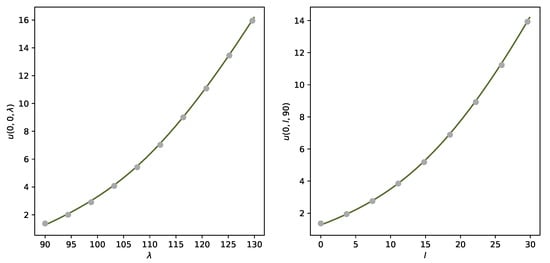
Figure 1. Solution ${\mathcal{U}}_0(l,\lambda )$ for $l=0$, $\lambda \in [90,130]$ (left) and $l\in [0,30]$, $\lambda =90$ (right) computed with the DNN-algorithm (green ine) and reference points computed with Monte Carlo (grey dots).

As a reference for the whole set A, we compute for fixed $(l,\lambda )$ approximate values $U^{MC}(l,\lambda )\approx u(0,l,\lambda )$ with Monte Carlo using ${10}^6$ simulated paths for each point $(l,\lambda )$ (paths are simulated with the Euler-Maruyama scheme). The relative $L^1$-error between the DNN approximation ${\mathcal{U}}_0$ and the MC-solution $U_0^{MC}$ is defined as

$$\begin{array}{c}\hfill ϵ:=\mathbb{E}\left[\left|\frac{{\mathcal{U}}_0({\xi }^l,{\xi }^{\lambda })-U_0^{MC}({\xi }^l,{\xi }^{\lambda })}{U_0^{MC}({\xi }^l,{\xi }^{\lambda })}\right|\right].\end{array}$$

(19)

Using 1000 simulations of ${\xi }^l\sim \mathrm{Unif}\left([0,30]\right),{\xi }^{\lambda }\sim \mathrm{Unif}\left([90,130]\right)$, we obtained a relative error of

$$ϵ=0.0032.$$

(20)

The computation of ${\mathcal{U}}_0$ via the training of a DNN took around 90 s, whereas the computation of $U_0^{MC}$ with Monte Carlo for a fixed point $(l,\lambda )$ took around 4.5 s. This shows that the DNN approach is faster than the MC approach if one wants to compute $u(t,l_i,{\lambda }_i)$ for a grid $(l_i,{\lambda }_i)$ with more than 20 grid points. Details on the numeric implementation and computational equipment are given in Remark 2.

We continue with a more detailed performance analysis for the fixed space point $(l,\lambda )=(0,110)$. As a reference we approximate $u(0,0,110)$ with Monte Carlo using ${10}^7$ simulations. The computation of a single point takes around 2 min, upper and lower bounds for the reference value are $6.2825\mp 0.0033$ ($\mathrm{mean}\mp \tilde{\sigma }/\sqrt{{10}^7}$), where $\tilde{\sigma }$ is the standard deviation of the Monte Carlo simulation. In Table 2 we approximately calculate the mean, the standard deviation, the average relative approximation error (with the Monte Carlo approximation as reference) and the average runtime of ${\mathcal{U}}_0(0,110)$ for different numbers of epochs based on 10 independent realizations (10 independent trainings of ${\mathcal{U}}_0(·,\theta )$).

Table 2. Average value, standard deviation, average relative error of ${\mathcal{U}}_0(0,110)$ and average run time for different number of epochs.

Epochs	Mean	Std. Deviation	Rel. Error	Runtime
1000	6.3126	0.5001	0.0645	17.6
2000	6.3048	0.1151	0.0208	34.9
3000	6.3073	0.1388	0.0189	52.1
4000	6.3360	0.0898	0.0122	69.2
5000	6.3116	0.0468	0.0068	86.3

In Figure 2 we illustrate Log${}_{10}$-average relative error of ${\mathcal{U}}_0(0,110)$ relative to the reference value 6.2825, based on 10 independent realizations. We observe that the relative $L^1$-error decreases with increasing epochs.

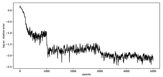
Figure 2. Log${}_{10}$-average relative error of ${\mathcal{U}}_0(0,110)$ relative to the reference value 6.2825, based on 10 independent realizations.

4.2. Computing the CVA for the Reinsurance Contract

The reinsurance company R may default and we denote by ${\tau }_R$ the stopping time representing her default time. If ${\tau }_R\le T$, R will not be able to fulfill her obligations which creates reinsurance counterparty credit risk. The default indicator process $H^R={\left(H_t^R\right)}_{t\ge 0}$ associated with ${\tau }^R$ is given by

$$\begin{array}{c}\hfill H_t^R={\mathbf{1}}_{\{{\tau }_R\le t\}},t\ge 0.\end{array}$$

(21)

We assume that $H^R$ admits a stochastic intensity ${\ell }^R={\left({\ell }_t^R\right)}_{t\ge 0}$ (in the sequel called the default intensity of R), with the property that $H_t^R-{\int }_0^{t\wedge {\tau }_r}{\ell }_s^R\mathrm{d}s$ is a martingale. We assume that ${\ell }^R$ follows the SDE

$$\begin{array}{cc}\hfill \mathrm{d}{\ell }_t^R& ={\mu }^R\left({\ell }_t^R\right)\mathrm{d}t+{\sigma }^R\left({\ell }_t^R\right)(\rho \mathrm{d}{W}_t^1+\sqrt{1-{\rho }^2}\mathrm{d}{W}_t^2),{\ell }_0^R={\ell }_0\in \mathbb{R},\hfill \end{array}$$

(22)

where $W^2$ is a standard Brownian motion independent of $W^1$.

We define the credit value adjustment (CVA) for the reinsurance contract as the market consistent value of the future credit loss, that is,

$$\begin{array}{c}\hfill {CVA}_t=\mathbb{E}\left[{\int }_t^{T}u(s,L_s,{\lambda }_s^L+\gamma {\lambda }_s^L)e^{-r(s-t)}\mathrm{d}{H}_s^R|H_t,L_t,{\lambda }_t^L,{\ell }_t^R\right],0\le t\le T,\end{array}$$

(23)

for $\gamma >0$ and u the value of the insurance contract given in (17). The amount ${CVA}_t$ can be viewed as a risk reserve that the insurance company has to set aside at time t to cover for losses due to reinsurance counterparty risk.

Our framework accounts for two forms of dependence between the default of R and the market value of the insurance contract. First, there is correlation between default intensity ${\ell }^R$ and claim-arrival intensity ${\lambda }^L$, modelled by the parameter $\rho \in [0,1]$, which means that many losses (high claim arrival intensity ${\lambda }^L$) lead to a ess favourable economic outlook for the reinsurance company. Second, there is pricing contagion: at the default time ${\tau }_R$ the risk-neutral claim arrival intensity ${\lambda }^L$ jumps upward in (24), which corresponds to an increase of the market value of the reinsurance contract as the claim arrival intensity becomes larger. This models the phenomenon that the default of R will reduce the supply for reinsurance so that the market price of reinsurance goes up. (This is a pure pricing phenomenon; in particular we do not assume that the claim arrival intensity under the real-world measure jumps upward at ${\tau }^R$).

In [28] it is shown that the value of the CVA is equal to

$$\begin{array}{c}\hfill {CVA}_t=(1-H_t^R)\mathbb{E}\left[{\int }_t^{T}u(s,L_s,{\lambda }_s^L+\gamma {\lambda }_s^L){\ell }_s^R{e}^{-{\int }_t^s(r+{\ell }_u^R)\mathrm{d}u}\mathrm{d}s\mid L_t,{\lambda }_t^L,{\ell }_t^R\right].\end{array}$$

(24)

Moreover, the following PIDE characterization of the CVA is given: It holds that

$$\begin{array}{c}\hfill {CVA}_t=(1-H_t^R)f(t,L_t,{\lambda }_t^L,{\ell }_t^R),\end{array}$$

(25)

where $f:[0,T]\times {\mathbb{R}}^{+}\times \mathbb{R}\times \mathbb{R}\to {\mathbb{R}}^{+}$ is the unique classical solution of the PIDE

$$\begin{array}{cc}\hfill & f_t+{\mathcal{L}}^{(L,{\lambda }^L,{\ell }^R)}f+\ell u(t,l,\lambda +\gamma \lambda )=(\ell +r)f,\hfill \end{array}$$

(26)

for all $(t,l,\lambda ,\ell )\in [0,T)\times {\mathbb{R}}^{+}\times {\mathbb{R}}^2$ with terminal condition $f(T,l,\lambda ,\ell )=0$. The operator ${\mathcal{L}}^{(L,{\lambda }^L,{\ell }^R)}$ is given by

$$\begin{array}{cc}\hfill {\mathcal{L}}^{(L,{\lambda }^L,{\ell }^R)}f=f_{\lambda }{\mu }^L\left(\lambda \right)& +f_{\ell }{\mu }^R(\ell )+\frac{1}{2}{f}_{\lambda \lambda }{\sigma }^L{\left(\lambda \right)}^2+\frac{1}{2}{f}_{\ell \ell }{\sigma }^R{(\ell )}^2+f_{\lambda \ell }\rho {\sigma }^L\left(\lambda \right){\sigma }^R(\ell )\hfill \\ & +{\int }_{{\mathbb{R}}^{+}}(f(t,+z,\lambda ,\ell )-f(t,l,\lambda ,\ell ))\lambda \nu \left(\mathrm{d}z\right),\hfill \end{array}$$

(27)

where f is always evaluated at $(t,l,\lambda ,\ell )$.

We approximate $f(0,l,\lambda ,\ell )$ on the set $B:=\left\{\right(l,\lambda ,\ell ):\in [0,30],\lambda \in [90,130],\ell \in [0,0.05\left]\right\}$ with a deep neural network ${\mathcal{U}}_0^f(l,\lambda ,\ell )$. We use ${\mu }^R(\ell )=(0.05-\ell )$ and ${\sigma }^R(\ell )=0.1\sqrt{\ell }$; the other parameters are as in Section 4.1. Paths of the processes L, ${\lambda }^L$, ${\ell }^R$ are simulated with the Euler-Maruyama scheme on the time grid $0=t_0<t_1<\cdots <t_N=T,\Delta t=T/N$ with $N=20$ and ${({\xi }^l,{\xi }^{\lambda },{\xi }^{\ell })}^T\sim \mathrm{Unif}\left(B\right)$. For each path, we approximate the integral term in (24) with the trapezoidal rule using the endpoints of time grid $0=t_0<t_1<\cdots <t_N=T$. The contract value $u(t_n,·,·)$ is replaced by its neural network approximation ${\mathcal{U}}_n^u$ on the set $A_n:=\{(l,\lambda ):\in [0,30+10n],\lambda \in [90,130]\}$, which we compute as described in Section 4.1 for all $n=0,\cdots ,N$.

In this case study, we are particularly interested in the impact of the correlation parameter $\rho$ and of the pricing contagion parameter $\gamma$ on the CVA. We therefore construct a neural network  ${\mathcal{U}}_0^f(l,\lambda ,\ell ;\rho ,\gamma )$ with additional input variables $\rho$ and $\gamma$. During the training procedure we use different values of $\rho \sim \mathrm{Unif}\left(\right[0,1\left]\right)$ to simulate the paths of ${\ell }^R$ and different values of $\gamma \sim \mathrm{Unif}\left(\right[0,1\left]\right)$ to compute the integral term in (24). In the sequel we write $f^{\rho ,\gamma }$ to stress the dependence of f on $\rho$ and $\gamma$. Figure 3 shows $f^{\rho ,\gamma }(0,l,\lambda ,\ell )$ for varying default-intensity ℓ and Figure 4 for varying $\rho \in [0,1]$ in the left panel and varying $\gamma \in [0,1]$ in the right panel. Moreover, all figures compare the solution for different values of $\gamma$ and $\rho$. We see that ${CVA}_0$ increases in both $\rho$ and $\gamma$, but the effect of price contagion (i.e., variation in $\gamma$) is quite pronounced and dominates the effect of dependence between intensities (i.e., variation in $\rho$).

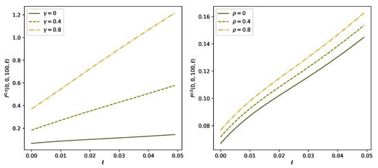
Figure 3. Solution $f^{\rho ,\gamma }(0,l,\lambda ,\ell )$ for $l=0$, $\lambda =100$, varying $\ell \in [0,0.05]$ and different levels of $\gamma$ and $\rho$ with computed with the DNN-algorithm. We have $\rho =0$ (left) resp. $\gamma =0$ (right).

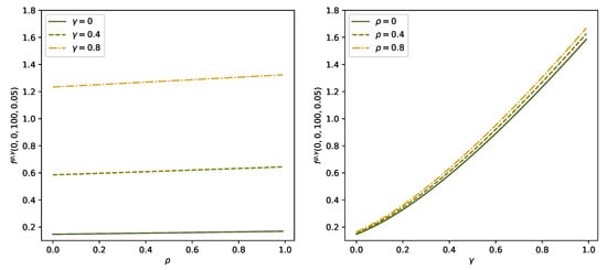
Figure 4. Solution ${}^{\rho ,\gamma }(0,l,\lambda ,\ell )$ for $l=0$, $\lambda =100$, $\ell =0.05$ varying $\rho \in [0,1]$ and different levels of $\gamma$ (left) and varying $\gamma \in [0,1]$ for different levels of $\rho$ (right) computed with the DNN-algorithm.

This part of the case study highlights the computational advantages of the DNN approach compared with nested Monte Carlo methods. Figure 5 shows $f^{\rho ,\gamma }(0,l,\lambda ,\ell )$ for varying claim-arrival intensity $\lambda$ together with reference solution points computed with classical Monte Carlo simulations. In this nested Monte Carlo problem, we use 3000 simulations to approximate the inner function u and 2000 path simulations for the outer expectation. The integral term is approximated following the trapezoidal rule on the time grid $0=t_0<t_1<\cdots <t_N=T$. Computation of only one point takes more than 5 min (despite using only 3000 resp. 2000 simulations). On the other hand training the network approximations of $u(t_n,·,·)$ for all $n=0,\cdots ,N-1$ takes around 20 min and training of the network approximation for $f(0,·,·,·)$ takes ess than 4 min, i.e., it takes only around 24 min to train the network for the whole space domain B and for all values of $\rho ,\gamma \in [0,1]$. This should be contrasted with a computation time of more than 60 min to compute the CVA for only 12 space points (numerical details on the training procedure are given in Remark 2). Due to the computational infeasibility of nested Monte Carlo solutions, we omit a similar error analysis as in (19).

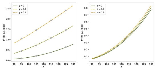
Figure 5. Solution $f^{\rho ,\gamma }(0,l,\lambda ,\ell )$ for $l=0$, $\ell =0.05$ varying $\lambda \in [90,130]$, different levels of $\gamma$ resp. $\rho$ and $\rho =0$ resp. $\gamma =0$ (left resp. right) computed with the DNN-algorithm. The reference points are computed with Monte Carlo (left, grey dots).

In [28] we moreover addressed the hedging of RCCR by dynamic trading in a credit default swap (CDS) on the reinsurance company using a quadratic hedging approach. The computation of the mean-variance minimizing hedging strategies (Theorem 4.3 [28]) involves computing various derivatives of the functions f and g, where g is the present value of future payments of the CDS. The DNN algorithm is particularly useful for this: we can approximate f and g for $0=t_0<\cdots <t_N=T$ with neural networks on the whole space domain and compute their derivatives via automatic differentiation. In [28] the derivatives of f and g were computed via classical Monte Carlo, which fairly unstable and time-consuming.

Remark 2

(Details regarding the numerical implementation). Our choice of the network architecture largely follows [15]. Throughout, we use DNNs with 2 hidden ayers and 20 nodes for the hidden ayers. For a payoff of the form (16), it is advantageous to use softplus as activation function for the hidden ayers and the identity for the output ayer. The networks are initialized with random numbers using the Xavier initialization. We use mini-batch optimization with mini-batch size $M=3000$, batch normalization and 5000 epochs for training. We minimize the loss function with the Adam optimizer and decrease learning rate from 0.1 to 0.01 and 0.001 after a 1000 and 3000 epochs. The neural networks used are standard, hence, training induces a cost that is inear in M and e, i.e., $\mathcal{O}\left(Me\right)$, where M is the batch size and e the number of epochs, see also Table 2 in the column runtime. Each of the numerical experiments presented in this paper are performed in Python using Tensorflow computations on a Lenovo Thinkpad notebook with an Intel Core i5 processor (1.7 GHz) and 16 GB memory. Note that one can gain a performance boost by using GPU computing, e.g., with Cuda from Nvidia, but to emphasize the practicality of the algorithm we run our computations with a standard CPU.

Remark 3

(Further examples for the inear case). Further examples for the inear case can be found in our companion papers [22,29]. In [22] we consider an example from [30], who study the pricing of basket options in jump diffusion models. In [29] we compute the ruin probability for an insurance company with three different business ines, which leads to a boundary value problem. In both cases the performance of the deep learning method is assessed by comparing the solution to the results of an extensive Monte Carlo simulation. The DNN algorithm performed well in all cases considered.

5. Deep Learning Approximation for Semilinear PIDEs

Next we consider semilinear PIDEs of the form

$$\begin{array}{cc}\hfill u_t(t,x)& +\mathcal{L}u(t,x)+f(t,x,u(t,x),\nabla u(t,x\left)\right)=0,(t,x)\in [0,T)\times D,\hfill \\ \hfill u(t,x)& =g(t,x),(t,x)\in \left([0,T)\times ({\mathbb{R}}^d \backslash \{D)\right)\cup \left(\left\{T\right\}\times {\mathbb{R}}^d\right).\hfill \end{array}$$

(28)

Here, $f:[0,T]\times {\mathbb{R}}^d\times \mathbb{R}\times {\mathbb{R}}^d\to \mathbb{R}$ is a nonlinear function and the integro-differential operator $\mathcal{L}$ is given in (3). Our goal is to extend the deep splitting approximation method developed by [14] for semilinear PDEs without boundary conditions to the more general PIDE (28). Moreover, we propose an approach for improving the performance of the method. In order to derive the method with a minimal amount of technicalities, we assume that a classical solution of this PIDE exists. Note however, that the deep splitting approximation applies also in cases where the PIDE (28) admits only a continuous viscosity solution. In that case one has to consider the forward backward stochastic differential equation associated with (28), see see [22] or [17]. The very recent contribution [21] considers an extension of the deep splitting to PIDEs of the form (28) with Neumann boundary conditions, but assumes that f is independent of the gradient of u.

5.1. Basic Method

We divide the interval $[0,T]$ into subintervals using a time grid $0=t_0<t_1<\cdots <t_N=T$ and we et $\Delta t_n=t_n-t_{n-1}$. Suppose that $u^{*}$ is the unique solution of the PIDE (28). Define for a fixed $u\in {\mathcal{C}}^{0,1}([0,T]\times D)$ the function

$$(t,x)\mapsto f_{\left[u\right]}(t,x)=f(t,x,u(t,x),\nabla u(t,x)).$$

Then $u^{*}$ also solves the inear PIDE

$$\begin{array}{c}\hfill u_t(t,x)+\mathcal{L}u(t,x)+f_{\left[u^{*}\right]}(t,x)=0.\end{array}$$

(29)

Applying the Feynman-Kac formula to the inear PIDE (29), we get the following representation for $u^{*}$

$$\begin{array}{c}\hfill u^{*}(t_{n-1},x)=\mathbb{E}\left[u^{*}(t_n\wedge \tau ,X_{t_n\wedge \tau }^x)+{\int }_{t_{n-1}}^{t_n\wedge \tau }{f}_{\left[u^{*}\right]}(s,X_s^x)\mathrm{d}s\right],x\in D.\end{array}$$

(30)

Here, $X^x$ solves the SDE (1) with initial condition $X_{t_{n-1}}^x=x$, that is,

$$\begin{array}{c}\hfill X_t^x=x+{\int }_{t_{n-1}}^t\mu (s,X_s^x)\mathrm{d}s+{\int }_{t_{n-1}}^t\sigma (s,X_s^x)\mathrm{d}{W}_s+{\int }_{t_{n-1}}^t{\int }_{{\mathbb{R}}^d}\gamma (s,X_{s-}^x,z)J(\mathrm{d}z,\mathrm{d}s),\end{array}$$

(31)

and the stopping time $\tau$ is given by $\tau =inf\{s>t_{n-1}:X_s^x\notin D\}$. In the deep splitting method proposed in [14] the integral term in (30) is approximated by the endpoint rule

$$\begin{array}{c}\hfill {\int }_{t_{n-1}}^{t_n}{f}_{\left[u^{*}\right]}(s,X_s^x)\mathrm{d}s\approx f_{\left[u^{*}\right]}(t_n,X_{t_n}^x)\Delta t_n.\end{array}$$

(32)

An approximate solution ${\mathcal{U}}_n(·)\approx u^{*}(t_n,·)$, $n=0,\cdots N$ is then found by backward induction over the grid points. The solution at the maturity $t_N=T$ is defined using the terminal condition, that is, ${\mathcal{U}}_N\left(x\right):=g(T,x).$ Given ${\mathcal{U}}_n$, we then compute ${\mathcal{U}}_{n-1}$, $n=1,2,\cdots ,N$ as follows. First, we put

$$\begin{array}{cc}\hfill \tilde{u}(t_{n-1},x)& :=\mathbb{E}[{\mathcal{U}}_n\left(X_{t_n}^x\right){\mathbf{1}}_{\{\tau >t_n\}}+g(\tau ,X_{\tau }^x){\mathbf{1}}_{\{\tau \le t_n\}}\hfill \\ & +(t_n\wedge \tau -t_{n-1})f\left(t_n\wedge \tau ,X_{t_n\wedge \tau }^x,{\mathcal{U}}_n\left(X_{t_n\wedge \tau }^x\right),\nabla {\mathcal{U}}_n\left(X_{t_n\wedge \tau }^x\right)\right)].\hfill \end{array}$$

(33)

Then, we compute ${\mathcal{U}}_{n-1}\approx \tilde{u}(t_{n-1},·)$ by applying the regression-based DNN algorithm method from Section 3. In this step, it is important to work with DNNs with a smooth activation function so that $\nabla {\mathcal{U}}_n$ is well-defined (If $g(T,·)$ is not ${\mathcal{C}}^1$ one has to define ${\mathcal{U}}_N$ as DNN approximation to the terminal condition; see for instance [17]).

Remark 4.

An additional complication may arise if the domain D is unbounded. In that case, we compute the approximate solution on some bounded set $A_n\subset D$. We have to make sure that the set $A_n$ is big enough so that the probability of generating paths with $X_{t_{n-1}}\in A_{n-1}$ but $X_{t_n}\notin A_n$ is sufficiently small. Then, these paths can be ignored without affecting the training procedure. There are various ways to achieve this, see [14] for details.

5.2. Alternative Method

Next, we discuss an alternative linearization procedure based on the midpoint rule

$$\begin{array}{c}\hfill {\int }_{t_{n-1}}^{t_n}{f}_{\left[u^{*}\right]}(s,X_s^x)\mathrm{d}s\approx f_{\left[u^{*}\right]}\left({\overline{t}}_n,X_{{\overline{t}}_n}^x)\right)\Delta t_n.\end{array}$$

(34)

Here, ${\overline{t}}_n=(t_{n-1}+t_n)/2$ is the midpoint of the interval $[t_{n-1},t_n]$. It is well known that (34) usually provides a better approximation to an integral than the endpoint rule (32). We therefore propose the following approximation scheme based on the midpoint rule. In a first step, we apply the approximation (33) over the smaller interval $[{\overline{t}}_n,t_n]$; this yields an approximate solution ${\overline{\mathcal{U}}}_n$ at ${\overline{t}}_n$. Next, we define

$$\begin{array}{cc}\hfill \tilde{u}(t_{n-1},x)& :=\mathbb{E}[{\mathcal{U}}_n\left(X_{t_n}^x\right){\mathbf{1}}_{\{\tau >t_n\}}+g(\tau ,X_{\tau }^x){\mathbf{1}}_{\{\tau \le t_n\}}\hfill \\ & +(t_n\wedge \tau -t_{n-1})f\left({\overline{t}}_n\wedge \tau ,X_{{\overline{t}}_n\wedge \tau }^x,{\overline{\mathcal{U}}}_n\left(X_{{\overline{t}}_n\wedge \tau }^x\right),\nabla {\overline{\mathcal{U}}}_n\left(X_{{\overline{t}}_n\wedge \tau }^x\right)\right)];\hfill \end{array}$$

(35)

as before, a numerical approximation ${\mathcal{U}}_{n-1}$ to $\tilde{u}(t_{n-1},x)$ is computed via the deep learning algorithm from Section 3. Our numerical experiments in Section 6 show that the approximation based on the midpoint rule performs significantly better than the original deep splitting method from [14].

Remark 5

(Convergence results for the semilinear case). The companion paper [22] provides a convergence result for semilinear Cauchy problems of the form (28) as well. The approximation error is divided into three components: the Euler approximation error from the time discretization (which is of order $\Delta t_m$), an error due to the linearization of the equation and finally an approximation error in the class of neural networks considered. A precise formulation is more involved than in the inear case and we refer to [22] for details.

6. Case Study for the Semilinear Case: Optimal Credit Portfolios with Risk Capital Constraints

As a case study for the semilinear case, we consider the problem of optimizing the size of the credit portfolio of a financial institution under transaction costs and risk capital constraints. Without capital constraints, the problem admits an analytic solution and is therefore a useful test case. With capital constraints, the model leads to a semilinear boundary value problem for which there is no explicit solution, and we study this case numerically using the deep splitting method. In fact, the analysis of the impact of risk capital constraints on optimal credit portfolios is also interesting in its own right.

We consider a stylized model of a financial institution who invests in a credit portfolio with market value $S_t$ at time t and in cash. We assume that the process S has dynamics

$$\mathrm{d}{S}_t=\overline{\mu }\mathrm{d}t+\sigma \mathrm{d}{W}_t-\mathrm{d}{R}_t,$$

Here, the Brownian motion W models the compensated small credit losses, the compound Poisson process R with intensity $\lambda$ and jump size distribution $\eta \left(\mathrm{d}z\right)$ models the large credit losses, and $\overline{\mu }>0$ is the expected return earned by the portfolio. We assume that the credit portfolio can be adjusted only gradually over time. In mathematical terms, this means that the financial institution uses an absolutely continuous trading strategy with trading rate $\theta ={\left({\theta }_t\right)}_{0\le t\le T}$, so that for a given strategy $\theta$, the size $Q^{\theta }$ of the portfolio satisfies $\mathrm{d}{Q}_t^{\theta }={\theta }_t\mathrm{d}t$. Moreover, the financial institution incurs a transaction cost, that is proportional to the trading rate ${\theta }_t^2$. This models the fact that a rapid adjustment of the portfolio is expensive, as the institution needs to carry out costly marketing activities or enter into expensive securitization activities. Given a parameter $\kappa >0$ modelling the size of the transaction cost, the cash position $C^{\theta }$ has dynamics

$$\mathrm{d}{C}_t^{\theta }=-\left({\theta }_t{S}_t+\kappa {\theta }_t^2\right)\mathrm{d}t.$$

Here, the term $-{\theta }_t{S}_t\mathrm{d}t$ gives the revenue from trading the credit portfolio and the term $-\kappa {\theta }_t^2\mathrm{d}t$ models the reduction of the cash position due to transaction costs. From a mathematical viewpoint, this model is fairly similar to models used in the iterature on optimal portfolio execution such as [31] or [32].

Denote by $E_t^{\theta }=S_t{Q}_t^{\theta }+C_t^{\theta }$ the institution’s equity. We assume that the institution wants to maximize the expected value of her equity position $E_T^{\theta }$ at some horizon date time T, and that she incurs a liquidation cost of size $\gamma {\left(Q_T^{\theta }\right)}^2$ for some parameter $\gamma >0$. Note that for a given strategy $\theta$ the process $(Q^{\theta },E^{\theta })$ has dynamics

$$\begin{array}{cc}\hfill \mathrm{d}{Q}_t^{\theta }& ={\theta }_t\mathrm{d}t,\hfill \\ \hfill \mathrm{d}{E}_t^{\theta }& =Q_t^{\theta }\overline{\mu }\mathrm{d}t+Q_t^{\theta }\sigma \mathrm{d}{W}_t-Q_t^{\theta }\mathrm{d}{R}_t-\kappa {\theta }_t^2\mathrm{d}t.\hfill \end{array}$$

(36)

Hence, the pair $(Q^{\theta },E^{\theta })$ is Markov and we may use this process as state process. We define the value function of the optimization problem for $t\in [0,T]$ as

$$\begin{array}{c}\hfill u(t,q,e):=\underset{\theta \in \mathcal{A}}{sup}\mathbb{E}\left[E_T^{\theta }-\gamma {\left(Q_T^{\theta }\right)}^2\mid Q_t^{\theta }=q,E_t^{\theta }=e\right],\end{array}$$

(37)

where $\mathcal{A}$ denotes the set of all adapted trading rates such that $E\left[{\int }_0^T{\theta }_t^2\mathrm{d}t\right]<\infty$.

To prevent early ruin, financial regulators usually impose risk capital constraints. In particular, they may liquidate a financial institution if the equity is too low compared to the size or riskiness of the institution’s credit portfolio. Below, we use the deep splitting method to study how capital constraints affects the value function and the optimal strategy of the financial institution. First, we consider the unconstrained problem for which there is an explicit solution of the HJB equation (PIDE (40) below), which can be used to test the performance of the deep splitting method. Details on the numerical implementation and the computational equipment are given in Remark 6.

6.1. The Case without Constraints

By standard arguments, the HJB equation associated with the problem (37) is

$$\begin{array}{cc}\hfill u_t(t,q,e)& +q\overline{\mu }{u}_e(t,q,e)+\frac{1}{2}{\sigma }^2{q}^2{u}_{ee}(t,q,e)+\lambda {\int }_0^{\infty }[u(t,q,e+qz)-u(t,q,e)]\eta \left(\mathrm{d}z\right)\hfill \\ & +\underset{\theta \in \mathbb{R}}{sup}\{\theta u_q(t,q,e)-\kappa {\theta }^2{u}_e(t,q,e)\}=0,\hfill \end{array}$$

(38)

with terminal condition $u(T,q,e)=e^2-\gamma q^2$. Maximization gives the candidate optimal trading rate

$$\begin{array}{c}\hfill {\theta }_t^{*}(t,q,e)=\frac{1}{2\kappa }\frac{u_q(t,q,e)}{u_e(t,q,e)};\end{array}$$

(39)

substitution into (38) yields the semilinear PIDE

$$\begin{array}{cc}\hfill u_t(t,q,e)& +q\overline{\mu }{u}_e(t,q,e)+\frac{1}{2}{\sigma }^2{q}^2{u}_{ee}(t,q,e)+\lambda {\int }_0^{\infty }[u(t,q,e+qz)-u(t,q,e)]\eta \left(\mathrm{d}z\right)\hfill \\ & +\frac{1}{4\kappa }\frac{u_q{(t,q,e)}^2}{u_e(t,q,e)}=0.\hfill \end{array}$$

(40)

To solve the case without constraints, we make the Ansatz $u(t,q,e)=e+v(t,q)$, that is, we assume that u is inear in the equity value e. This implies

$$\lambda {\int }_0^{\infty }[u(t,q,e+qz)-u(t,q,e)]\eta \left(\mathrm{d}z\right)=\lambda q{\int }_0^{\infty }z\eta \left(\mathrm{d}z\right)=:q\lambda \overline{\eta }.$$

If we define $\overline{\alpha }=\overline{\mu }-\lambda \overline{\eta }$, (40) reduces to the following first order PDE for v

$$\begin{array}{c}\hfill -\overline{\alpha }q=v_t(t,q)+\frac{v_q{(t,q)}^2}{4\kappa },\end{array}$$

(41)

with terminal condition $v(T,q)=-\gamma q^2$. To find an explicit solution for v, we follow [31] and make the Ansatz $v(t,q)=h_0\left(t\right)+h_1\left(t\right)q-\frac{1}{2}{h}_2\left(t\right)q^2.$ Substitution in the HJB Equation (41) gives the following ODE system for $h_0,h_1,h_2$

$$\begin{array}{c}\hfill h_2^{\prime }=h_2^2/\left(2\kappa \right),h_1^{\prime }=-\overline{\alpha }+h_1{h}_2/\left(2\kappa \right),h_0^{\prime }=-h_1^2/\left(4\kappa \right)\end{array}$$

(42)

with terminal condition $h_0\left(T\right)=h_1\left(T\right)=0$ and $h_2\left(T\right)=2\gamma$. The ODEs can be solved explicitly: one has

$$\begin{array}{cc}\hfill h_2\left(t\right)& =\frac{2\kappa }{T+\frac{\kappa }{\gamma }-t},\hfill \end{array}$$

(43)

$$\begin{array}{cc}\hfill h_1\left(t\right)& =\frac{c_1+\frac{1}{2}\overline{\alpha }{t}^2-a\overline{\alpha }t}{a-t},\mathrm{where}{c}_1:=-\frac{1}{2}\overline{\alpha }{T}^2+a\overline{\alpha }T\mathrm{and}a:=T+\frac{\kappa }{\gamma },\hfill \end{array}$$

(44)

$$\begin{array}{cc}\hfill h_0\left(t\right)& =\frac{1}{4\kappa (a-t)}\left(-\frac{2}{3}{\overline{\alpha }}^2{a}^4+\frac{2}{3}{\overline{\alpha }}^2{a}^{3}t+2\overline{\alpha }{a}^2{c}_1+\overline{\alpha }{c}_1{t}^2-2\overline{\alpha }a{c}_{1}t-c_1^2+\frac{1}{12}{\overline{\alpha }}^2{t}^4-\frac{1}{3}{\overline{\alpha }}^{2}a{t}^3\right).\hfill \end{array}$$

(45)

For comparison purposes we computed the solution $u(t,x)=u(t,q,e)$ of (40) with the deep splitting algorithm on the set A:=$\left\{\right(q,e):-7\le q\le 7,0\le e\le 6\}$. For this we partition the time horizon into $N=10$ intervals $0=t_0<t_1<\cdots <t_N=T$ and simulate the auxiliary process $X=(X^Q,X^E)$ with $X_t^Q={\xi }^Q$ and

$$\begin{array}{cc}\hfill X_t^E& ={\xi }^E+{\int }_{t_{n-1}}^t{X}_s^Q\overline{\mu }\mathrm{d}s+{\int }_{t_{n-1}}^t{X}_s^Q\sigma \mathrm{d}{W}_s+{\int }_{t_{n-1}}^t{\int }_{\mathbb{R}}{X}_s^{Q}zJ(\mathrm{d}z,\mathrm{d}s),\hfill \end{array}$$

(46)

where $\xi =({\xi }^Q,{\xi }^E)$ is uniformly distributed on $[-7,7]\times [0,7]$, W is a Brownian motion and J is a jump measure with compensating measure $\nu =\lambda \eta$ for $\eta$ a Gamma distribution with parameters $\alpha$ and $\beta$. Moreover, we identify the nonlinear term in the PIDE as

$$\begin{array}{c}\hfill f(t,x,y,z)=\frac{1}{4\kappa }\frac{z_1^2}{z_2}.\end{array}$$

(47)

We used the midpoint rule (34) to linearize the PIDE. The network architecture was as in Remark 6. The training for the whole network consisting of 20 subnetworks (a DNN for every grid point $t_n$, $0\le n\le 9$ and a DNN for every midpoint ${\overline{t}}_n$) took around 4400 s. Table 3 contains the parameters used in the experiment. Figure 6 shows the approximate solution ${\mathcal{U}}_0$ obtained by the deep splitting algorithm (solid ine) and the analytic reference solution (dashed ine) for varying $q\in [-7,7]$ in the left panel and varying $e\in [0,6]$ in the right panel.

Table 3. Parameters for the credit optimization problem.

$\mathit{\sigma }$	$\mathit{\gamma }$	$\mathit{\kappa }$	$\overline{\mathit{\mu }}$	$\mathit{\lambda }$	$\mathit{\alpha }$	$\mathit{\beta }$
$0.1$	$0.1$	$0.1$	$0.8$	5	$0.4$	4

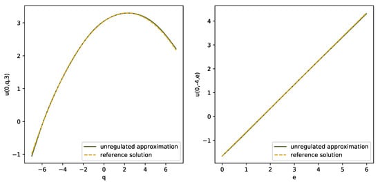
Figure 6. Solution of the unconstrained credit optimization problem for $q\in [-7,7]$, $e=3$ (left) and $q=-4$, $e\in [0,6]$ (right) with the DNN-algorithm (green) and reference solution (orange).

As the solution u can be zero, we report the absolute $L^1$-error between the DNN approximation ${\mathcal{U}}_n$ and the analytic solution, that is, ${\epsilon }_{t_n}^{\mathrm{abs}}:=\mathbb{E}\left[\left|{\mathcal{U}}_n\left(\xi \right)-u(t_n,\xi )\right|\right].$ To compute the absolute error, we used 10,000 simulations of $\xi =({\xi }^Q,{\xi }^E)$ where ${\xi }^Q\sim \mathrm{Unif}\left([-7,7]\right)$ and ${\xi }^E\sim \mathrm{Unif}\left([0,6]\right)$. Figure 7 illustrates the mean ${\epsilon }_{t_n}^{\mathrm{abs}}$ of 10 different DNN approximations ${\mathcal{U}}_n^i,i=1,\cdots ,10$ for each time point $t_n$, $n=0,\cdots ,N-1$ using once the midpoint rule (solid ine) and once the original method from [14] (dashed ine). We see that the algorithm based on the midpoint rule performs substantially better than the original deep splitting method.

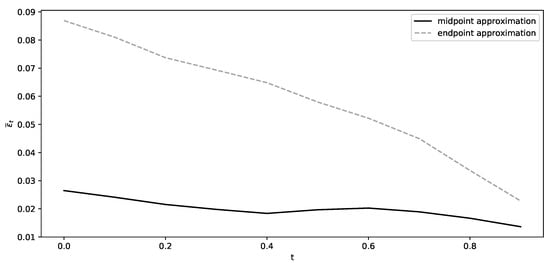
Figure 7. Comparison of the two different training methods illustrating the averaged absolute $L^1$-error ${\overline{\epsilon }}_t^{\mathrm{abs}}$ using endpoint (grey) and midpoint (black) approximation in 10 training procedures.

6.2. The Optimization Problem with Constraints

Next, we discuss the optimization problem under risk capital constraints. We expect that risk capital constraints will alter the investment decisions of the financial institution since she wants to avoid liquidation of the company. To set up the corresponding optimization problem, we need to specify the set D of acceptable positions of the financial institution and the liquidation value given that her position exits from D. For numerical reasons, it is convenient to model D as a bounded set. Given large constants $\overline{e}$ and $\overline{q}$ and a parameter $\delta >0$, we define the set D of acceptable positions as

$$\begin{array}{c}\hfill D=\{(q,e)\in {\mathbb{R}}^2:|q|<\overline{q},\delta |q|<e<\overline{e}\}.\end{array}$$

(48)

The constraint $e>\delta \left|q\right|$ implies that before liquidation the solvency ratio $|Q_t|/E_t$ of the institution is bounded by ${\delta }^{-1}$, so that ${\delta }^{-1}$ can be viewed as a measure of the regulator’s risk tolerance. We assume that the liquidation value of the portfolio on the boundary of D is given by the value $u^{\mathrm{unreg}}$ of the unconstrained problem, reduced by a penalty $k(t,q,e)\ge 0$, and we set

$$g(t,q,e)=u^{\mathrm{unreg}}(t,q,e)-k(t,q,e).$$

Here, $k:[0,T]\times [-\overline{q},\overline{q}]\times [0,\overline{e}]\to [0,\infty )$ is a smooth function that penalizes exit from the set of acceptable positions. We assume that $k(t,q,\overline{e})=0,0\le t\le T$ (no penalization for high equity values) and that $k(T,q,e)=0,0\le e\le \overline{e}$ (no penalization at maturity). In our numerical experiments, we take $\overline{e}={10}^6$, $\delta =1$, and $k(t,q,e)=0.5(T-t)(\overline{e}-e)/\overline{e}$; the other parameters are identical to the unconstrained case, see Table 3.

The value function for the problem with risk capital constraints is

$$\begin{array}{c}\hfill u^{\mathrm{reg}}(t,q,e)=\underset{\theta \in \mathcal{A}}{sup}\mathbb{E}\left[g(\tau \wedge T,Q_{\tau \wedge T}^{\theta },E_{\tau \wedge T}^{\theta })|Q_t=q,E_t=e\right],t\in [0,T],(q,e)\in D,\end{array}$$

(49)

where $\tau =inf\{s\ge t:(Q^{\theta },E^{\theta })\notin D\}$. The PIDE associated with this control problem and the form of the optimal strategy are the same as in the unregulated case (see (38) and (39)), but now we have in addition the boundary condition

$$u(t,q,e)=u^{\mathrm{unreg}}(t,q,e)-k(t,q,e),t\in [0,T),(q,e)\notin D.$$

Due to the boundary condition, the Ansatz $u^{\mathrm{reg}}(t,q,e)=e+v(t,q)$ does not hold and we have to compute $u^{\mathrm{reg}}$ via the deep splitting algorithm. In view of its superior performance in the unconstrained case, we worked with the midpoint procedure, and we used the same network architecture as in the unconstrained case. We worked on the set $A=\left\{\right(q,e):-e\le q\le e,0\le e\le 6\}\subset D$. Figure 8 illustrates the DNN-approximation for $u^{\mathrm{reg}}(0,q,e)$ (solid ine) and $u^{\mathrm{unreg}}(0,q,e)$ (dashed ine) on the sections $\left\{\right(q,4):q\in [-4,4\left]\right\}$ (left panel) and $\left\{\right(2,e):e\in [2,6\left]\right\}$ (right panel). The right plot shows that with risk capital constraints the value function is concave in e and for $e\approx 2$ significantly lower than $u^{\mathrm{unreg}}$ (for $\delta =1$ the point $(q,e)=(2,2)$ belongs to the lower bound of D).

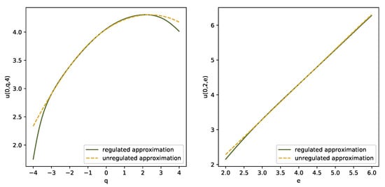
Figure 8. DNN-approximations of $u^{reg}(0,q,e)$ (green) and $u^{unreg}(0,q,e)$ (orange) on the section $\left\{\right(q,4):q\in [-4,4\left]\right\}$ (left) and on $\left\{\right(2,e):e\in [2,6\left]\right\}$ (right).

The optimal trading rate is plotted in Figure 9. The plots show that the optimal strategy for the regulated case (solid ine) differs from the optimal strategy in the unregulated case (dashed ine), as the financial institution wants to reduce the size $\left|q\right|$ of her risky position in order to avoid costly liquidation, in particular when her position is close to the liquidation boundary. For instance, in the right plot the optimal trading rate for $q=2$ is negative for e close to 2.

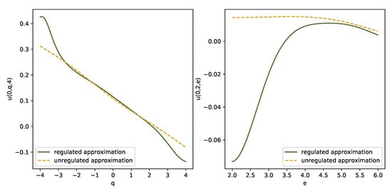
Figure 9. DNN-approximations of the optimal strategy ${\theta }_0^{*}$ for the regulated case (green) and the unregulated case (orange) on $\left\{\right(q,4):q\in [-4,4\left]\right\}$ (left) and on $\left\{\right(2,e):e\in [2,6\left]\right\}$ (right).

Remark 6

(Details on the numerical implementation). We used a similar network architecture as in [14]. We worked with deep neural networks with 2 hidden ayers consisting of 100 nodes each. All neural networks are initialized with random numbers using the Xavier initialization. We use mini-batch optimization with mini-batch size $M=5000$, batch normalization and 12,000 training epochs. The loss function is minimized with the Adam optimizer and decreasing learning rate from 0.1 to 0.01, 0.001, 0.0001 and 0.00001 after 2000, 4000, 6000 and 8000 epochs. We use sigmoid as activation function for the hidden ayers and theidentity for the output ayer. The neural networks used are standard, and, hence, training induces a cost that is inear in M, e and N, i.e., $\mathcal{O}\left(NMe\right)$, where M is the batch size, e the number of epochs and N is the size of the time discretization. All computations are performed in Python using Tensorflow computations on a Lenovo Thinkpad notebook with an Intel Core i5 processor (1.7 GHz) and 16 GB memory.

Remark 7

(Further examples for the semilinear case). For an additional application of our DNN-algorithm to a semilinear PIDE, we refer to the companion paper [22] where the semilinear stochastic inear regulator problem is studied. It is well known that there exists an analytical solution (e.g., see [33]), that can be used to verify the accuracy of the numerical method. However, there are not many (non-trivial) semilinear problems of type (7) with an explicit solution, and the majority of standard numerical methods is quite involved, so that it is not straightforward to come up with further test cases.

7. Conclusions

In this paper we studied an extension of the regression-based deep neural network algorithms of [14,15,17] to PIDE problems from insurance and finance. We illustrated the performance of our methodology, carrying out extensive tests for several multi-dimensional PIDEs arising in typical financial or actuarial pricing and control problems. In all test cases, the performance of the proposed approximation algorithms was satisfying in terms of accuracy and speed. Our results suggest that deep neural network algorithms might become a useful enhancement of the toolbox for solving many valuation and control problems in insurance and finance.

We continue with some ideas for further research. A possible alternative to the methodology proposed in this paper is to extend some of the deep backward dynamic programming schemes discussed in [17] to the PIDE case, similarly as in [18]. However, instead of approximating the increment $u(t_n,x+\Delta x)-u(t_n,x)$ by a third (large) network, one might use the solution at time $t_{n+1}$ as this is ess involved numerically. Moreover, it might be interesting to extend the method to the more general class of fully nonlinear PIDEs.

References

- Cont, R.; Voltchkova, E. A finite difference scheme for option pricing in jump diffusion and exponential Lévy models. SIAM J. Numer. Anal. 2005, 43, 1596–1626. [Google Scholar] [CrossRef]
- Andersen, L.; Andreasen, J. Jump-diffusion processes: Volatility smile fitting and numerical methods for option pricing. Rev. Deriv. Res. 2000, 4, 231–262. [Google Scholar] [CrossRef]
- Matache, A.M.; Von Petersdorff, T.; Schwab, C. Fast deterministic pricing of options on Lévy driven assets. ESAIM Math. Model. Numer. Anal. 2004, 38, 37–71. [Google Scholar] [CrossRef]
- Kwon, Y.; Lee, Y. A second-order finite difference method for option pricing under jump-diffusion models. SIAM J. Numer. Anal. 2011, 49, 2598–2617. [Google Scholar] [CrossRef]
- Briani, M.; Natalini, R.; Russo, G. Implicit–explicit numerical schemes for jump–diffusion processes. Calcolo 2007, 44, 33–57. [Google Scholar] [CrossRef]
- Giles, M.B. Multilevel Monte Carlo path simulation. Oper. Res. 2008, 56, 607–617. [Google Scholar] [CrossRef]
- Glasserman, P. Monte Carlo Methods in Financial Engineering; Springer: New York, NY, USA, 2003. [Google Scholar]
- Metwally, S.A.; Atiya, A.F. Using Brownian bridge for fast simulation of jump-diffusion processes and barrier options. J. Deriv. 2002, 10, 43–54. [Google Scholar] [CrossRef][Green Version]
- Han, J.; Jentzen, A.; Weinan, E. Solving high-dimensional partial differential equations using deep learning. Proc. Natl. Acad. Sci. USA 2018, 115, 8505–8510. [Google Scholar] [CrossRef]
- Han, J.; Jentzen, A. Deep learning-based numerical methods for high-dimensional parabolic partial differential equations and backward stochastic differential equations. Commun. Math. Stat. 2017, 5, 349–380. [Google Scholar] [CrossRef]
- Han, J.; Long, J. Convergence of the deep BSDE method for coupled FBSDEs. Probab. Uncertain. Quant. Risk 2020, 5, 5. [Google Scholar] [CrossRef]
- Kremsner, S.; Steinicke, A.; Szölgyenyi, M. A deep neural network algorithm for semilinear elliptic PDEs with applications in insurance mathematics. Risks 2020, 8, 136. [Google Scholar] [CrossRef]
- Huré, C.; Pham, H.; Warin, X. Deep backward schemes for high-dimensional nonlinear PDEs. Math. Comput. 2020, 89, 1547–1579. [Google Scholar] [CrossRef]
- Beck, C.; Becker, S.; Cheridito, P.; Jentzen, A.; Neufeld, A. Deep splitting method for parabolic PDEs. SIAM J. Sci. Comput. 2021, 43, A3135–A3154. [Google Scholar] [CrossRef]
- Beck, C.; Becker, S.; Grohs, P.; Jaafari, N.; Jentzen, A. Solving the Kolmogorov PDE by means of deep learning. J. Sci. Comput. 2021, 88, 73. [Google Scholar] [CrossRef]
- Pham, H.; Warin, X.; Germain, M. Neural networks-based backward scheme for fully nonlinear PDEs. SN Partial. Differ. Equ. Appl. 2021, 2, 16. [Google Scholar] [CrossRef]
- Germain, M.; Pham, H.; Warin, X. Approximation error analysis of some deep backward schemes for nonlinear PDEs. SIAM J. Sci. Comput. 2022, 44, A28–A56. [Google Scholar] [CrossRef]
- Castro, J. Deep Learning Schemes For Parabolic Nonlocal Integro-Differential Equations. arXiv 2021, arXiv:2103.15008. [Google Scholar] [CrossRef]
- Al-Aradi, A.; Correia, A.; Naiff, D.d.F.; Jardim, G.; Saporito, Y. Applications of the Deep Galerkin Method to Solving Partial Integro-Differential and Hamilton-Jacobi-Bellman Equations. arXiv 2019, arXiv:1912.01455. [Google Scholar]
- Sirignano, J.; Spiliopoulos, K. DGM: A deep learning algorithm for solving partial differential equations. J. Comput. Phys. 2018, 375, 1339–1364. [Google Scholar] [CrossRef]
- Boussange, V.; Becker, S.; Jentzen, A.; Kuckuck, B.; Pellissier, L. Deep learning approximations for non-local nonlinear PDEs with Neumann boundary conditions. arXiv 2022, arXiv:2205.03672. [Google Scholar]
- Frey, R.; Köck, V. Convergence Analysis of the Deep Splitting Scheme: The Case of Partial Integro-Differential Equations and the associated FBSDEs with Jumps. arXiv 2022, arXiv:2206.01597. [Google Scholar]
- Gihman, I.; Skohorod, A. The Theory of Stochastic Processes; Springer: New York, NY, USA, 1980; Volume III. [Google Scholar]
- Kliemann, W.; Koch, G.; Marchetti, F. On the unnormalized solution of the filtering problem with counting process observations. IEEE Trans. Inf. Theory 1990, 36, 1415–1425. [Google Scholar] [CrossRef]
- Ethier, S.; Kurtz, T.G. Markov Processes: Characterization and Convergence; Wiley: New York, NY, USA, 1986. [Google Scholar]
- Pham, H. Optimal stopping of controlled jump diffusion processes: A viscosity solution approach. J. Math. Syst. Estim. Control 1998, 8, 1–27. [Google Scholar]
- Colaneri, K.; Frey, R. Classical Solutions of the Backward PIDE for Markov Modulated Marked Point Processes and Applications to CAT Bonds. Insur. Math. Econ. 2021, 101 Pt B, 498–507. [Google Scholar] [CrossRef]
- Ceci, C.; Colaneri, K.; Frey, R.; Köck, V. Value adjustments and dynamic hedging of reinsurance counterparty risk. SIAM J. Financ. Math. 2020, 11, 788–814. [Google Scholar] [CrossRef]
- Frey, R.; Köck, V. Deep Neural Network Algorithms for Parabolic PIDEs and Applications in Insurance Mathematics. arXiv 2021, arXiv:2109.11403. [Google Scholar]
- Xu, G.; Zheng, H. Approximate basket options valuation for a jump-diffusion model. Insur. Math. Econ. 2009, 45, 188–194. [Google Scholar] [CrossRef]
- Cardaliaguet, P.; LeHalle, C.A. Mean Field Game of Controls and an Application to Trade Crowding. Math. Financ. Econ. 2018, 12, 335–363. [Google Scholar] [CrossRef]
- Cartea, Á.; Jaimungal, S.; Penalva, J. Algorithmic and High-Frequency Trading; Cambridge University Press: Cambridge, UK, 2015. [Google Scholar]
- Øksendal, B.K.; Sulem, A. Applied Stochastic Control of Jump Diffusions; Springer: Berlin/Heidelberg, Germany, 2007; Volume 498. [Google Scholar]
Publisher’s Note: MDPI stays neutral with regard to jurisdictional claims in published maps and institutional affiliations. |
© 2022 by the authors. Licensee MDPI, Basel, Switzerland. This article is an open access article distributed under the terms and conditions of the Creative Commons Attribution (CC BY) license (https://creativecommons.org/licenses/by/4.0/).