Abstract
The present study analyzes the possibilities for diversification in the iGaming sector through the integration of concepts derived from financial derivatives theory. The main idea is the development of a model introducing a mechanism for buying and selling bets between two clients as a means of early position closure—an analog to option trading in capital markets. The model is structured in three phases and four conditions, forming eight scenarios with varying probabilities and expected returns. The analysis demonstrates that, under appropriate parameters, the innovation can be potentially profitable for clients and acceptable for the bookmaker, who may offset potential losses through an increased number of registrations and an enhanced corporate image. The proposed conceptual framework provides a theoretical foundation for the creation of a secondary market in iGaming, which could lead to greater market efficiency, increased liquidity, and the rationalization of player behavior. The results emphasize the significance of an interdisciplinary approach combining game theory, behavioral economics, and financial engineering as a basis for sustainable development and competitive advantage in the dynamically evolving iGaming industry.
1. Introduction
The traditional perception of iGaming, categorized in the official economic classifications under NACE Rev. 2, Section R “Arts, Entertainment and Recreation”, Group 92 “Gambling and Betting Activities” [1], typically positions it as an activity primarily oriented toward entertainment and leisure. However, such a classification does not fully reflect the sector’s economic complexity and multidimensional nature.
Recent studies increasingly emphasize the convergence between utilitarian and hedonic values in digital environments, particularly within online gaming platforms [2]. In this context, the motivation for profit generation has gradually begun to replace pure entertainment as the primary driver of customer participation in iGaming. The so-called “prediction markets”, which iGaming platforms essentially represent, are beginning to “repackage” traditional bets as financial assets [3].
Stock exchanges function as regulated platforms for trading securities with the purpose of generating income from dividends, interest, or capital gains. A significant portion of market participants are speculators who buy, hold, and sell assets to profit from price fluctuations.
The phenomenon of arbitrage, defined as the search for price discrepancies for the same asset across different markets, is inherent both to stock exchanges [4] and iGaming, although many operators take measures to limit it. Speculation, aimed at profiting from price changes over time, is typical of capital markets, while iGaming offers only partial analogs of such behavior—for example, through the “cash-out” option [5] in bookmaker–client relations, but not within a client–client model.
As a result of these trends, iGaming is undergoing a clear transition from a purely recreational service to a financially oriented activity with a high-risk profile. The application of hedging, a characteristic element of financial derivatives, is already being implemented on odds exchanges such as bet fair. Com [6]. The aforementioned opportunities for arbitrage and partial speculation further confirm this evolution.
In this context, the introduction of new models for diversification in iGaming appears not only logical but inevitable. The present paper takes a step in that direction by proposing an innovative approach to iGaming development—one that combines economic rationality and gaming motivation, offering proactive players new opportunities for profit and enhanced enjoyment of participation.
2. Genesis of Innovation
2.1. Stock Exchange: Innovation Idea
To clarify the mechanism of financial derivatives, it is appropriate to examine a standard option transaction on a stock exchange. In this scenario, a buyer, anticipating a future increase in the share price of a given company over a one-month period, initiates a “Buy to open” [7] order. Simultaneously, a seller willing to take the opposite position submits a “Sell to open” [8] order. The exchange matches these orders, resulting in the execution of the trade.
The buyer acquires a “call option” [9] which grants the right (but not the obligation) to purchase a specific package of company shares at a predetermined price, known as the strike price [10]. The contract has a clearly defined term, including a specific expiration date. To obtain this right, the buyer pays a premium (“Premium paid”). Upon expiration, the option may be in the money if the market price of the shares exceeds the strike price. In that case, the buyer may exercise the right to purchase the shares at the lower contractual price, sell them at the market price, and realize a profit. Conversely, if the market price of the shares falls below the strike price, the option becomes worthless; the buyer does not exercise the right to buy the shares and loses only the paid premium.
At any point before the expiration date, the buyer may choose to close the position by selling the option, placing a “Sell to close” [11] order. This strategy may be employed either to secure a small but certain profit when share prices are rising or to minimize losses during a downward movement.
At this stage, two main types of opposite orders may coexist on the exchange: “Buy to close”, placed by a participant who previously sold a call option and now wishes to repurchase it to close their position (for example, the original seller of the option), and “Buy to open”, placed by a new participant who wishes to open a position by purchasing a call option. The exchange effectively connects all participants, offering the seller the highest available purchase price and the buyer the lowest available selling price. All clients of the exchange have the ability to adjust their price offers if they deem it necessary for a successful trade execution.
The process, from the buyer’s perspective, is illustrated in Figure 1.
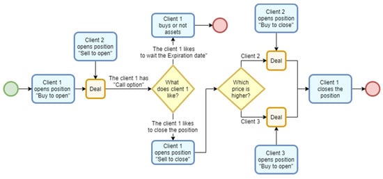
Figure 1.
Stock exchange transaction process with options.
2.2. Betting in iGaming: Approach Without Innovation
In the context of sports betting within iGaming, the fundamental concept is the bet, which represents a transaction between the bookmaker and the client. The client, confident in their ability to predict the outcome of one or more sporting events offered by the bookmaker on the iGaming platform, places a bet by wagering a certain amount, referred to as the stake. After the completion of the final sporting event included in the bet (the settlement date), the bet may be liquid if the client’s predictions are correct. In that case, the bookmaker pays the client a payout, which is inversely proportional to the probability of the event’s occurrence but is known at the moment the bet is placed. If the bet is illiquid, i.e., the prediction does not materialize, the client loses the amount wagered.
Before the settlement date, the bookmaker may offer an early payout option known as “Cash Out”. The client has the right to decide whether to accept the offered cash-out amount—either to realize a small profit if the current situation is favorable, or to minimize potential losses if the situation turns unfavorable. Accepting the cash-out offer closes the bet. Otherwise, the client remains in anticipation of a potentially higher payout at the bet’s settlement date, albeit at a higher level of risk.
The process is illustrated in Figure 2.
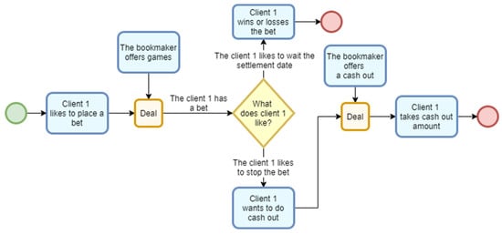
Figure 2.
iGaming sports betting process (approach without innovation).
A clear analogy can be established between options transactions on the stock exchange and a sports bet in iGaming. In both cases, the processes are structurally similar, with the client’s ultimate goal being the realization of profit. The most significant difference between the two mechanisms lies in the absence of an equivalent to the “Buy to open” position in iGaming when a client wishes to close their position through “Sell to close”. Currently, iGaming platforms do not offer the possibility for a client to terminate a bet by selling it to another client who seeks to profit from the same events.
Introducing a functionality that enables the matching of a “Buy to open” order from one client with a “Sell to close” order from another would represent a potential innovation in iGaming. The implementation of the financial derivative “bet buy–sell between two clients” would expand the scope of iGaming. This functionality would allow clients to select the most advantageous price for themselves, while the bookmaker would generate fees from such transactions. Such diversification would lead to a redistribution of capital aimed at reducing financial risk for both clients and the bookmaker.
2.3. Association Between the Bet and the Financial Derivative: Innovation Approach
For the purposes of this study, the term “bet” will be used in a generalized sense, regardless of whether it refers to a single bet or a multiple bet (multi bet) involving one or more games. This unified definition is also applicable to the analogy with the purchase of a call option, as the number of included games is not essential to the mechanisms under consideration.
On the maturity date, the option in iGaming is considered liquid only if all predictions related to the completed games are successful.
The term “unfinished games” refers to sporting events that, at the moment when the “Sell to close” option is initiated by the client holding the bet, are either in progress (live) or yet to start.
The bet, or “call option” in iGaming, possesses the following characteristics:
—Count of games: .
—Odds for game , where .
—Total odds, which—similarly to the fixed strike price of shares—play a role in determining the client’s profit when the option becomes liquid.
S1—Stake amount, or premium (“Premium paid”), which represents the payment made for executing the transaction.
When the maturity date is reached and the call option is liquid, the expected return (“Payout”) from the transaction is
The profit is calculated as
The possibility of early position closure (“Sell to close”) is an essential element of bet management. Once at least one of the events included in the bet has started, the odds associated with the prediction undergo dynamic changes. In response to these fluctuations, the bookmaker may offer a “cash-out” option (“Buy to close”), which represents a form of early settlement of the bet.
A key condition for offering a cash-out is the presence of between one and N unfinished games, while all completed games must be winning ones. This means that, at the moment the transaction is offered, the option must be liquid, i.e., the client is in a profitable position based on the results achieved up to that point.
—Number of unfinished games included in the bet: .
—Total odds of the unfinished games.
—Cash-out amount offered by the bookmaker.
The pricing function that determines the value of bets is confidential information and constitutes a trade secret for each bookmaker. The price of the “Buy to close” order (COA) is set by the bookmaker. In turn, the client independently defines the price of their “Sell to close” order—that is, the minimum price at which they are willing to close their position. The decision on whether the bookmaker’s buyback offer is satisfactory remains entirely at the client’s discretion.
If the “Buy to open” order were to be implemented in iGaming during this intermediate period, a new market participant would emerge—a second client, who wishes to purchase the bet (“call option”) from the first client and thereby open their own position. This second client would determine their own price for the “Buy to open” order.
The overall approach in the included innovation is shown in Figure 3.

Figure 3.
iGaming sports betting process with innovation.
Figure 3.
iGaming sports betting process with innovation.

All transactions would be executed within the bookmaker’s platform, which would collect fees for the completed trades. These fees may include
SF (Sell Fee): A fee paid by the seller to the company (bookmaker).
PF (Purchase Fee): A fee paid by the buyer to the company (bookmaker).
2.4. P2P Models in iGaming: Review of Existing Practices
The proposed innovation represents a specific variant of peer-to-peer (P2P) transactions within the betting sector. An analysis of existing P2P services in the iGaming industry allows for the identification of the following principal models.
2.4.1. Odds Exchange
Under the Odds Exchange model, a user of the platform offers their own odds on the occurrence or non-occurrence of a particular event. Another user may accept these odds and place a bet accordingly. In the event of a winning outcome, the payout is made by the party that offered the odds.
Such platforms do not operate as traditional bookmakers, but rather as intermediaries facilitating a market in which users bet against one another, which in essence constitutes a form of betting position trading, i.e., the buying and selling of risk exposure. The platform operator provides the technical infrastructure and charges a fee or commission for the service. Examples of such platforms include Betfair, Smarkets, Matchbook, Betdaq, and others.
2.4.2. PropSwap-Type P2P Service
The PropSwap platform offers a P2P model for the resale of already placed bets, which may be either physical (paper tickets) or online, and may have been placed with any bookmaker. The seller is the original holder of the bet and offers the associated rights to another participant.
Upon completion of a transaction, physical betting slips are transferred via courier, while online bets are reassigned through a specific procedural mechanism defined by the platform. The platform charges a commission for facilitating the transaction.
At present, this type of P2P service operates under a legal and regulatory framework exclusively within the United States. The service is limited to pre-match bets and is available only prior to the commencement of the first event included in the bet. Although the platform theoretically allows for multiple (parlay) bets, such offers are rarely observed in practice.
An analysis of the platform indicates that the service is utilized by a limited number of sellers who, based on their operational strategies, appear to function primarily as affiliate or marketing partners of bookmakers. Given the relatively low reported annual profit (approximately USD 140,000 for 2024), it may be concluded that this model has not achieved significant market adoption to date.
2.4.3. P2P Service Corresponding to the Proposed Innovation
Within the scope of the present study, no existing P2P service in the iGaming sector was identified that fully corresponds to the model of the proposed innovation. While conceptually comparable to PropSwap-type services, the proposed model differs in several fundamental aspects:
- •
- The service applies to both pre-match and live bets, with pre-match bets being eligible for sale at any point from placement until the conclusion of the final event within the bet.
- •
- There is no requirement for slow physical transfer via courier or complex manual online procedures; the transfer process is fully automated and highly streamlined.
- •
- The bookmaker retains full control over risk exposure, as resale is permitted only during periods in which the bet is eligible for cash-out, thereby preventing the creation of new risk positions or the opening of additional events.
- •
- The secondary market operates within the boundaries of the primary market, with all transactions being bounded, observable, and auditable, thereby enabling global licensing potential and regulatory compliance.
3. Innovation Details
3.1. Minimum Selling Price
A seller holding an open position will not execute a transaction at a price lower than the one offered by the company (bookmaker) for the buyback of the option, i.e., the COA (“Buy to close”) price. This value defines the minimum acceptable selling price for the client. When the selling fee (SF) is added, the minimum selling price can be calculated using the following formula:
At this minimum price, the seller will not achieve a higher profit from the transaction with the “Buy to open” buyer compared to the deal with the bookmaker through the cash-out (“Buy to close”) option. Conversely, the “Buy to open” buyer would realize the maximum profit on the maturity date, provided that the option remains liquid.
3.2. Maximum Selling Price
A client wishing to open a position (“Buy to open”) in order to profit from the unfinished games may purchase a new call option from the bookmaker, who assumes the “Sell to open” position. Given the remaining odds Krest, the expected payout would be equal to Payout1.
The maximum price that the buyer is willing to pay for this option can be defined as
If this is the price the seller is willing to accept, then it makes no difference to them whether they sell the option through a “Buy to close” transaction to another client or purchase a new “Buy to open” option from the bookmaker. In this sense, this represents the maximum price the seller can demand from the buyer. Including the buyer’s fee (PF) and using Equation (7), the maximum selling price is calculated as
At this price, the seller realizes the maximum possible profit, while the buyer does not gain any additional profit from the transaction with the seller; in other words, the buyer’s profit would be the same as if they had purchased the option directly from the bookmaker.
3.3. Optimal Selling Price
The arithmetic calculation of the price, based on the minimum and maximum values, does not guarantee mutual benefit for the seller and the buyer due to the presence of the two transaction fees (SF and PF). The optimal price, (“Sell to close” Price)_Opt, at which both parties realize equal profit from the overall transaction, can be calculated using the following formula:
where
—The amount received by Client 1 in the event of a transaction with another client is equal to the transaction price (for example, the optimal price) minus the Sell Fee (SF).
—The amount paid by Client 1 in the absence of a transaction with another client is equal to the cash-out amount (COA) offered by the bookmaker.
—The amount paid by Client 2 in the absence of a transaction is equal to the stake amount placed with the bookmaker.
—The amount paid by Client 2 in the event of a transaction with another client is equal to the transaction price (for example, the optimal price) plus the Purchase Fee (PF).
After substituting the above-mentioned values into Equation (9) and taking Equation (7) into account, the following expression is obtained after transformation:
If the transaction is executed at the optimal price (PriceOpt), the seller will receive an amount greater than the COA by exactly the same margin that the buyer pays less than they would have to pay the bookmaker for a new bet to achieve the same payout on the maturity date as with the purchased option. In short, at this price, both the buyer and the seller will realize a mutually beneficial transaction.
4. Diversification Model: Scenarios and Phases
For the purpose of constructing and testing the proposed model, it is essential to define all possible scenarios. These scenarios are built upon three basic assumptions and combinations of outcomes across five conditions. Each scenario is characterized by a probability of occurrence (input parameter) and a net profit (positive or negative) for all participating parties (output parameter).
4.1. Basic Statements Applicable to All Scenarios
Statement 1. Client 1 initiates a Buy to open position by acquiring an option from the bookmaker, who takes the Sell to open position. The liquidity of this option directly depends on the outcomes of all N games.
Statement 2. Client 2 initiates a Buy to open position by acquiring an option whose liquidity depends on the outcomes of M games, which constitute a subset of the total N games.
Statement 3. All scenarios proceed through three consecutive phases:
Phase 1—Covers the period from the purchase of the option by Client 1 until the completion of the first (N − M) games.
Phase 2—Encompasses the actions related to Client 1’s decision on whether and to whom to sell their option, as well as the purchase of an option by Client 2.
Phase 3—Covers the period from the start of game (N − M + 1) until the completion of game number N (the final game).
4.2. Scenarios: Participants, Input and Output Parameters
Option 1 is defined as the option purchased by Client 1 from the bookmaker. Option 2 is the option purchased by Client 2 from the bookmaker. Under the condition of liquidity at the end of Phase 3, both options generate an identical payout—this is the fundamental assumption on which the present study is based.
The dependencies regarding the liquidity of the options are presented in Table 1.

Table 1.
Dependencies regarding the liquidity of the options.
The scenarios to be analyzed are formed based on the outcomes of the following five conditions. A summarized representation of these scenarios is provided in Figure 4.
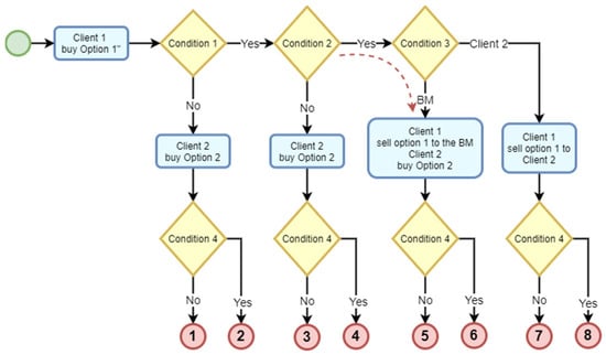
Figure 4.
A summarized representation of the scenarios.
Condition 1. Is Option 1 liquid or not after Phase 1? (Do the first N − M games win or lose?)
Condition 2. Does Client 1 want to sell Option 1 or not?
Condition 3. To whom does Client 1 wish to sell their option? (Take cash out or sell the bet?)
Condition 4. Is Option 2 liquid or not on the maturity date? (Do the last M games win or lose?)
All possible scenarios are summarized in Table 2. The combinations of the outcomes of the conditions that define the scenarios are presented.
Table 2.
All possible scenarios.
denotes the profit of Player 1 under Outcome i.
denotes the profit of Player 2 under Outcome i.
denotes the profit of the bookmaker under Outcome i.
For each outcome, the formulas for the profits of Player 1 and Player 2 are provided. The formula for the bookmaker is identical across all outcomes and is as follows:
Exit 1
At the end of Phase 1, Option 1 held by Player 1 is illiquid, and they lose their premium.
During Phase 2, Player 2 purchases Option 2, and at the end of Phase 3 it becomes illiquid, resulting in the loss of their premium.
Exit 2
At the end of Phase 1, Option 1 held by Player 1 is illiquid, and they lose their premium.
During Phase 2, Player 2 purchases Option 2, and at the end of Phase 3 it becomes liquid, resulting in a profit for them.
Exit 3
Option 1 is liquid at the end of Phase 1, but Player 1 chooses not to sell it before the maturity date. They hold it until the end of Phase 3, when it becomes illiquid, resulting in the loss of their premium.
During Phase 2, Player 2 purchases Option 2, and at the end of Phase 3 it is illiquid, resulting in the loss of their premium.
Exit 4
Player 1 does not sell Option 1 before the maturity date. They hold it until the end of Phase 3, when it becomes liquid, resulting in a profit.
Player 2 purchases Option 2, and at the end of Phase 3 it becomes liquid, resulting in a profit.
Exit 5
Player 1 wishes to realize an early profit from Option 1 and sells it to Player 3 at the COA price. Player 2 then purchases Option 2 from Player 3, and it becomes illiquid on the maturity date.
Exit 6
Player 1 sells Option 1 to Player 3, while Player 2 earns a profit from Option 2.
Exit 7
Player 1 wishes to realize an early profit from Option 1 and sells it to Player 2. Option 1 becomes illiquid on the maturity date. It is assumed that the transaction between Player 1 and Player 2 takes place at a mutually beneficial price.
Exit 8
Player 1 sells Option 1 to Player 2, and it becomes liquid on the maturity date.
On a global scale, iGaming represents an extremely profitable sector of the economy, which implies that, in aggregate terms, clients function as net losers, while profits are realized by a limited number of individual participants. In this context, any innovation within the system could be perceived positively by all parties, provided that it increases profitability for clients (Player 1 and Player 2) or at least does not generate greater losses for them, while the bookmaker’s costs remain within acceptable limits relative to the expected benefits. Potential benefits include an increase in the number of newly registered users attracted by the innovation, as well as the strengthening of the bookmaker’s corporate image as a technologically oriented and innovative company.
To examine the effect of the proposed innovation on the profits of all participants, a simulation will be carried out using the Python 3.9.7 programming environment. For analytical purposes, a comparative approach will be applied, evaluating the financial outcomes under two scenarios—without the innovation and with the innovation implemented. In the simulation model corresponding to the second scenario, the workflow illustrated in Figure 4 will be used. In the absence of the innovation, Condition 3 will not apply, and the outcome “Yes” from Condition 2 will lead directly to Condition 4, as indicated by the red dashed connection shown in Figure 4.
After analyzing Formulas (11)–(27), it can be summarized that the probabilities and profits of the players in all examined scenarios are determined by three variable parameters (), two constant parameters (SF%, PF%), and two variable probabilities: the probability that a player will sell their option before the maturity date () and, in the event of a sale, the choice of counterparty—either another player () or the bookmaker ().
The remaining probabilities, including () and (), are functions of the total odds (), the residual odds (), the margin, the total number of games, and the number of games not yet started during Phase 1. The COA parameter formally appears in the analytical expressions but can essentially be regarded as a function—albeit with an unknown analytical form—of the aforementioned variable parameters.
The probability () directly depends on the probabilities of the predictions for the games within the subset N−M, that is, those concluding by the end of Phase 1. Assuming that the odds are not subject to manipulation [12] and that the margin is homogeneous across all games, the probability () can be expressed as follows:
The probability is determined by a variety of specific factors, including—but not limited to—the sociocultural characteristics of the players, their individual behavioral profiles, and their level of risk tolerance. Within the iGaming sector, the average share of participants who tend to close their bets before their natural completion reaches approximately 50%. Therefore, it can be assumed that .
In turn, the probability is currently empirically undefined, as the functionality described in this study represents an innovation that has not yet been subjected to market testing. Due to the lack of empirical data on the degree of player adoption, a tentative assumption can be made that its initial use will be conservative—for example, around . As a result of an effective marketing strategy and communication campaign, this share could increase to around 50% or more for bets placed before the start of sporting events. In contrast, the limited reaction time typical of live games is likely to reduce the applicability of the new functionality in that segment. In general terms, it can be assumed that .
As for the probabilities , they are determined by the forecast probabilities calculated by Player 2 for all M considered games, representing a derivative function of the individual accuracy of their predictions.
Solely for the purposes of the simulation, it is assumed that .
For each iteration, given a combination of the values of and , the variable parameters will take random values within the following ranges:
, where and are defined by the bookmaker. For testing purposes, .
In practice, the distribution of is not linear within the specified range. The frequency is highest at the lower values and lowest at the higher ones. For testing purposes, can take values according to the following formula:
The value of r will be generated by a random number generator (RNG) within the range [0 ÷ 1].
By analogy, the value of KTotal will be determined within the range . The minimum and maximum values are set based on the author’s experience in the field of iGaming.
For , it is assumed that it follows a linear distribution within the following range: .
A total of 1000 iterations are performed for each combination of and values. The simulations were performed using the code in Appendix A. The results are presented in Figure 5, Figure 6 and Figure 7.
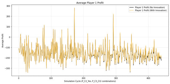
Figure 5.
Average profit for player 1.
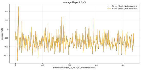
Figure 6.
Average profit for player 2.
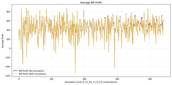
Figure 7.
Average profit for player 3.
As a result of the simulations conducted, an increase in the profits of Player 1 and Player 2 is observed. For Player 1, the gain ranges from 0.5% to 1.5%, while for Player 2 the variation is between 0.5% and 1.0%. Player 1’s profit arises from the fact that when they decide to sell their bet and enter into a transaction with Player 2, they receive a higher amount for their bet than the cash-out value. Player 2’s profit results from the fact that when placing a bet, they pay a lower price if they conclude a deal with Player 1 than if they purchase it from the bookmaker.
On the betting platform, cash inflows come from customers’ bets. These amounts are redistributed between winning customers and the bookmaker. Since Player 1 and Player 2 both make a profit, this occurs at the bookmaker’s expense. Partial compensation for the reduced revenues comes from the fees charged for the selling and buying of bets between Player 1 and Player 2. The simulation shows that the bookmaker records a reduction in profit on the order of 1–1.5%. This is the cost the bookmaker pays for introducing the innovation. In practice, these 1–1.5% coincide exactly with the percentages that bookmakers typically spend on promotions and the deployment of new innovations.
Graphically, these relationships are illustrated in Figure 5 and Figure 6, where the increase in players’ profits is represented by black peaks corresponding to portions of the negative peaks of the functions. For the bookmaker (Player 3), the analogous black peaks in Figure 7 appear at the positive peaks, reflecting the decrease in profit and confirming the opposite dynamics of their results compared to those of the participants.
5. Conclusions
It should be emphasized that the proposed model has certain limitations. All parameter distributions used in the model are derived from empirical practice; however, this practice is associated with a specific bookmaker and a specific market. Consequently, when the model is applied in a different geographical context, country, or market, customer behavior may differ.
The probability of early bet termination depends on multiple factors, some of which cannot be directly observed or quantitatively measured. For this reason, the applied percentage represents an averaged hypothetical value. Similarly, the proportion of early terminations that remain linked to the cash-out mechanism and the proportion that may be redirected to the proposed innovation are also hypothetical quantities. As a result, the conclusions drawn from the simulation exhibit a probabilistic nature and should be interpreted with due caution.
Despite the limitations of the assumptions, the results of the simulation indicate that the proposed innovation has a positive effect on the profitability of both players. This finding suggests a high likelihood that the innovation would be favorably received by participants in the iGaming sector. The introduction of the “Sell to close” option, in synergy with “Buy to open”, could attract significant interest among players by serving as a mechanism for optimizing their trading strategies. Such functionality could contribute to the diversification of the gaming portfolio, simultaneously enhancing market participants’ security and expanding their opportunities for achieving higher returns.
At present, there is no established legal or regulatory framework applicable to P2P transactions of the type proposed by the innovation due to the fact that such transactions have not yet been introduced or implemented in practice. It is expected that the relevant regulatory regime will be formulated ex post, once the competent regulatory authority has had the opportunity to assess a functioning product or market model in operation.
The transparent nature of the transaction under consideration, the mechanisms designed to prevent the emergence of an unregulated (“wild”) market, and the existence of a reference pricing framework defined by the value of the cash-out mechanism, create the necessary conditions for the relatively smooth and coherent establishment of an appropriate legal and regulatory framework for the respective innovation.
As expected, the implementation of this innovation negatively affects the bookmaker’s revenues, which may be viewed as an inevitable cost of market adaptation and technological advancement. Nevertheless, it is likely that the innovation will stimulate an expansion of the customer base within the iGaming industry, attracting new users motivated both by the potential for higher profits and by an interest in new yet effective market solutions.
Author Contributions
Conceptualization, P.I. and D.O.; methodology, P.I.; software, P.I.; validation, D.O.; formal analysis, P.I. and D.O.; investigation, D.O.; resources, P.I.; data curation, P.I.; writing—original draft preparation, P.I.; writing—review and editing, D.O.; visualization, P.I.; supervision, P.I. and D.O.; project administration, P.I. and D.O.; funding acquisition, D.O. All authors have read and agreed to the published version of the manuscript.
Funding
This research was funded by frames of Bulgarian National Recovery and Resilience Plan, Component “Innovative Bulgaria”, the Project Nº BG-RRP-2.004-0006-C02 “Development of research and innovation at Trakia University in service of health and sustainable well-being”.
Institutional Review Board Statement
Not applicable.
Informed Consent Statement
Not applicable.
Data Availability Statement
The original contributions presented in this study are included in the article. Further inquiries can be directed to the corresponding author.
Conflicts of Interest
The authors declare no conflicts of interest.
Abbreviations
The following abbreviations are used in this manuscript:
| COA | Cash Out Amount |
| SF | Sell Fee |
| PF | Purchase Fee |
Appendix A
import pandas as pd
import numpy as np
import random
import matplotlib.pyplot as plt
# --- 1. Defining constants and functions ---
# Fee
SF = 0.05 # 5% Sellary fee
PF = 0.05 # 5% Purchase fee
# COA calculation
def calculate_coa(stake_1, k_total, k_rest):
return stake_1 * (k_total / k_rest) * (0.4 + 4 / (k_rest + 8))
# Optimal price
def calculate_price_opt(stake_1, k_total, k_rest, coa, sf, pf):
return ((stake_1 * k_total) / k_rest + coa)/(2 + pf - sf)
# --- 2.Profit definition for each exit for each player ---
# Exit 1
def profit_p1_e1(stake_1): return -stake_1
def profit_p2_e1(stake_1, k_total, k_rest): return -stake_1 * k_total / k_rest
# Exit 2
def profit_p1_e2(stake_1): return -stake_1
def profit_p2_e2(stake_1, k_total, k_rest): return ((stake_1 * k_total) / k_rest) * (k_rest - 1)
# Exit 3
def profit_p1_e3(stake_1): return -stake_1
def profit_p2_e3(stake_1, k_total, k_rest): return -stake_1 * k_total / k_rest
# Exit 4
def profit_p1_e4(stake_1, k_total): return stake_1 * (k_total - 1)
def profit_p2_e4(stake_1, k_total, k_rest): return stake_1 * k_total / k_rest * (k_rest - 1)
# Exit 5
def profit_p1_e5(stake_1, coa): return coa - stake_1
def profit_p2_e5(stake_1, k_total, k_rest): return -stake_1 * k_total / k_rest
# Exit 6
def profit_p1_e6(stake_1, coa): return coa - stake_1
def profit_p2_e6(stake_1, k_total, k_rest): return stake_1 * k_total * (1 - 1 / k_rest)
# Exit 7
def profit_p1_e7(stake_1, price_opt, sf): return price_opt * (1 - sf) - stake_1
def profit_p2_e7(price_opt, pf): return -price_opt * (1 + pf)
# Exit 8
def profit_p1_e8(stake_1, price_opt, sf, k_total): return price_opt * (1 - sf) - stake_1
def profit_p2_e8(stake_1, k_total, price_opt, pf): return stake_1 * k_total - price_opt * (1 + pf)
# --- 3. Parameters of the simulation ---
num_iterations = 1000 # Number of simulations for each loop
# P_C2_Yes scope & P_C3_Cl2 scope
p_c2_yes_range = np.arange(0, 0.61, 0.03) # Probability Player 1 to sell Option 1
p_c3_cl2_range = np.arange(0, 0.61, 0.03) # Probability Player 1 to sell Option 1 to Player 2
# --- 4. RNG Function ---
def probability_generator():
max_odds_count = 50
min_odds = 1.05
max_odds = 2.20
margin = 0.05
min_stake = 10
max_stake = 10000
max_K_total = 100
found = False
while not found:
# RNG: Stake
stake = np.exp(random.uniform(np.log(min_stake), np.log(max_stake)))
# RNG: Count of games (The total count & The rest count)
N = int(np.exp(random.uniform(np.log(2), np.log(max_odds_count))))
M = int(random.uniform(1, N - 1))
# RNG: A list of N odds
odds_list = np.exp(np.random.uniform(np.log(min_odds), np.log(max_odds), N))
# Calculating: K total
K_total1 = np.prod(odds_list)
# Calculating: K rest
K_rest1 = np.prod(odds_list[(N - M):])
if (K_total1 < max_K_total) & (stake * K_total1 / K_rest1 < max_stake):
found = True
# Calculating: Probability to win N games, The last (N-M+1) games, the first (N-M) games
P_M = 1 / (K_rest1 * (1 + margin)**(N - M + 1))
P_N_M = 1 / ((K_total1 / K_rest1) * (1 + margin)**(N - M))
return stake, K_total1, K_rest1, P_M, P_N_M
# --- 5. Main simulation -------------------------------------------------
results_no_innovation = [] # To preserve average profits without innovation
results_with_innovation = [] # To preserve average profits with innovation
for p_c2_yes_val in p_c2_yes_range:
for p_c3_cl2_val in p_c3_cl2_range:
# Totals for winnings for the current cycle
total_profit_p1_no_inn = 0
total_profit_p2_no_inn = 0
total_profit_p1_with_inn = 0
total_profit_p2_with_inn = 0
for _ in range(num_iterations):
stake1, K_total1, K_rest, P_M, P_N_M = probability_generator()
stake_1 = stake1
k_total = K_total1
k_rest = K_rest
p_c1_yes_game = P_N_M # Probability of Option 1 being liquid after Phase 1
p_c4_yes_game = P_M # Probability of Option 2 being liquid after Phase 3
# COA и Price_Opt calculations
coa = calculate_coa(stake_1, k_total, k_rest)
price_opt = calculate_price_opt(stake_1, k_total, k_rest, coa, SF, PF)
# Generation of probability for each condition
p1 = random.random()
p2 = random.random()
p3 = random.random()
p4 = random.random()
# Profit initialisation
current_profit_p1_no_inn = 0
current_profit_p2_no_inn = 0
current_profit_p3_no_inn = 0
# ========================================
# === Simulation WITHOUT the inovation ===
# ========================================
if p1 < p_c1_yes_game: # Condition 1
# C1_yes (Bet 1 is alive)
if p2 < p_c2_yes_val: # Condition 2
# C1_Yes -> C2_Yes (Player 1 make cash out, Player 2 place a bet 2)
if p4 < p_c4_yes_game: # Condition 5
# Exit 6 | C1_Yes -> C2_Yes -> C5_Yes (Bet 1 is cashed out, Bet 2 is won)
current_profit_p1_no_inn = profit_p1_e6(stake_1, coa)
current_profit_p2_no_inn = profit_p2_e6(stake_1, k_total, k_rest)
else: # Exit 5 | C1_Yes -> C2_Yes -> C5_No (Bet 1 is cashed out, Bet 2 is lost)
current_profit_p1_no_inn = profit_p1_e5(stake_1, coa)
current_profit_p2_no_inn = profit_p2_e5(stake_1, k_total, k_rest)
else: # C1_Yes -> C2_No (The Payer 1 doesn't sell)
if p4 < p_c4_yes_game: # Condition 5:
# Exit 4 | C1_Yes -> C2_No -> C4_Yes (Bet 1 is won, Bet 2 is Won)
current_profit_p1_no_inn = profit_p1_e4(stake_1, k_total)
current_profit_p2_no_inn = profit_p2_e4(stake_1, k_total, k_rest)
else: # Exit 3 | C1_Yes -> C2_No -> C4_No (Bet 1 is lost, Bet 2 is lost)
current_profit_p1_no_inn = profit_p1_e3(stake_1)
current_profit_p2_no_inn = profit_p2_e3(stake_1, k_total, k_rest)
else: # C1_No
if p4 < p_c4_yes_game: # Condition 5:
# Exit 2 | C1_No -> C5_Yes
current_profit_p1_no_inn = profit_p1_e2(stake_1)
current_profit_p2_no_inn = profit_p2_e2(stake_1, k_total, k_rest)
else: # Exit 1 | C1_No -> C5_No
current_profit_p1_no_inn = profit_p1_e1(stake_1)
current_profit_p2_no_inn = profit_p2_e1(stake_1, k_total, k_rest)
total_profit_p1_no_inn += current_profit_p1_no_inn
total_profit_p2_no_inn += current_profit_p2_no_inn
# ======================================
# === Simulation WITH the inovation ===
# ======================================
current_profit_p1_with_inn = 0
current_profit_p2_with_inn = 0
current_profit_p3_with_inn = 0
if p1 < p_c1_yes_game: # Condition 1:
# C1_Yes (Bet 1 is alive)
if p2 < p_c2_yes_val: # Condition 2
# C1_Yes -> C2_Yes (Player 1 wants to sell Bet 1)
if p3 < p_c3_cl2_val: # Condition 3
# C1_Yes -> C2_Yes -> C3_Client2 (Player 1 sells Bet 1 to Player 2)
if p4 < p_c4_yes_game: # Condition 5:
# Exit 8 | C1_Yes -> C2_Yes -> C3_Client2 -> C4_Yes (Bet 1 is won)
current_profit_p1_with_inn = profit_p1_e8(stake_1, price_opt, SF, k_total)
current_profit_p2_with_inn = profit_p2_e8(stake_1, k_total, price_opt, PF)
else: # Exit 7 | C1_Yes -> C2_Yes -> C3_Client2 -> C4_No (Bet 1 is lost)
current_profit_p1_with_inn = profit_p1_e7(stake_1, price_opt, SF)
current_profit_p2_with_inn = profit_p2_e7(price_opt, PF)
else: # C1_Yes -> C2_Yes -> C3_Bookmaker (Player 1 maked cash out, Player 2 place Bet 2)
if p4 < p_c4_yes_game: # Condition 5:
# Exit 6 | C1_Yes -> C2_Yes -> C3_Bookmaker -> C5_Yes (Bet 1 is cashed out, Bet 2 is Won)
current_profit_p1_with_inn = profit_p1_e6(stake_1, coa)
current_profit_p2_with_inn = profit_p2_e6(stake_1, k_total, k_rest)
else: # Exit 5 | C1_Yes -> C2_Yes -> C3_Bookmaker -> C5_No(Bet 1 is cashed out, Bet 2 is Lost)
current_profit_p1_with_inn = profit_p1_e5(stake_1, coa)
current_profit_p2_with_inn = profit_p2_e5(stake_1, k_total, k_rest)
else: # 1_Yes -> C2_No (Player 1 doesn't wants to sell Bet 1, Player 2 place a Bet 2)
if p4 < p_c4_yes_game: # Condition 5:
# Exit 4 | 1_Yes -> C2_No -> C4_Yes (Bet 1 is won, Bet 2 is won)
current_profit_p1_with_inn = profit_p1_e4(stake_1, k_total)
current_profit_p2_with_inn = profit_p2_e4(stake_1, k_total, k_rest)
else: # Exit 3 | 1_Yes -> C2_No -> C4_No (Bet 1 is lost, Bet 2 is lost)
current_profit_p1_with_inn = profit_p1_e3(stake_1)
current_profit_p2_with_inn = profit_p2_e3(stake_1, k_total, k_rest)
else: # C1_No (Bet 1 is lost)
if p4 < p_c4_yes_game: # Condition 5: Опция 2 ликвидна ли е на падежа?
# Exit 2 | {Bet 1 is lost, Bet 2 is won}
current_profit_p1_with_inn = profit_p1_e2(stake_1)
current_profit_p2_with_inn = profit_p2_e2(stake_1, k_total, k_rest)
else: # Exit 1 | {Bet 1 is lost, Bet 2 is lost}
current_profit_p1_with_inn = profit_p1_e1(stake_1)
current_profit_p2_with_inn = profit_p2_e1(stake_1, k_total, k_rest)
total_profit_p1_with_inn += current_profit_p1_with_inn
total_profit_p2_with_inn += current_profit_p2_with_inn
# Bookmaker's profit = - (Player 1 profit + Player 2 profit)
total_profit_p3_no_inn = -(total_profit_p1_no_inn + total_profit_p2_no_inn)
total_profit_p3_with_inn = -(total_profit_p1_with_inn + total_profit_p2_with_inn)
# Storing average profits for the current cycle
results_no_innovation.append({
'P_C2_Yes': p_c2_yes_val,
'P_C3_Cl2': p_c3_cl2_val,
'Avg_P1_Profit': total_profit_p1_no_inn / num_iterations,
'Avg_P2_Profit': total_profit_p2_no_inn / num_iterations,
'Avg_P3_Profit': total_profit_p3_no_inn / num_iterations
})
results_with_innovation.append({
'P_C2_Yes': p_c2_yes_val,
'P_C3_Cl2': p_c3_cl2_val,
'Avg_P1_Profit': total_profit_p1_with_inn / num_iterations,
'Avg_P2_Profit': total_profit_p2_with_inn / num_iterations,
'Avg_P3_Profit': total_profit_p3_with_inn / num_iterations
})
# Total results_no_innovation
sum_p1_no = sum(item['Avg_P1_Profit'] for item in results_no_innovation)
sum_p2_no = sum(item['Avg_P2_Profit'] for item in results_no_innovation)
sum_p3_no = sum(item['Avg_P3_Profit'] for item in results_no_innovation)
# Total results_with_innovation
sum_p1_with = sum(item['Avg_P1_Profit'] for item in results_with_innovation)
sum_p2_with = sum(item['Avg_P2_Profit'] for item in results_with_innovation)
sum_p3_with = sum(item['Avg_P3_Profit'] for item in results_with_innovation)
# Profit comparing
print(f"Player 1, Avg Profit, Without inovation = {round(sum_p1_no,0)}")
print(f"Player 1, Avg Profit, With inovation = {round(sum_p1_with,0)}")
print("Diferences: Avg Profit, With inovation - Avg Profit, Without inovation =",round(sum_p1_with - sum_p1_no,0))
print("Diferences / Avg Profit, Without inovation =",round(-(sum_p1_with - sum_p1_no) / sum_p1_no,4)*100, "%")
print("----------------------------------------------------------------")
print(f"Player 2, Avg Profit, Without inovation = {round(sum_p2_no,0)}")
print(f"Player 2, Avg Profit, With inovation = {round(sum_p2_with,0)}")
print("Diferences: Avg Profit, With inovation - Avg Profit, Without inovation =",round(sum_p2_with - sum_p2_no,0))
print("Diferences / Avg Profit, Without inovation =",round(-(sum_p2_with - sum_p2_no) / sum_p2_no,4)*100, "%")
print("----------------------------------------------------------------")
print(f"Bookmaker, Avg Profit, Without inovation = {round(sum_p3_no,0)}")
print(f"Bookmaker, Avg Profit, With inovation = {round(sum_p3_with,0)}")
print("Diferences: Avg Profit, With inovation - Avg Profit, Without inovation =",round(sum_p3_with - sum_p3_no,0))
print("Diferences / Avg Profit, Without inovation =",round(-(sum_p3_with - sum_p3_no) / sum_p3_no,4)*100, "%")
print("----------------------------------------------------------------")
#--- 6. Visualization of results ---
p1_profits_no_inn = [r['Avg_P1_Profit'] for r in results_no_innovation]
p1_profits_with_inn = [r['Avg_P1_Profit'] for r in results_with_innovation]
p2_profits_no_inn = [r['Avg_P2_Profit'] for r in results_no_innovation]
p2_profits_with_inn = [r['Avg_P2_Profit'] for r in results_with_innovation]
p3_profits_no_inn = [r['Avg_P3_Profit'] for r in results_no_innovation]
p3_profits_with_inn = [r['Avg_P3_Profit'] for r in results_with_innovation]
# Function about Plotting profits
def show_chart(player, no_inn, with_inn):
plt.figure(figsize=(12, 6))
plt.plot(
no_inn,
label=f'{player} Profit (No Innovation)',
color='black'
)
plt.plot(
with_inn,
label=f'{player} Profit (With Innovation)',
color=(251/255, 199/255, 83/255)
)
plt.title(f'Average {player} Profit')
plt.xlabel('Simulation Cycle (P_C2_Yes, P_C3_Cl2 combinations)')
plt.ylabel('Average Profit')
plt.grid(True, alpha=0.3)
plt.legend()
plt.tight_layout()
plt.show()
return
# visualisation
sh = show_chart ("Player 1", p1_profits_no_inn, p1_profits_with_inn)
sh = show_chart ("Player 2", p2_profits_no_inn, p2_profits_with_inn)
sh = show_chart ("BM", p3_profits_no_inn, p3_profits_with_inn)
References
- Statistical Classification of Economic Activities in the European Community, p. 89. Available online: https://stat.gov.pl/files/gfx/portalinformacyjny/en/defaultstronaopisowa/3249/1/1/poz_nace_rev2.pdf?utm_source=chatgpt.com (accessed on 22 September 2025).
- Penttinen, E.; Halme, M.; Malo, P.; Saarinen, T. Playing for fun or for profit: How extrinsically-motivated and intrinsically-motivated players make the choice between competing dual-purposed gaming platforms. Electron. Mark. 2018, 29, 337–358. [Google Scholar] [CrossRef]
- Rabinovitz, S.; Packin, N.G. All Bets Are On: Addiction, Prediction, Regulation, and the Future of Financial Gambling. Fordham Intellect. Prop. Media Entertain. Law J. 2025, 36, 90. [Google Scholar]
- What Is Arbitrage?, StoneX. Available online: https://www.stonex.com/en/financial-glossary/arbitrage/ (accessed on 8 October 2025).
- Sinclair, E.S.-L.L.; Clark, L.; Wohl, M.J.A.; Keough, M.T.; Kim, H.S. Cash outs during in-play sports betting: Who, why, and what it reveals. Addict. Behav. 2024, 154, 108008. [Google Scholar] [CrossRef] [PubMed]
- Hedging with Betfair. Available online: https://www.aussportsbetting.com/guide/other-topics/hedging-with-betfair/ (accessed on 16 September 2025).
- Chen, J. What Does “Buy to Open” Mean in Options Trading? A Comprehensive Guide, 2025. Available online: https://www.investopedia.com/terms/b/buytoopen.asp (accessed on 18 November 2025).
- Chen, J. Sell to Open: How It Works in Options Trading with Examples, 2025. Available online: https://www.investopedia.com/terms/s/selltoopen.asp (accessed on 18 November 2025).
- Fernando, J. Call Option: What It Is, How to Use It, and Examples, 2025. Available online: https://www.investopedia.com/terms/c/calloption.asp (accessed on 18 November 2025).
- Fernando, J. Understanding Option Strike Prices: Definition, Function, and Impact, 2025. Available online: https://www.investopedia.com/terms/s/strikeprice.asp (accessed on 15 August 2025).
- Chen, J. Understanding Sell to Close in Options Trading: Definition and Examples, 2025. Available online: https://www.investopedia.com/terms/s/selltoclose.asp (accessed on 18 November 2025).
- Iliev, P.; Todorov, D. The Chance or the Margin Drives Bookies’ Revenue. In Proceedings of the MIPRO 48th ICT and Electronics Convention, Opatija, Croatia, 2–6 June 2025; pp. 1013–1019. Available online: https://ieeexplore.ieee.org/xpl/conhome/11131682/proceeding?sortType=vol-only-seq&isnumber=11131702&searchWithin=iliev (accessed on 10 October 2025).


Disclaimer/Publisher’s Note: The statements, opinions and data contained in all publications are solely those of the individual author(s) and contributor(s) and not of MDPI and/or the editor(s). MDPI and/or the editor(s) disclaim responsibility for any injury to people or property resulting from any ideas, methods, instructions or products referred to in the content. |
© 2026 by the authors. Licensee MDPI, Basel, Switzerland. This article is an open access article distributed under the terms and conditions of the Creative Commons Attribution (CC BY) license.