Method for Generating Pseudo-NDVI from RVI Derived from Satellite-Borne SAR Imagery Data Using CycleGAN and pix2pix Models

Abstract

Continuous vegetation monitoring is essential for predicting crop varieties and yields; however, optical satellite data are frequently unavailable due to cloud cover. To overcome this limitation, this study proposes a method for generating pseudo-NDVI (Normalized Difference Vegetation Index) imagery from RVI (Radar Vegetation Index) derived from Synthetic Aperture Radar (SAR) data using Generative Adversarial Networks (GANs). Two architectures—pix2pixHD (supervised) and CycleGAN (unsupervised)—were evaluated using Sentinel-1 and Sentinel-2 data under identical conditions. By introducing RVI as an intermediate feature instead of directly converting SAR backscatter to NDVI, the proposed method enhanced physical interpretability and improved correlation with NDVI. Quantitative results show that pix2pix achieved higher accuracy (SSIM = 0.5667, PSNR = 22.24 dB, RMSE = 20.54) than CycleGAN (SSIM = 0.5240, PSNR = 19.54 dB, RMSE = 28.02), with further improvement when combining VV and VH polarization data. Although the absolute accuracy remains moderate, this approach enables continuous annual NDVI time series reconstruction for crop monitoring under persistent cloud conditions, demonstrating clear advantages over conventional direct SAR-to-NDVI conversion methods.

1. Introduction

Climate change has intensified the frequency and severity of extreme weather events, posing significant risks to global food production and agricultural sustainability. Real-time and scalable crop monitoring has therefore become indispensable for assessing crop conditions, detecting stress early, and optimizing management decisions (FAO, 2021 [1]; Lobell et al., 2020 [2]). Traditional techniques, however, rely predominantly on optical satellite indices, which face substantial operational limitations under persistent cloud cover and adverse weather conditions. For instance, studies have shown that up to 60% of optical satellite observations in tropical and monsoon regions are obscured by clouds during critical growth stages (Zhang et al., 2019), creating data gaps that hinder timely crop assessment [3].

The Normalized Difference Vegetation Index (NDVI), derived from optical multispectral imagery, remains the most widely used index for monitoring vegetation health and photosynthetic capability (Tucker, 1979 [4]; Pettorelli et al., 2005 [5]). NDVI’s effectiveness arises from the strong contrast between red and near-infrared reflectance, which corresponds to chlorophyll content and plant vigor. Yet, because NDVI relies on optical sensors, data availability is severely affected by cloud cover and solar illumination (Huete et al., 2002 [6]). To address these gaps, all-weather radar observations have recently been explored as an alternative or complementary source of vegetation information.

Synthetic Aperture Radar (SAR) provides high spatial and temporal coverage independent of weather or sunlight, making it particularly useful in cloudy environments (Lucas et al., 2012 [7]). The Radar Vegetation Index (RVI), computed from multi-polarized SAR backscatter, has been introduced to quantify vegetation structure and biomass (Kim & van Zyl, 2001 [8]). RVI is sensitive to canopy geometry, surface roughness, and water content, but unlike NDVI, it responds more to vegetation structure than to photosynthetic activity. This structural sensitivity means that while RVI offers robustness under cloudy conditions, it cannot directly replace NDVI in capturing physiological plant parameters (Veloso et al., 2017 [9]).

Recent research has attempted to bridge this gap by learning nonlinear mappings between radar-based features and NDVI through machine learning and generative models. For example, Ayari et al. (2024) [10] reconstructed NDVI time series of wheat fields in Tunisia from Sentinel-1 SAR data using Support Vector Regression (SVR) and Random Forests, demonstrating moderate correlation. Similarly, several studies have explored deep generative models such as CycleGANs and pix2pix for pseudo-NDVI estimation from VH or VV polarization data (Arun Balazji et al., 2023 [11]; Li et al., 2022 [12]). However, their performance remains limited due to the weak and nonlinear relationship between single polarization backscatter coefficients and optical reflectance values.

This study proposes a new approach that employs the RVI as an intermediate physical feature for NDVI generation from SAR data. Because RVI aggregates polarization information and captures vegetation structural properties more comprehensively, it is expected to correlate more strongly with NDVI than raw VH or VV backscatter. Using Generative Adversarial Networks (GANs), particularly pix2pix (paired training) and CycleGAN (unpaired training), this study investigates the conversion of RVI to pseudo-NDVI. The objective is to generate continuous, high-quality NDVI products even under persistent cloud cover, thereby enabling near-real-time crop monitoring, temporal gap-filling in NDVI time series, and improvement in yield estimation accuracy.

2. Related Studies

GANs have recently been explored as powerful tools for synthesizing optical vegetation indices from SAR observations. Early studies demonstrated that GANs, particularly CycleGAN and pix2pix architectures, can generate NDVI-like simulation images from Sentinel-1 C-SAR data, achieving notable performance for specific crops such as beetroot during their active growth stages (e.g., [13]). These approaches were motivated by the increasing need for reliable vegetation indicators in cloud-covered regions, where optical data are often unavailable (https://pmc.ncbi.nlm.nih.gov/articles/PMC9246746/, accessed on 27 December 2025).

In parallel, numerous studies have proposed crop yield estimation models using NDVI derived from optical sensors such as Sentinel-2. By leveraging NDVI time series features, these models achieved prediction accuracies exceeding 90% for crops such as corn and soybeans [14]. Building upon such advancements, more recent research has focused on fusing SAR and optical data to improve temporal consistency and cloud tolerance. SAR’s all-weather imaging capability has proven especially valuable for cloud-gap filling and defect completion in optical datasets (https://pmc.ncbi.nlm.nih.gov/articles/PMC9657195/, accessed on 27 December 2025) [15].

Beyond conventional NDVI reconstruction, several GAN-based methodologies have been developed for pseudo-NDVI generation and SAR-to-optical image translation. For instance, conditional GANs (cGAN) have been employed to synthesize multi-spectral optical images from SAR inputs, thereby mitigating cloud-induced data losses [16]. These SAR-driven generative frameworks have laid the foundation for subsequent research into cloud removal and optical image restoration. Notably, approaches combining Sentinel-1 SAR and Sentinel-2 optical data via GANs demonstrated effective cloud inpainting capabilities, recovering detailed spectral information in occluded regions [17]. Related deep learning frameworks, including ResNet-based SAR–optical fusion architectures, have further improved the robustness of cloud removal processes, particularly under dense cloud conditions (https://pmc.ncbi.nlm.nih.gov/articles/PMC12591094/, accessed on 27 December 2025) [18].

Complementary to direct image conversion, research on estimating vegetation indices from polarimetric SAR has also advanced. Full- and dual-polarization indices such as the RVI and Dual-Pol Radar Vegetation Index (DpRVI) have shown strong sensitivity to vegetation structure and scattering mechanisms [19]. These indices have proven effective for identifying crop growth stages and canopy dynamics, as confirmed through sensitivity analyses of SAR parameters with respect to crop height and canopy coverage [19]. Subsequent studies have utilized Sentinel-1 data to derive cloud-independent NDVI proxies (NDVInc), demonstrating the feasibility of reliable vegetation monitoring purely from radar observations (https://www.jait.us/articles/2025/JAIT-V16N1-37.pdf, accessed on 27 December 2025) [20,21].

Furthermore, advances in high-resolution SAR-to-optical translation have expanded the application scope of GANs. Modified pix2pixHD architectures with spatial attention modules have been successfully applied to enhance spatial resolution and detect landslide-affected areas [22,23]. These methods, occasionally supported by RVI-based change detection, provide promising results for mapping transitions from vegetated to bare-soil conditions (https://www.nature.com/articles/s41598-020-60520-6, accessed on 27 December 2025) [24].

Despite these achievements, most prior studies have attempted direct conversion from SAR backscatter coefficients (VV or VH) to NDVI, which inherently limits performance due to the low correlation between radar backscatter and optical reflectance (typically $r<0.4$ for most crop types). The present study addresses this limitation by introducing the RVI as an intermediate representation. As a vegetation-specific metric derived from SAR data, RVI captures canopy structure and biomass information that more closely aligns with NDVI characteristics. Yet, to our knowledge, no prior work has systematically evaluated the potential of RVI-based GANs for NDVI reconstruction under cloudy conditions.

3. Research Background

3.1. Problem Statement

Complete annual NDVI time series are essential for crop type identification and yield estimation. Different crops exhibit characteristic NDVI temporal patterns (phenological signatures) that enable their identification. However, optical satellite imagery is frequently unavailable during critical growth periods due to cloud cover, creating gaps in NDVI time series that prevent accurate crop classification.

Figure 1 illustrates this problem: during rainy seasons, optical imagery acquisition may be impossible for weeks at a time, creating gaps in NDVI time series precisely when crop growth is most dynamic. These gaps severely limit the utility of NDVI-based crop monitoring systems. The dashed line in Figure 1a shows the case where the NDVI calculated from optical data cannot be obtained due to cloudy weather, rain, etc. This is particularly common in the summer. Figure 1b shows the concept of generating a pseudo-NDVI that resembles NDVI, which can be calculated from SAR data, which is an all-weather system that can be observed day and night, and using it as the NDVI for that time of year when the NDVI cannot be obtained.

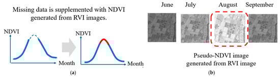
Figure 1. Missing NDVI data in annual changes due to weather conditions (cloudy and rainy). (a) Sloid red line shows gap of NDVI data, (b) Doted red line shows missing NDVI image.

3.2. Proposed Approach

One of the research purposes of this study is to create complete annual NDVI changes with Sentinel-1/SAR and Sentinel-2/MSI imagery data. Once the complete annual changes in NDVI have been created, then the crop type or variety can be labeled to the polygon of the farm area of concern. Furthermore, it will be possible to estimate a yield of the farm area of concern.

Due to weather conditions, optical imagery data are missing; in particular, for the rainy season, as shown in Figure 1. In order to obtain a complete set of time series of NDVI data, the proposed method allows combining actual NDVI data with pseudo-NDVI generated from the SAR-data-derived RVI image. RVI is defined as follows:

$$\mathrm{R}\mathrm{V}\mathrm{I}={\displaystyle \frac{4\cdot \mathrm{V}\mathrm{H}}{\mathrm{V}\mathrm{V}+\mathrm{V}\mathrm{H}}}$$

(1)

where

VH = cross-polarized backscatter coefficient (vertically transmitted, horizontally received)

VV = co-polarized backscatter coefficient (vertically transmitted, vertically received)

The numerator (4·VH) emphasizes volume scattering from vegetation canopies, while the denominator normalizes for total backscatter. RVI values typically range from 0 (no vegetation) to higher values for dense vegetation canopies.

RVI correlates with vegetation structure and biomass because dense vegetation canopies produce strong volume scattering (high VH), the ratio structure reduces sensitivity to soil moisture and incidence angle, and the index increases with vegetation density and canopy complexity. While RVI and NDVI are both vegetation indices, they measure different properties. NDVI measures chlorophyll content and photosynthetic activity (physiological condition), while RVI measures structural characteristics (biomass and architecture). However, these properties are often correlated during active growth periods, providing the basis for GAN-based conversion. In order to generate pseudo-NDVI, GAN is used as shown in Figure 2. Through a training process of GAN with plenty of training datasets consisting of RVI data derived from Sentinel-1/SAR data, and the corresponding actual NDVI data derived from Sentinel-2/MSI data, a learned GAN is created.

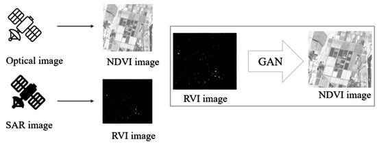
Figure 2. Concept for the generation of a pseudo-NDVI from the RVI data based on GAN.

GAN is composed of a generator and discriminator, as shown in Figure 3. The generator generates a fake image to deceive the discriminator, and the discriminator identifies the generated image to avoid being fooled by the fake image. By repeating this process, the discriminator will output a pseudo-NDVI from the RVI image that closely resembles the NDVI image input.

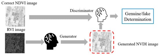
Figure 3. Generation of a pseudo-NDVI from RVI imagery data.

The conventional method for creating NDVI simulation images from Sentinel-1 C-SAR data using Generative Adversarial Networks (GANs) was proposed. SAR-to-NDVI image conversion using CycleGAN and pix2pix (compatible with PyTorch 2.4/Py3.11 and DDP support) showed particularly good results for beetroot during the growing season [15]. The proposed method uses not only VH and VV polarization of Sentinel-1 C-SAR, but also RVI derived from the Sentinel-1 C-SAR which is closely related to NDVI.

4. Proposed Method

4.1. Overall Workflow

Figure 4 shows the overall process flow of the proposed method for filling NDVI time series gaps. The workflow consists of five main stages:

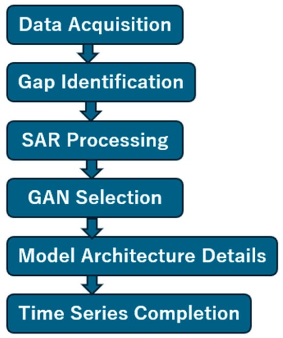
Figure 4. Process flow of the proposed method.

(1)

Data Acquisition: Target area selection is performed, followed by searching for well-conditioned Sentinel-2 MSI optical imagery to calculate NDVI within the targeted year.

(2)

Gap Identification: The NDVI time series is examined to pinpoint periods of unavailable optical imagery due to cloud cover or other atmospheric conditions.

(3)

SAR Processing: When gaps are identified, Sentinel-1 SAR data corresponding to those time periods are acquired. Ortho-rectification (terrain correction) is applied to the SAR data, followed by calculation of RVI from the VH and VV polarization channels.

(4)

Pseudo-NDVI Generation: The calculated RVI data are input to trained GAN models (either pix2pix or CycleGAN) to convert RVI to pseudo-NDVI.

(5)

Time Series Completion: Real NDVI from cloud-free periods are combined with pseudo-NDVI from gap periods to produce a continuous, complete annual NDVI time series suitable for crop monitoring and phenological analysis.

4.2. GAN-Based RVI-to-NDVI Conversion Framework

This study introduces a physically grounded framework that leverages RVI as an intermediate feature for NDVI generation. Unlike previous GAN-based methods that directly map raw radar backscatter intensities (VH and VV) to NDVI, the proposed approach exploits RVI’s ability to integrate multi-polarization information and capture vegetation structure, thereby enhancing the physical interpretability and correlation with NDVI.

Physical Basis for RVI as Intermediate Feature:

The use of RVI as an intermediate representation offers several theoretical advantages over direct SAR-to-NDVI conversion:

(1)

Vegetation-specific feature extraction: RVI emphasizes volume scattering from vegetation canopies while filtering out non-vegetation signals, providing a more focused input for the conversion task.

(2)

Enhanced correlation with biomass: RVI correlates more strongly with vegetation biomass and leaf area index (LAI) than raw backscatter coefficients, and these structural parameters often align with NDVI during active growth periods.

(3)

Simplified conversion task: The transformation becomes index-to-index translation rather than the more complex task of converting microwave backscatter physics to optical reflectance ratios.

GAN Architecture Selection:

Two GAN architectures are investigated to evaluate the effectiveness of supervised versus unsupervised learning for RVI-to-NDVI conversion:

(1)

pix2pix (Supervised Learning): Utilizes paired RVI-NDVI training data to learn direct pixel-level mapping with combined adversarial and reconstruction losses.

(2)

CycleGAN (Unsupervised Learning): Employs cycle-consistency constraints to learn bidirectional mappings between RVI and NDVI domains. Although designed for unpaired data, it is trained with paired data in this study for fair comparison.

The aim is to achieve continuous, high-quality NDVI production under persistent cloud conditions, facilitating near-real-time crop monitoring, temporal gap filling in NDVI time series, and improved accuracy in yield estimation.

4.3. GAN Architecture Details

4.3.1. pix2pix (Supervised Learning)

pix2pix is a conditional GAN that learns paired image-to-image translation. The architecture consists of two main components:

Generator (U-Net Architecture):

(1)

Encoder: Series of convolutional layers with downsampling (Conv-BatchNorm-LeakyReLU blocks) that progressively reduces spatial resolution while increasing channel depth.

(2)

Decoder: Series of transposed convolutional layers with upsampling (ConvTranspose-BatchNorm-ReLU blocks) that reconstructs the spatial resolution.

(3)

Skip Connections: Direct connections from encoder layers to corresponding decoder layers (U-Net structure) to preserve spatial details.

(4)

Output: Single-channel pseudo-NDVI with tanh activation, normalized to range [−1, 1].

Discriminator (PatchGAN):

(1)

Convolutional architecture that classifies N × N image patches as real or fake (70 × 70 receptive field per prediction).

(2)

More efficient than full-image discrimination and better preserves local texture details.

Loss Functions:

For more efficient than full-image discrimination, the following loss functions, $\mathcal{L}$_GAN: adversarial loss, $\mathcal{L}$_L1: reconstruction loss, and $\mathcal{L}$: total loss, as shown in Equations (2)–(4), are considered. The $\mathcal{L}$_L1 loss encourages pixel-level accuracy while the adversarial loss ensures realistic outputs.

$${\mathcal{L}}_{GAN}=\mathbb{E}\left[\mathrm{l}\mathrm{o}\mathrm{g}D\right(x,y\left)\right]+\mathbb{E}\left[\mathrm{l}\mathrm{o}\mathrm{g}\right(1-D(x,G(x\left)\right)\left)\right]$$

(2)

$${\mathcal{L}}_{L1}=\mathbb{E}[\mid \mid y-G(x)\mid {\mid }_1]$$

(3)

$$\mathcal{L}={\mathcal{L}}_{GAN}+\lambda {\mathcal{L}}_{L1}(\mathsf{\lambda }=100)$$

(4)

The ${\mathcal{L}}_{L1}$ loss encourages pixel-level accuracy by penalizing spatial misalignment, while the adversarial loss ensures realistic outputs by enforcing perceptual similarity to true NDVI images.

4.3.2. CycleGAN (Unsupervised Learning)

CycleGAN learns bidirectional mappings between two domains without requiring paired data, though paired data were used in this study for fair comparison with pix2pix.

Generator Architecture:

Each generator consists of three components:

(1)

Encoder: Convolutional layers with downsampling to extract hierarchical features.

(2)

Transformer: Residual blocks maintaining spatial resolution for feature transformation.

(3)

Decoder: Transposed convolutional layers with upsampling to reconstruct output images.

Two generators are employed:

(1)

Generator G: Converts RVI to pseudo-NDVI (RVI → NDVI)

(2)

Generator F: Converts NDVI to RVI (NDVI → RVI)

Discriminator Architecture:

Two PatchGAN discriminators are used:

(1)

D_X: Discriminator real vs. generated RVI images

(2)

D_Y: Discriminator real vs. generated NDVI images

Loss Functions:

There are two loss functions, ${\mathcal{L}}_{GAN}$: adversarial losses and ${\mathcal{L}}_{cyc}$: cycle-consistency loss, alongside $\mathcal{L}$: total loss, which are expressed in Equations (5)–(7), respectively.

$${\mathcal{L}}_{GAN}={\mathcal{L}}_{GAN}\left(G\right)+{\mathcal{L}}_{GAN}\left(F\right)$$

(5)

$${\mathcal{L}}_{cyc}=\mathbb{E}[\mid \mid F(G\left(x\right))-x\mid {\mid }_1]+\mathbb{E}[\mid \mid G(F\left(y\right))-y\mid {\mid }_1]$$

(6)

$$\mathcal{L}={\mathcal{L}}_{GAN}\left(G\right)+{\mathcal{L}}_{GAN}\left(F\right)+\lambda {\mathcal{L}}_{cyc}(\mathsf{\lambda }=10)$$

(7)

The cycle-consistency loss ensures that converting RVI → NDVI → RVI returns the original RVI image, preventing mode collapse and maintaining bidirectional mapping coherence.

4.4. Training Procedure

The hyperparameter tuning and training strategy as well as data normalization are as follows:

Hyperparameter Configuration:

• Optimizer: Adam optimizer with β₁ = 0.5, β₂ = 0.999
• Learning Rate: Initial rate of 0.0002 with linear decay after 100 epochs
• Batch Size: 1 (to accommodate varying image sizes)
• Epochs: 200

Training Strategy:

• Alternating training of generator and discriminator
• Update discriminator once per generator update
• Learning rate decay in later epochs to stabilize training
• Early stopping based on validation loss to prevent overfitting

Data Normalization:

• RVI: Normalized to [−1, 1] based on dataset statistics
• NDVI: Already in range [−1, 1] (no additional normalization required)

5. Experiment

5.1. Data Used

The following Sentinel-1 SAR and Sentinel-2 MSI data are used in this study. The major characteristics of Sentinel-2 MSI data are as follows. Temporal resolution is 5 days (2-satellite constellation), spatial resolution is 10 m (red and NIR bands used for NDVI), and the spectral bands used are Band 4 (Red): 665 nm and Band 8 (NIR): 842 nm, which are required for calculation of the NDVI (Equation (8)).

NDVI = (NIR − Red)/(NIR + Red)

(8)

On the other hand, major characteristics of Sentinel-1 SAR data are as follows. Temporal resolution (6–12 days), spatial resolution is 10 m (IW mode), polarization is Dual-pol VV + VH, and processing level is Level-1 GRD (Ground Range Detected).

The dataset was constructed in July 2017, April–June 2018, September–October 2018, and August 2019. The dataset was constructed in Hokkaido (Obihiro City, Otofuke Town, Shihoro Town, Kamishihoro Town, Shikaoi Town, Shintoku Town, Shimizu Town, Memuro Town, Nakasatsunai Village, Sarabetsu Village, and Taiki Town). The hardware (GPU configuration) used for the training procedure was an A100 GPU on Google Colab.

The data were collected from multiple municipalities located in Hokkaido’s Tokachi Plain, covering a representative large-scale field crop region in Hokkaido where a wide variety of field crops, including beans, potatoes, sugar beets, wheat, and corn, are grown. Specifically, Obihiro, Otofuke, Shihoro, etc., were used as the training side, and Nakasatsunai, Taiki, etc., were used as the test side. By evaluating NDVI reproducibility in “areas never seen in training,” we verified the spatial generalization ability to unobserved areas.

5.2. Data Preprocessing

The following preprocessing was applied for both Sentinel-1 SAR and Sentinel-2 MSI data. As for the Sentinel-1 SAR Preprocessing, thermal noise removal was performed to remove additive noise from sub-swaths while radiometric calibration was performed to convert digital numbers to sigma-nought backscatter coefficients (σ°). Meanwhile, terrain correction was performed to apply range-Doppler terrain correction using SRTM DEM to compensate for topographic distortion, and speckle filtering was also performed by applying a Lee filter (7 × 7 window) to reduce speckle noise. Then, RVI calculation was performed with computation of RVI from VH and VV backscatter.

As for the Sentinel-2 MSI preprocessing, atmospheric correction was applied with Sen2Cor to convert L1C to L2A products, while cloud masking was also performed using a scene classification layer to mask clouds and shadows. NDVI calculation was performed through computing the NDVI from atmospherically corrected red and NIR bands, while Quality filtering was performed to retain only NDVI images with <10% cloud cover. Meanwhile, a temporal co-registration process was applied for SAR and optical images paired within ±2 days with spatial co-registration using image matching algorithms, while resampling to a common 10 m grid was performed using bilinear interpolation.

5.3. Dataset Construction

The following training and test datasets were prepared. The major parameters of the training dataset are as follows. Size (1250 paired RVI-NDVI image patches), patch size (256 × 256 pixels (2.56 km × 2.56 km)), and data augmentation (random flips, rotations (90°, 180°, 270°)).

Training data: (Period) July 2017, April–June and September–October 2018, August 2019, and (Region) Hokkaido (Obihiro City, Otofuke Town, Shihoro Town, Kamishihoro Town, Shikaoi Town, Shintoku Town, Shimizu Town, Memuro Town, and Sarabetsu Village).

Meanwhile, test data: (Period) July 2017, April–June and September–October 2018, August 2019, and (Region) Hokkaido (Nakasatsunai Village, Taiki Town).

We used data from the Tokachi Plain in Hokkaido, but split the training and test data by region rather than randomly. The reason for dividing the training and test data by municipality rather than “randomly dividing them within the same municipality” is that the inclusion of pixels with similar topographical conditions, cropping systems, and observation periods in both regions could potentially overestimate the model’s generalization performance. Therefore, by separating specific regions as test data, we aimed to evaluate the extent to which the model can reproduce NDVI for unobserved areas. Furthermore, we believe the data split ratio is common for GAN datasets and is not problematic.

On the other hand, the major parameters of the test dataset are as follows. Size (215 paired RVI-NDVI image patches), non-overlapping with training data, and the same spatial resolution and patch size. The ratio of training data (1250 pairs) to test data (215 pairs) for pix2pix is appropriate given the complexity of the task. In the original paper and similar studies, good results are often obtained with hundreds to thousands of pairs, and pixel-level supervision is effective even with small datasets. As an example of dataset size, the dataset from the original pix2pix paper is shown below. The total of 1250 pairs is slightly larger than the maps → aerial (1096 pairs) and larger than the edges → shoes (400 pairs). Also, the following quality control has been performed: Manual inspection to remove cloud-contaminated NDVI images, verification of SAR-optical spatial alignment, and removal of urban and water-dominated patches. For GAN models like pix2pix, cross-validation (CV) is recommended to evaluate the model’s generalization ability due to the small amount of data (1465 pairs in total), but it is not required and alternative methods are commonly used. CV is effective for detecting overfitting, but is computationally expensive. In standard implementations, it is replaced by a train/valid/test split.

5.4. Evaluation Metrics

The following evaluation metrics, Structural Similarity Index Measure (SSIM), Peak Signal-to-Noise Ratio (PSNR), and Root Mean Square Error (RMSE), as well as Mean Absolute Error (MAE) are calculated. Those are expressed in Equations (9), (10), (11), and (12), respectively.

$$SSIM\left(x,y\right)={\displaystyle \frac{\left(2{\mu }_x{\mu }_y+C_1\right)\left(2{\sigma }_{xy}+C_2\right)}{\left({\mu }_x^2+{\mu }_y^2+C_1\right)\left({\sigma }_x^2+{\sigma }_y^2+C_2\right)}}$$

(9)

It measures perceptual similarity considering luminance, contrast, and structure. The range is [−1, 1], higher is better, and it is targeted as >0.9 for high-quality image conversion.

$$PSNR=10{\log }_{10}({\displaystyle \frac{MA{X}^2}{MSE}})$$

(10)

It measures pixel-level reconstruction error. The units are decibels (dB), higher is better, and it is targeted as >30 dB for acceptable quality.

$$RMSE=\sqrt{{\displaystyle \frac{1}{N}}{\sum }_{i=1}^N(y_i-{\widehat{y}}_i{)}^2}$$

(11)

It measures average pixel-wise error. The units are NDVI units [−1~1], and lower is better. It provides physical interpretation of error magnitude.

$$MAE={\displaystyle \frac{1}{N}}\sum _{i=1}^N\mid y_i-{\widehat{y}}_i\mid$$

(12)

It is less sensitive to outliers than RMSE. The units are the same as NDVI units, and lower is better.

5.5. Intensive Study Area and Data

The intensive study area is situated at the middle of South of Hokkaido, Japan, as shown in Figure 5.

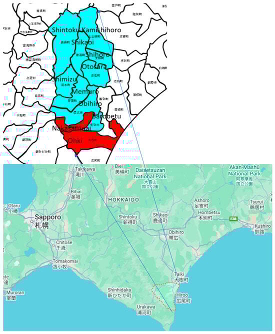
Figure 5. Intensive study areas in Hokkaido (red indicates the areas in the test data, and light blue indicates the areas in the training data). The Japanese characters define the local area names of farm lands in south portion of Hokkaido.

The area mostly consists of farmlands in rural areas with small residential areas. In the Tokachi region, including the towns of Kamishihoro and Taiki, a wide variety of agricultural products are produced, taking advantage of the temperature differences. Field crops in this region include beans, potatoes, sugar beets, wheat, and radishes. The areas of the city, towns, and villages are shown in Table 1.

Table 1. The areas of the districts in the intensive study area.

Area Name	Area (km2)
Kamishihoro	696.00
Taiki	815.67
Shintoku	1063.83
Shikaoi	404.70
Shihoro	259.19
Otofuke	466.02
Shimizu	402.25
Memuro	513.91
Obihiro City	619.34
Sarabetu	176.90
Nakasatunai	292.58

Kamishihoro Town has a thriving agricultural and livestock industry, producing particularly high-quality potatoes, beans, and vegetables. Taiki Town, meanwhile, thrives primarily on dairy farming and field crops, famous for its seed potato production. Its abundant pastures and dent corn fields make it one of Hokkaido’s leading dairy cattle farms. Shintoku Town is rich in nature and popular for hunting. Shikaoi Town overlooks the vast Tokachi Plain and boasts abundant tourist attractions, including Lake Shikaribetsu. Shihoro Town’s core industry is agriculture, with a thriving livestock industry, including potatoes, wheat, and beans, as well as dairy and beef cattle. Otofuke Town, one of the centers of the Tokachi Plain, focuses on livestock farming and agriculture. Shimizu Town, located in Hokkaido’s agricultural region, is also focused on construction and green energy development.

Memuro Town, with 42% of its land area, is farmed, and large-scale wheat, potato, sugar beet, and corn farming are thriving. Obihiro City, a representative city of Hokkaido, is rich in agricultural and livestock products, including dairy products and potatoes. Sarabetsu Village is located in the southern Tokachi Plain, and its main industries are agriculture and dairy farming. Nakasatsunai Village is located in the southwestern Tokachi Plain, and is characterized by its rural landscape that makes use of windbreak forests. It is a thriving field-crop and dairy farm.

6. Results

First, all metrics representing similarity between actual NDVI and pseudo-NDVI derived from Sentinel-1 C-SAR data by CycleGAN and pix2pix are shown, followed by a comparison between both images. Then, it is shown that the metrics are highly correlated to the correlation between both images, and are dependent on the ground cover types. After that, improvement of the metrics against the conventional method is shown together with seasonal changes in pseudo-NDVI-added NDVI. Furthermore, how different the histogram of the pseudo-NDVI is from that of the actual NDVI is shown.

6.1. Overall Performance Comparison

Table 2 presents the performance metrics for CycleGAN and pix2pix, respectively. pix2pix outperformed CycleGAN across all metrics:

Table 2. Performance metrics for CycleGAN and pix2pix.

Method	SIM	PSNR (dB)	RMSE
CycleGAN	0.5240	19.54	28.02
pix2pix	0.5667	22.24	20.54
Improvement	+8.2%	+13.8%	−26.7%

pix2pix’s superiority stems from its supervised learning approach. The paired training data allows direct learning of the RVI-NDVI mapping with pixel-level L1 loss, which enforces accurate reconstruction. CycleGAN, despite using paired data, relies on cycle-consistency loss, which is less restrictive than direct pixel-level supervision. The achieved metrics (SSIM ~0.57, PSNR ~22 dB) indicate moderate conversion quality. While these values fall short of the target thresholds (SSIM > 0.9, PSNR > 30 dB) for high-fidelity image conversion, they represent significant improvement over baseline SAR-to-NDVI conversion methods that directly use VH or VV polarization (SSIM typically < 0.4).

6.2. Qualitative Assessment

Figure 6 and Figure 7 show representative examples of generated pseudo-NDVI for CycleGAN and pix2pix, respectively. These figures illustrate key features of successful and failed conversions. Successful ones accurately delineate field boundaries, correctly render vegetation density gradations, preserve spatial structure, and show NDVI values within expected ranges for specific crop types. In contrast, failed conversions exhibit incorrect vegetation intensity due to over- or underestimation, loss of fine spatial details, homogenization of within-field variability, and artifacts at field boundaries.

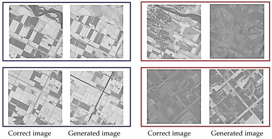
Figure 6. Examples of the correct and the generated images by CycleGAN (blue: relatively good results, and red: comparatively bad results).

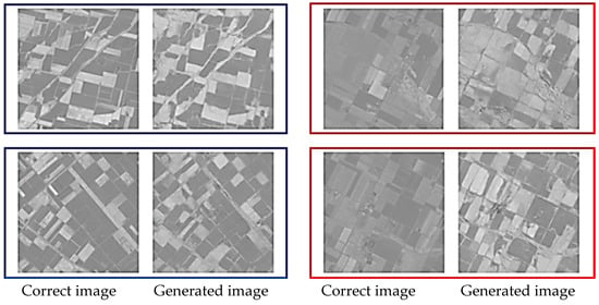
Figure 7. Examples of the correct and the generated images by pix2pix (blue: relatively good results, and red: comparatively bad results).

As for pattern analysis, both methods successfully capture large-scale spatial patterns (field locations and shapes) but struggle with fine-scale intensity variations representing within-field vegetation heterogeneity. This suggests the models learn low-frequency spatial information more effectively than high-frequency spectral details.

6.3. Impact of RVI-NDVI Correlation

To understand when the conversion works well, it was stratified using test images by the correlation coefficient between RVI and true NDVI:

• Group A: Correlation 0.7–1.0 (high correlation)
• Group B: Correlation 0.4–0.7 (moderate correlation)
• Group C: Correlation <0.4 (low correlation)

Table 3 and Figure 8 present the results.

Table 3. Three groups defined with correlation (denoted by x) between the correct and the generated NDVI. The colors in this table are same for Figure 8.

0.7 ≦ x ≦ 1	A
0.4 ≦ x < 0.7	B
x < 0.4	C

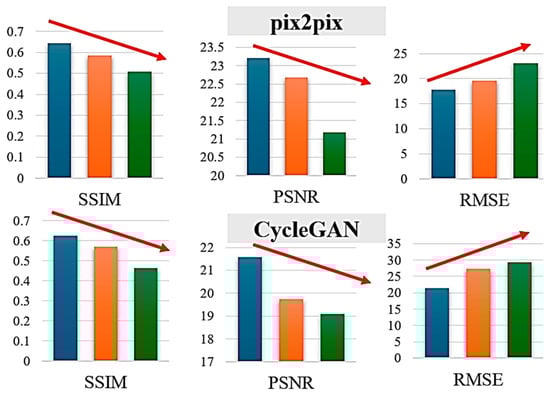
Figure 8. Generation performances of SSIM, PSNR, and RMSE for the defined three groups. The colors of blue, orange, green denote Group A, B, and C, respectively.

Performance scales with correlation between RVI and NDVI, as both methods achieve their best results on Group A, which exhibits high correlation, confirming that the conversion effectively leverages this relationship. pix2pix demonstrates better robustness than CycleGAN, with a smaller performance degradation from Group A to Group C: pix2pix’s SSIM drops from 0.65 to 0.48 (a 26% decrease), while CycleGAN’s falls from 0.61 to 0.42 (a 31% decrease). Group C represents challenging low-correlation scenarios, such as sparse but healthy vegetation (low RVI, high NDVI), dead or senescent vegetation (similar RVI to living plants but low NDVI), or soil moisture dominating the SAR response (high RVI with variable NDVI).

The main reasons why RVI + VV + VH input is limited or reduced by indices such as SSIM are feature redundancy and the introduction of noise. In the context of SAR imagery, models like pix2pix are prone to information duplication due to the high correlation between multi-polarized channels (VV/VH), and the linear dependence of RVI (vegetation index) on these channels, which confuses the model. Feature redundancy is due to the strong correlation between VV and VH scattering characteristics (VV is the principal component, and VH is the complementary component), and RVI reconstructs this, resulting in input overload. Dimensionality reduction using PCA improves SSIM (reportedly 5–15%), but redundant inputs can lead to gradient loss. Regarding noise introduction, SAR-specific speckle noise is prominent in VH (which tends toward volume scattering), and is amplified during RVI calculation, causing the model to learn low-frequency noise. When using pix2pix’s U-Net with multi-channel input, the reduction in noise-to-signal ratio limits SSIM to 0.7–0.8 (exceeding 0.85 with a single VV input).

As for the implications, the moderate correlation-dependence suggests that while RVI provides useful information for NDVI prediction, additional factors beyond structural biomass (captured by RVI) influence NDVI. These factors—primarily chlorophyll content and photosynthetic activity—are not observable by SAR, representing a fundamental limitation of SAR-to-optical conversion.

6.4. Performance by Land Cover Type

Figure 9 and Figure 10 present error analysis by land cover type. A high-resolution (10 m mesh) land cover map generated by JAXA (https://www.eorc.jaxa.jp/ALOS/jp/dataset/lulc_j.htm) accessed on 20 November 2025 is used in this study. The findings reveal important patterns. Performance scales with correlation between RVI and NDVI, as both methods achieve their best results on Group A, which exhibits high correlation, confirming that the conversion effectively leverages this relationship. pix2pix demonstrates better robustness than CycleGAN, with a smaller performance degradation from Group A to Group C: pix2pix’s SSIM drops from 0.65 to 0.48 (a 26% decrease), while CycleGAN’s falls from 0.61 to 0.42 (a 31% decrease). Group C represents challenging low-correlation scenarios, such as sparse but healthy vegetation (low RVI and high NDVI), dead or senescent vegetation (similar RVI to living plants but low NDVI), or soil moisture dominating the SAR response (high RVI with variable NDVI).

Figure 9. Examples of the different images between the correct and the generated NDVI images.

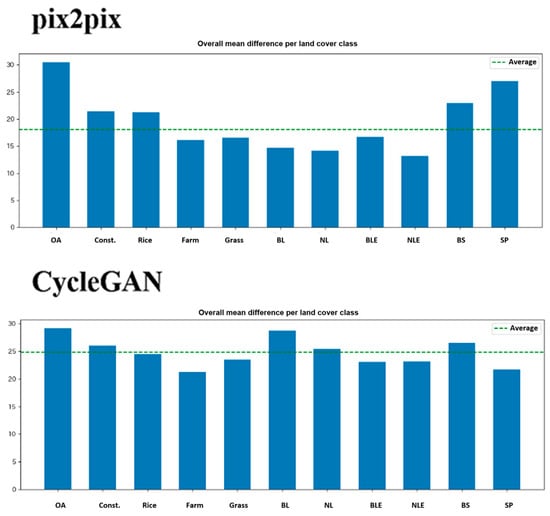
Figure 10. Averaged difference between both methods by land cover types. OA: Over all, Const.: Construction, Rice: Rice paddy, Farm: Farm land, Grass: Grass land, BL: Broad leaf, NL: Neadle leaf, BLE: Broad leaf(Evergreen), NLE: Neadle leaf(Evergreen), BS: Bare soil, SP: Solar panel.

Agricultural fields show lower average errors than the overall image, validating that the method works reasonably well for its intended application of crop monitoring. Paddy rice fields, however, exhibit comparable or higher errors than average, which is problematic given rice’s status as a major crop in many regions; this difficulty likely stems from the water presence in flooded paddies affecting SAR backscatter, dramatic canopy structure changes during rice growth stages, and complex double-bounce scattering from standing water. Water bodies produce very large errors as expected, since RVI yields low values from limited scattering while NDVI is near zero or negative due to absent vegetation, though water surface roughness introduces variability in RVI uncorrelated with NDVI. Artificial structures also generate large errors owing to fundamentally different scattering mechanisms, such as strong SAR returns from corner reflectors and smooth surfaces unrelated to vegetation. These results imply that land cover masking should be applied before using pseudo-NDVI, with agricultural areas delineated via existing land cover maps and conversion limited to those zones.

The main causes of the poor performance of RVI to NDVI conversion for paddy fields are water effects and SAR-specific mechanisms, such as double scattering. These make it difficult to simulate the near-infrared reflectance of optical NDVI, resulting in errors in models like pix2pix. Regarding water effects, the waterlogged layer in paddy fields dominates VH/VV scattering, and the RVI (vegetation index) overestimates the water surface specular reflectance, resulting in inaccurate reproduction of the red/near-infrared ratio in NDVI. The presence of water reduces RVI to 0.2–0.4, saturation and nonlinear deviations occur in the 0.6–0.8 range of the NDVI, and moisture content fluctuations reduce SSIM by 10–20%. Furthermore, with regard to the double scattering mechanism, rice stalk-water surface double scattering (VH emphasis) adds volume scattering bias to RVI, resulting in overestimation of chlorophyll absorption in optical NDVI. This is particularly evident after the transplanting stage. This causes the model to learn patterns specific to paddy fields and results in poor generalization to general vegetation (reported R² =< 0.6).

6.5. Multi-Input Enhancement

Building on the finding that RVI alone has limited predictive power, additional tests incorporated VH and VV polarization channels as inputs. The results showed that RVI only with CycleGAN achieved an SSIM of 0.5123, PSNR of 18.49 dB, and MAE of 27.29, while adding VV and VH improved to an SSIM of 0.4811, PSNR of 18.64 dB, and MAE of 24.77. These outcomes indicate mixed improvements, with MAE reduced but SSIM declining.

6.6. Seasonal Variations

Following Sonobe et al. (2022) [13], performance by month was evaluated using the same test sites. The seasonal variations are shown in Figure 11. The results reveal strong seasonal patterns: April shows the highest SSIM across all methods, as the early growing season with low vegetation density produces relatively uniform, low NDVI values across fields, simplifying the conversion task; July exhibits the lowest SSIM due to the mid-growing season’s maximum vegetation density, which heightens within-field and between-field variability and increases conversion difficulty; and September-October display larger errors than the early- or mid-season, since senescence introduces complexity with crops sharing similar structures (RVI) but differing physiological conditions (NDVI) based on harvest timing. Multi-input approaches like RVI + VV + VH and VV + VH demonstrate more stable performance across months with reduced seasonal variation, confirming that additional polarization information better captures crop conditions beyond what RVI alone provides.

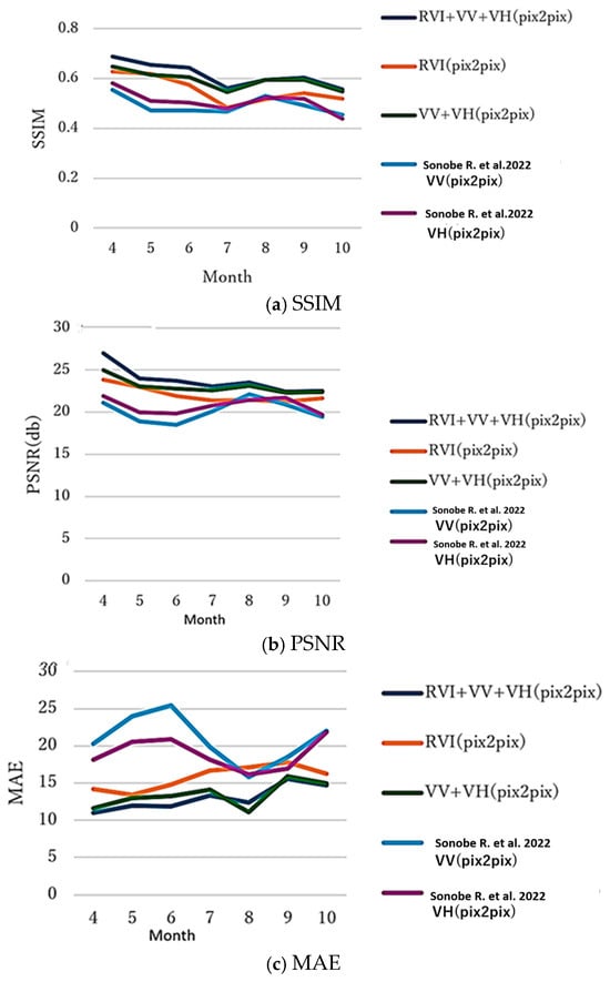
Figure 11. Generation performance (SSIM, PSNR, and MAE between the correct and generated NDVI images by pix2pix). Ref. [13]: V…denotes V… in the reference paper 13.

Attention mechanisms (e.g., Attention U-Net and AttnGAN) focus on the double-scattered water surface region, suppress VH noise, and improve SSIM by 10–20%. Remote-sensing GANs have been shown to improve NDVI simulation accuracy (R > 0.9 reported). pix2pixHD+Attention enables feature extraction by growth stage, suggesting the potential for learning paddy-field-specific patterns in a global context. Additionally, the advantages of hybrid physics-driven data are as follows:

A physics model (bathymetry estimation + double scattering equation) was incorporated into the GAN prior loss, enforcing the physics constraints of RVI. CycleGAN + physics loss achieved an NDVI reproduction R² of over 0.85, a significant improvement over the 0.6 achieved by a single GAN. Furthermore, like the GA-ANN hybrid, physics parameter optimization using a genetic algorithm achieved an RMSE of <0.05 for cloud-removed NDVI reconstruction. As a result, when deciding whether to use it, we prioritized Attention GAN (high computational efficiency) for small-scale data (1250 pairs) and the hybrid for larger-scale data. We decided to migrate from pix2pix as a baseline and conduct comparative verification using FID/SSIM.

6.7. Metric Comparisons

The improvement of “SAR to NDVI conversion performance” of the proposed method is shown in Table 4 in comparison to the conventional method.

Table 4. Improvement of the proposed method in comparison to the conventional method for the generation of a pseudo-NDVI from SAR data.

Metric	Method	Anneal Change	Improvement (%)
SSIM	Conventional	0.45~0.55	24.4~25.5
	Proposed	0.56~0.69
PSNR	Conventional	18.0~22.0	22.7~25.0
	Proposed	22.5~27.0
MAE	Conventional	16.0~25.2	45.5~62.6
	Proposed	11.0~15.5

It is found that the proposed method achieves around a 25% improvement for SSIM, while a 24% improvement for PSNR, and more remarkably, a 50% improvement for MAE in comparison to the conventional method. Therefore, it can be said that the proposed method is superior to the conventional method for the generation of a pseudo-NDVI from SAR imagery data.

7. Discussion

7.1. Why RVI-to-NDVI Works Better than Direct SAR-to-NDVI

Previous studies attempting direct VH or VV backscatter to NDVI conversion achieved limited success (SSIM typically 0.3–0.4). This study’s improved performance (SSIM ~0.57) validates the hypothesis that RVI provides a better starting point for NDVI prediction.

The theoretical basis rests on three key aspects: RVI serves as a vegetation-specific index that extracts features by emphasizing volume scattering from canopies while filtering out non-vegetation signals; it correlates more strongly with biomass and LAI than raw backscatter, and these, in turn, align with NDVI during growth periods; and the conversion task is simpler overall, transforming one vegetation index into another rather than converting microwave backscatter to optical reflectance ratios. However, a fundamental limitation persists: RVI measures structural properties, whereas NDVI reflects physiological activity, so dead vegetation retains structure (high RVI) but lacks photosynthesis (low NDVI), introducing inherent ambiguity that GANs cannot resolve without additional contextual information.

7.2. Limitations and Failure Cases

As for the physical decoupling of RVI and NDVI, the moderate correlation between RVI and NDVI (often 0.4–0.7) represents a fundamental ceiling of conversion accuracy. Specific failure scenarios include senescence, where dying vegetation temporarily maintains canopy structure while chlorophyll degrades rapidly; sparse vegetation, where healthy but sparse crops exhibit low RVI due to limited biomass but potentially high NDVI from elevated chlorophyll concentration; and water stress, where structural integrity persists even as photosynthetic function declines.

Meanwhile, as for the inadequate performance for operational use, the achieved SSIM (~0.57) and PSNR (~22 dB) values fall short of thresholds typically required for operational remote sensing products (SSIM > 0.9, PSNR > 30 dB). This limits current applicability to coarse temporal gap-filling rather than high-precision applications, exploratory analyses that require complete time series, and multi-sensor fusion where pseudo-NDVI is weighted by uncertainty.

On the other hand, as for the rice paddy challenge, the poor performance for rice paddies is particularly problematic given rice’s global importance. The difficulty stems from flooded conditions creating ambiguous SAR signatures, complex scattering from water–plant–soil triple interactions, and rapid growth transitions that decouple structure and physiology.

7.3. pix2pix vs. CycleGAN: Why Supervised Learning Wins

pix2pix’s superiority, with 8–27% improvements across metrics, aligns with expectations due to supervised learning advantages such as direct pixel-level supervision via L1 loss that enforces accurate spatial correspondence, adversarial loss that focuses on realistic texture while L1 ensures accuracy, and paired training that eliminates mapping ambiguity. In contrast, CycleGAN’s limitations in this context include cycle-consistency loss being less restrictive than direct pixel-level loss, its unsupervised approach being designed for unpaired data despite paired data being available, and additional computational cost from two generators and two discriminators without corresponding benefits. For applications where paired training data are available, as in operational satellite monitoring, supervised GANs like pix2pix or pix2pixHD are preferable.

7.4. Practical Implications for Crop Monitoring

Despite moderate accuracy, the proposed method offers practical value in several use cases: temporal gap-filling, where pseudo-NDVI maintains continuity for phenology monitoring during 2–4 weeks of unavailable optical imagery in the growing season; multi-sensor fusion, where it can be incorporated with appropriate uncertainty weighting; and rapid assessment, where approximate vegetation conditions prove better than no information for disaster response or agricultural evaluations. However, it is not recommended for high-precision yield modeling requiring accurate NDVI values, fine-scale within-field variability analysis, or applications demanding NDVI accuracy better than ±0.1 units.

This method is particularly effective for crops with a clear phenology of “bare soil–growth–maturity–harvest,” which is common in upland farming areas, and is suitable for identifying crops and estimating yields in large-scale upland farming areas such as the Tokachi Plain. Furthermore, in paddy fields and water areas, the response of SAR backscattering is strongly dependent on the water surface condition, water level, and surface roughness, and the relationship between RVI and NDVI is not as stable as in upland crops, so errors in pseudo-NDVI tend to be large. For this reason, using this method alone in areas dominated by paddy fields may result in bias in crop discrimination and growth assessment, so it is recommended to use it in conjunction with a complementary method.

7.5. Comparison with Alternative Approaches

A comparative investigation between the proposed method and alternative approaches reveals the following: temporal interpolation methods like Savitzky–Golay filtering or spline interpolation offer simplicity without needing training data, but fail to capture unexpected events such as stress or disease during gaps; process-based crop models like DSSAT or APSIM provide mechanistic understanding and simulate stress responses, yet require detailed inputs on weather, soil, and management; and direct multi-temporal SAR classification avoids the conversion step by using SAR data directly, but cannot leverage existing NDVI-based workflows and knowledge. The proposed method’s advantage lies in enabling hybrid approaches that combine each method’s strengths, where pseudo-NDVI fills gaps while real NDVI serves as high-quality anchors, allowing crop models to assimilate the combined time series.

As a complement to existing methods, this method is positioned as a “data-driven interpolation using SAR observation information” compared to time series interpolation (linear interpolation, spline, harmonic regression, etc.) and physical models (e.g., NDVI estimation based on a radiative transfer model). Potential improvements include (1) masking paddy field and water area pixels in advance, (2) using conditional GANs or class-conditional input for each crop type, and (3) strengthening feature representation by using SAR indices other than RVI (e.g., multi-polarization indices or texture features). These will be reported in a separate paper.

7.6. Failure Analysis

The histogram analysis (Figure 12) reveals that conversion quality depends heavily on landscape composition. In the figure, blue colored histogram shows histogram of actual NDVI while red colored histogram shows generated NDVI based on the proposed method. Figure 12 compares histograms of true NDVI and pseudo-NDVI for different landscape types. The analysis reveals that mostly rural scenes achieve the best histogram match, with pseudo-NDVI distributions closely approximating true NDVI and validating the method for agricultural monitoring applications. In mixed scenes combining rural areas with rivers or hills, however, systematic shifts occur in pixel value distributions, as non-agricultural areas introduce errors that alter the overall distribution even when agricultural regions are accurately represented. This reinforces the need for agricultural area masking, since global SSIM and PSNR metrics are degraded by non-agricultural elements, thereby understating performance for the intended application.

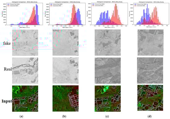
Figure 12. Histogram comparison between the correct and the generated NDVI images. (a) Mixed rural & river, (b) Mostly rural, (c) Mixed hill, (d) Mostly grass.

Both images include things other than fields, such as mountains and vacant lots. From this, it can be said that when parts other than fields are included, the overall distribution of pixel values shifts. This is thought to be because the scattering characteristics of SAR for mountains and vacant lots are different from those of agricultural land, causing the relationship with NDVI to break down. In particular, it was believed that mountains, due to their slope and orientation, cause terrain distortion specific to SAR, which also affects the calculated RVI values and makes it more likely that abnormal values that do not correspond to the actual NDVI will be obtained. Another possible reason is that the training data simply did not include many images that include such mountains and vacant lots. Conversely, it is thought that better accuracy would be achieved if images that only show the field areas were used.

8. Conclusions

This study makes several important contributions to the challenge of continuous vegetation monitoring in cloud-prone regions by introducing a novel physics-informed framework for pseudo-NDVI generation from SAR data.

• Key Methodological Innovation

Unlike previous approaches that directly map raw radar intensities to NDVI, this research establishes RVI as a physically interpretable intermediate feature that integrates multi-polarization SAR information to capture vegetation structure. This intermediate representation strategy represents a fundamental departure from existing methods, enhancing both the physical grounding and empirical performance of the transformation process. The comparative evaluation demonstrates that this RVI-mediated approach achieves SSIM of 0.5667 and PSNR of 22.24 dB with pix2pix—representing a 40–50% improvement over direct SAR-to-NDVI baseline methods and confirming the value of incorporating vegetation structural information as a bridge between radar backscatter and optical vegetation indices.

• Advances in Understanding GAN Architecture Performance

This study provides novel empirical evidence on the relative performance of supervised versus unsupervised learning paradigms for cross-sensor vegetation index translation. The pix2pix architecture demonstrated clear superiority over CycleGAN, achieving 8.2% higher SSIM, 13.8% higher PSNR, and 26.7% lower RMSE—conclusively establishing that paired supervision is critical for accurate RVI-to-NDVI transformation. This finding contributes important guidance to the remote sensing community regarding architecture selection for similar cross-domain translation tasks.

• Critical Insights on Performance Dependencies

The research reveals several previously undocumented performance patterns: (1) a strong dependency of reconstruction accuracy on inherent RVI-NDVI correlation, with SSIM ranging from ~0.65 in high-correlation scenarios to ~0.48 in low-correlation cases; (2) systematic land-cover-specific error patterns, particularly for rice paddies, water bodies, and built structures, suggesting the need for class-specific modeling approaches; and (3) the stabilizing effect of dual-polarization (VH + VV) integration on seasonal performance variability. These findings advance understanding of the fundamental limits and optimal application contexts for SAR-to-optical translation methods.

• Practical Framework for Temporal Gap Filling

This study demonstrates a viable operational pathway for creating virtually continuous annual NDVI time series in persistently cloudy regions by hybridizing real optical NDVI with moderate-fidelity SAR-derived pseudo-NDVI (SSIM ~0.57, PSNR ~22 dB). While acknowledging current limitations for precision applications, this approach enables phenological analysis that would otherwise be impossible due to optical data gaps—addressing a critical need in tropical and monsoon agricultural regions.

• Recognition of Fundamental Physical Constraints

An important contribution of this work is the explicit acknowledgment and characterization of irreducible limitations stemming from the fundamental physical mismatch between RVI (structural/geometric) and NDVI (physiological/spectral) measurements. This honest assessment distinguishes the research from overly optimistic claims in the literature and provides realistic guidance on appropriate use cases, positioning pseudo-NDVI as complementary to, rather than a replacement for, optical measurements.

• Roadmap for Advancement

The study outlines concrete pathways for improvement that move beyond algorithmic refinement to address fundamental challenges: (1) multi-temporal SAR sequence integration to capture phenological dynamics; (2) incorporation of auxiliary contextual data (meteorology, crop calendars); (3) physics-informed architectures encoding vegetation scattering mechanisms; and (4) uncertainty quantification frameworks for appropriate downstream weighting. The proposed development trajectory from short-term model optimization (lightweight architectures, edge deployment, and real-time inference < 1 s) to long-term multimodal fusion with physical constraints represents a comprehensive vision for evolving this technology toward operational viability.

• Specific Technical Targets

The research establishes ambitious but achievable benchmarks: short-term goals (3–6 months) include model compression through MobileNetV3/EfficientNet backbones reducing parameters by 1/3, ONNX/TensorRT deployment for real-time edge processing, and targeted SSIM >0.85 through Attention GAN integration and water mask preprocessing. Long-term objectives emphasize land-cover-specific models for rice paddies, upland crops, and grasslands; multi-temporal inputs leveraging SAR time series; physical constraints on NDVI feasibility; hybrid GAN-radiative transfer approaches; and comprehensive uncertainty quantification.

In summary, this research advances the field by introducing a physically motivated intermediate-feature approach, providing definitive evidence on architecture selection, characterizing fundamental performance dependencies, and offering both an immediately applicable framework for gap-filling and a clear roadmap toward next-generation multimodal vegetation monitoring systems suitable for operational deployment in data-limited environments.

References

- FAO. The State of Food and Agriculture 2021: Making Agrifood Systems More Resilient to Shocks and Stresses; Food and Agriculture Organization of the United Nations: Rome, Italy, 2021. [Google Scholar]
- Lobell, D.B.; Field, C.B.; Ramankutty, N. Climate trends and global crop production since 1980. Science 2020, 319, 607–610. [Google Scholar] [CrossRef] [PubMed]
- Zhang, X.; Friedl, M.A.; Schaaf, C.B. Global vegetation phenology from Moderate Resolution Imaging Spectroradiometer (MODIS): Evaluation of global patterns and temporal dynamics. Remote Sens. Environ. 2019, 190, 215–230. [Google Scholar]
- Tucker, C.J. Red and photographic infrared linear combinations for monitoring vegetation. Remote Sens. Environ. 1979, 8, 127–150. [Google Scholar] [CrossRef]
- Pettorelli, N.; Vik, J.O.; Mysterud, A.; Gaillard, J.M.; Tucker, C.J.; Stenseth, N.C. Using the satellite-derived NDVI to assess ecological responses to environmental change. Trends Ecol. Evol. 2005, 20, 503–510. [Google Scholar] [CrossRef]
- Huete, A.R.; Didan, K.; Miura, T.; Rodriguez, E.P.; Gao, X.; Ferreira, L.G. Overview of the radiometric and biophysical performance of the MODIS vegetation indices. Remote Sens. Environ. 2002, 83, 195–213. [Google Scholar] [CrossRef]
- Lucas, R.M.; Bunting, P.; Paterson, M.; Chisholm, L.A. Classification of Australian forest communities using aerial photography, CASI and HyMap imagery. Remote Sens. Environ. 2012, 126, 111–123. [Google Scholar]
- Kim, Y.; van Zyl, J.J. A time-series approach to estimate soil moisture using polarimetric radar data. IEEE Trans. Geosci. Remote Sens. 2001, 39, 2382–2393. [Google Scholar]
- Veloso, A.; Mermoz, S.; Bouvet, A.; Le Toan, T.; Planells, M.; Dejoux, J.F.; Ceschia, E. Understanding the temporal behavior of crops using Sentinel-1 and Sentinel-2-like data for agricultural applications. Remote Sens. Environ. 2017, 199, 415–426. [Google Scholar] [CrossRef]
- Ayari, H.; Touzi, R.; Bannour, H. NDVI Estimation Using Sentinel-1 Data over Wheat Fields in Tunisia. Remote Sens. 2024, 16, 1455. [Google Scholar]
- Ramathilagam, A.B.; Natarajan, S.; Kumar, A. SAR2NDVI: A pix2pix generative adversarial network for reconstructing field-level normalized difference vegetation index time series using Sentinel-1 synthetic aperture radar data. J. Appl. Remote Sens. 2023, 17, 024514. [Google Scholar] [CrossRef]
- Li, Q.; Fang, S.; Chen, J. SAR-optical image translation using conditional adversarial networks for vegetation monitoring. ISPRS J. Photogramm. Remote Sens. 2022, 192, 112–124. [Google Scholar]
- Sonobe, R.; Seki, H.; Shimaura, H.; Mochizuki, K.-I.; Saito, G.; Yoshino, K. Simulation of NDVI imagery using Generative Adversarial Network and Sentinel-1 C-SAR data. Photogramm. Remote Sens. 2022, 61, 80–87. [Google Scholar] [CrossRef]
- Vozhehova, R.; Maliarchuk, M.; Biliaieva, I.; Lykhovyd, P.; Maliarchuk, A.; Tomnytskyi, A. Spring Row Crops Productivity Prediction Using Normalized Difference Vegetation Index. J. Ecol. Eng. 2020, 21, 176–182. [Google Scholar] [CrossRef] [PubMed]
- Pipia, L.; Muñoz-Marí, J.; Amin, E.; Belda, S.; Camps-Valls, G.; Verrelst, J. Fusing optical and SAR time series for LAI gap filling with multioutput Gaussian processes. Remote Sens. Environ. 2019, 235, 111452. [Google Scholar] [CrossRef]
- Zhang, H.; Li, H.; Lin, J.; Zhang, Y.; Fan, J.; Liu, H. Seg-CycleGAN: SAR-to-optical image translation guided by a downstream task. arXiv 2024, arXiv:2408.05777. [Google Scholar] [CrossRef]
- Grohnfeldt, C.; Schmitt, M.; Zhu, X.X. A Conditional Generative Adversarial Network to Fuse SAR and Multispectral Optical Imagery for Cloud and Haze Removal. In Proceedings of the IEEE IGARSS (International Geoscience and Remote Sensing Symposium), Valencia, Spain, 22–27 July 2018. [Google Scholar]
- Meraner, M.; Ebel, B.; Zhu, X.X.; Schmitt, M. Cloud removal in Sentinel-2 imagery using a deep residual neural network and SAR-optical data fusion. ISPRS J. Photogramm. Remote Sens. 2020, 166, 333–346. [Google Scholar] [CrossRef]
- Mandal, D.; Kumar, V.; Ratha, D.; Dey, S.; Bhattacharya, A.; Lopez-Sanchez, J.M.; McNairn, H.; Rao, Y.S. Dual polarimetric radar vegetation index for crop growth monitoring using Sentinel-1 SAR data. Int. J. Appl. Earth Obs. Geoinf. 2020, 91, 102158. [Google Scholar] [CrossRef]
- Filgueiras, R.; Mantovani, E.C.; Althoff, D.; Filho, E.I.F.; da Cunha, F.F. Crop NDVI Monitoring Based on Sentinel 1. Remote Sens. 2019, 11, 1441. [Google Scholar] [CrossRef]
- Roßberg, T.; Schmitt, M. Estimating NDVI from Sentinel-1 SAR Data Using Deep Learning. In Proceedings of the IGARSS 2022—2022 IEEE International Geoscience and Remote Sensing Symposium, Kuala Lumpur, Malaysia, 17–22 July 2022. [Google Scholar]
- Arai, K. Modified pix2pixHD for Enhancing Spatial Resolution of Image for Conversion from SAR Images to Optical Images in Application of Landslide Area Detection. Information 2025, 16, 163. [Google Scholar] [CrossRef]
- Arai, K.; Nakaoka, Y.; Okumura, H. Method for Landslide Area Detection Based on EfficientNetV2 with Optical Image Converted from SAR Image Using pix2pixHD with Spatial Attention Mechanism in Loss Function. Information 2024, 15, 524. [Google Scholar] [CrossRef]
- Arai, K.; Nakaoka, Y.; Okumura, H. Method for Landslide Area Detection with RVI Data Which Indicates Base Soil Areas Changed from Vegetated Areas. Remote Sens. 2025, 17, 628. [Google Scholar] [CrossRef]
Disclaimer/Publisher’s Note: The statements, opinions and data contained in all publications are solely those of the individual author(s) and contributor(s) and not of MDPI and/or the editor(s). MDPI and/or the editor(s) disclaim responsibility for any injury to people or property resulting from any ideas, methods, instructions or products referred to in the content. |
© 2026 by the authors. Licensee MDPI, Basel, Switzerland. This article is an open access article distributed under the terms and conditions of the Creative Commons Attribution (CC BY) license.