Abstract
Distribution shifts commonly arise in real-world machine learning scenarios in which the fundamental assumption that training and test data are drawn from independent and identically distributed samples is violated. In the case of medical data, such distribution shifts often occur during data acquisition and pose a significant challenge to the robustness and reliability of artificial intelligence systems in clinical practice. Additionally, quantifying these shifts without training a model remains a key open problem. This paper proposes a comprehensive methodological framework for evaluating the impact of such shifts on medical image datasets under artificial transformations that simulate acquisition variations, leveraging the Cumulative Spectral Gradient (CSG) score as a measure of multiclass classification complexity induced by distributional changes. Building on prior work, the proposed approach is meaningfully extended to twelve 2D medical imaging benchmarks from the MedMNIST collection, covering both binary and multiclass tasks, as well as grayscale and RGB modalities. We evaluate the metric analyzing its robustness to clinically inspired distribution shifts that are systematically simulated through motion blur, additive noise, brightness and contrast variation, and sharpness variation, each applied at three severity levels. This results in a large-scale benchmark that enables a detailed analysis of how dataset characteristics, transformation types, and distortion severity influence distribution shifts. Thus, the findings show that while the metric remains generally stable under noise and focus distortions, it is highly sensitive to variations in brightness and contrast. On the other hand, the proposed methodology is compared against Cleanlab’s widely used Non-IID score on the RetinaMNIST dataset using a pre-trained ResNet-50 model, including both class-wise analysis and correlation assessment between metrics. Finally, interpretability is incorporated through class activation map analysis on BloodMNIST and its corrupted variants to support and contextualize the quantitative findings.
1. Introduction
Medical imaging techniques are a fundamental pillar of contemporary medicine, offering non-invasive means for diagnosing numerous pathologies and structural alterations [1,2]. Modalities such as X-ray, Computed Tomography (CT), Magnetic Resonance Imaging (MRI), ultrasound (US), Positron Emission Tomography (PET), and pathological imaging allow the detailed visualization of internal anatomy, facilitating earlier and more accurate identification of various conditions [3]. In addition, their application is crucial in the detection, characterization, and monitoring of oncological, cardiovascular, traumatic, and neurological processes [4]. By supporting both therapeutic decision-making and the evaluation of treatment response, imaging has established itself as an indispensable tool in current clinical practice [5].
Unlike natural images, medical images have two fundamental attributes: (1) they are acquired using different technologies (e.g., X-ray, MRI, and US), each with its own physical basis, noise characteristics, and contrast profiles; and (2) they contain information relevant to multiple spatial scales, from microscopic (cellular) to macroscopic (systemic). This modal and hierarchical heterogeneity poses specific challenges for the design and generalization of automated analysis algorithms [4]. In medical imaging research, critical aspects such as labeling quality, the presence of spurious correlations (shortcuts), and metadata management often receive insufficient attention. This omission compromises the generalization ability of algorithms and, ultimately, can adversely affect clinical outcomes. For example, shortcuts—also known as confounders, spurious correlations, or hidden stratification—are statistical patterns that may yield high performance on training or validation data but lack clinical causality and fail to generalize to challenging cases or data outside the reference distribution [5].
Consequently, the presence of shortcuts compromises the validity of machine learning (ML) models in medical imaging. These factors manifest themselves on two scales: (1) the patient, including demographic variables (age, sex, ethnicity) and anatomical–pathological variations [6,7]; and (2) the environment, which includes exogenous artifacts (e.g., pen marks or patient positioning) and, more critically, imaging shortcuts intrinsic to the acquisition process (acquisition devices or parameters, noise, or motion artifacts). These technical artifacts or imaging confounders, often subtle, can generate systematic biases, leading models to rely on non-biological shortcuts rather than genuine pathophysiological characteristics [5].
The application of algorithms to specific tasks is a fundamental aspect of medical image processing, with image segmentation, classification, enhancement, and registration being some of the most developed areas. In this field, deep learning techniques and large-scale foundation models have demonstrated superior performance in automating these tasks. These models are capable of learning generalizable representations from vast datasets, allowing them to be efficiently adapted to subsequent problems through fine-tuning strategies, even in scenarios with few or no labeled examples (few-shot or zero-shot learning) [4].
On the other hand, distribution shift (DS) is a significant problem that often leads to poor performance of machine learning classification models deployed in dynamic, real-world environments [8]. A distribution shift is defined as the discrepancy between the distributions of the training and test data [9,10]. This contradicts the typical ML assumption that training and test data are drawn from an independent and identical distribution (i.i.d.) [11,12]. Similarly, the shortcuts described above can also cause a shift in distribution, as they enable high performance on training or validation data but lack clinical causality and do not generalize to difficult cases or data outside the reference distribution. Consequently, shortcuts produce DS and can affect the performance of machine learning classification models in real-world applications, causing degradation or catastrophic failure [13,14].
Therefore, in the context of medical image analysis using machine learning, characterizing and measuring data properties and quantifying DS can facilitate understanding of the structure, variability, and distribution of such data. In this way, it is possible to complement traditional descriptive statistics by capturing the nuances inherent in data distribution.
Methods for quantifying DS typically involve the training of a model and the evaluation of its performance with new data as is the case with Cleanlab [15]. Cleanlab provides a practical data-centric approach to measure potential violations of the i.i.d. assumption in the dataset. While Cleanlab does not perform a direct statistical test for independence, it detects symptoms algorithmically of non-i.i.d. data by identifying label errors, outliers, and anomalous patterns that suggest a distribution shift. By analyzing the predictions and confidence scores of a model trained with the data, Cleanlab flags cases that are likely to be mislabeled or outliers that are not representative of the main distribution of the data. Therefore, a high concentration of such samples may indicate that the data is not identically distributed, as it contains numerous elements that deviate from the underlying statistical model of the majority. Thus, by quantifying data quality and cleanliness, Cleanlab serves as a powerful indicator for assessing the extent to which a dataset conforms to the crucial i.i.d., an assumption that is necessary for reliable machine learning [15]. In any case, Cleanlab requires the adjustment and training of a model for the classification of the data to be evaluated and the respective analysis based on the prediction of the model. Likewise, the evaluation of the distribution of the data is carried out sample by sample and not as a global indicator of the class or dataset evaluated.
In other contexts, several initiatives have been undertaken to evaluate the degree of data distribution shift in natural environments, such as WILDS [16], or to analyze context changes for a given class as in the case of MetaShift [17]. This facilitates a more robust evaluation of the existing machine learning methodologies. Hence, highlighting the challenges faced by the current machine learning approaches in managing realistic changes of distribution effectively. They also highlight the need for algorithms to support specific changes in the distribution [13].
On the one hand, WILDS comprises ten datasets representing the generalization of real-world domains and changes in subpopulations across various modalities, such as medical and satellite imagery. WILDS evaluations demonstrate substantial discrepancies between in-distribution (ID) and out-of-distribution (OOD) performance [16]. MetaShift, on the other hand, is a dataset comprising 12,868 subsets of images in 410 classes, designed to evaluate contextual distribution shifts. Thus, MetaShift provides explicit annotations on differences (contexts) and a distance metric to quantify the magnitude of change [17]. A review of MetaShift reveals that, while traditional methodologies are effective at identifying moderate changes, there is no universally applicable approach for identifying large changes in distribution.
Another alternative that can be used to reduce the degree of distribution shift between the training data and the data used in inference, involves applying techniques to reduce confounding factors intrinsic to the image acquisition process, such as noise, or optimizing image parameters [18]. For example, proposals based on state–space modeling have recently been made to improve noisy low-dose CT scans and to reconstruct MRI and CT images [19]. Likewise, a wide variety of deep learning models, Convolutional Neural Networks (CNNs), and other AI-based approaches have been applied to improve image quality with lower radiation doses, particularly in CT, X-ray, and MRI data [1]. Similarly, it is possible to evaluate the application of recent image enhancement strategies that have been applied in other contexts, such as physically guided normalization designed to restore pixel similarity in haze images using wavelet decomposition in the feature domain [20], or a variational framework that uses hybrid regularization focused on improving the perceptual visibility of hazy night scenes [21].
In accordance with the above points, this study presents a methodological framework for evaluating the impact of distribution shifts in medical datasets caused by potential distortions arising during data acquisition. The Cumulative Spectral Gradient (CSG) score is used to measure multiclass classification complexity in datasets attributable to the distribution shift. This paper builds on previous work initiated in [22]. In that work, we evaluated the change in the distribution using three medical datasets (PneumoniaMNIST, BreastMNIST, and RetinaMNIST) in the face of four distortions (focus, sharpness, brightness, and noise distortions) with three different levels per distortion. The main differences with the previous work and the main contributions of this work are as follows:
- Extension to diverse medical datasets: The proposed methodology for evaluating distribution disturbances was extended to twelve 2D medical datasets in MedMNIST encompassing both binary and multiclass classification tasks, as well as grayscale and RGB image modalities: PathMNIST, ChestMNIST, DermaMNIST, OCTMNIST, PneumoniaMNIST, RetinaMNIST, BreastMNIST, BloodMNIST, TissueMNIST, OrganAMNIST, OrganCMNIST, and OrganSMNIST.
- Clinically inspired distribution shift simulation: We apply distortions by simulating distribution shifts induced by clinically relevant, real-world factors, including motion blur, additive noise, brightness and contrast variation, and sharpness variation. These perturbations represent common variations in medical imaging that result from differences in devices and acquisition protocols. Three severity levels were applied to each distortion type across all benchmark datasets, generating 12 corrupted variants per dataset. By combining all four distortion types, a total of 996 perturbed datasets were generated, allowing a comprehensive analysis of the effect of different distortions on distribution shift by dataset type (grayscale or color), number of classes (binary or multiclass), and distortion level.
- Intra-Class Separability Analysis: The CSG metric is used to quantify distortion-induced alterations in intra-class separability, highlighting variations across perturbation categories.
- Comparison with a widely adopted i.i.d. assumption metric: A comprehensive comparison between the results of the proposed methodology and those obtained using Cleanlab’s Non-IID score was conducted on the RetinaMNIST dataset using a pre-trained ResNet-50 architecture. A first comparison included a class-based evaluation of the Non-IID score and the CSG score across the four distortion types and three distortion levels. Another comparison quantified the correlation coefficient between the CSG value vector for the five dataset classes and the corresponding vector obtained using the Non-IID score for each distortion.
- Integration of interpretability analysis: Training and inference of a ResNet-50 architecture were conducted on the BloodMNIST dataset and its distorted versions, enabling the computation of class activation maps to support and interpret the experimental results.
The remainder of this paper is structured as follows: Section 2 details the dataset complexity metric, the image classification datasets used, methods for inducing distribution shifts, and the methodology for analyzing these shifts. Section 3 presents the results from applying the class-level complexity metric to medical 2D datasets (MedMNIST), evaluating distribution shift effects on the modified data. In addition, it provides an analysis of the results, along with a comparison against a state-of-the-art method. Finally, Section 4 concludes the paper.
2. Materials and Methods
In this section, we present the methodology overview, introduce the complexity evaluation metric, describe the original datasets and their synthetically distorted counterparts, and outline the methodology that governs the evaluation process.
2.1. Methodology Overview
In order to evaluate the degree of distribution shift in the data under distortions and the complexity of distinguishing samples from the training and test subsets, it is proposed to perform the procedure shown in Figure 1. The blocks that make up this figure are described in the following subsections.
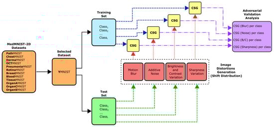
Figure 1.
Methodological framework for assessing data distribution shifts under image perturbations using the CSG metric. The proposed methodology is applied to the selected MedMNIST-2D dataset (YMNIST), with the corresponding parameters defined for each transformation in the “Image Distortions Generator”.
2.2. Dataset Complexity Measure
Computational efficiency is a pivotal consideration in data evaluation, especially for large-scale analyses. The Cumulative Spectral Gradient metric meets this need by providing a scalable, computationally efficient measure of multiclass classification complexity. Unlike conventional approaches that rely on expensive computations, CSG enables the rapid and accurate evaluation of dataset complexity. Its strong correlation with the generalization performance of CNNs makes it particularly valuable for model selection and hyperparameter optimization tasks.
The CSG metric is derived from the spectral analysis of an inter-sample similarity matrix. The matrix’s eigenvalue spectrum provides a quantitative measure of class separability. A dominance of low eigenvalues indicates well-separated, compact class clusters in the feature space, which corresponds to lower classification complexity. Conversely, a spectrum with elevated eigenvalues reflects significant overlap between classes, which directly correlates with increased classification difficulty. This spectral approach efficiently characterizes dataset complexity without requiring the computation of explicit class boundaries [12,23].
The CSG method starts with a nonlinear projection of the input data into a low-dimensional latent space. This optimizes the feature representation to align with the learning capacity of the model. Through this transformation, intra-class samples form compact clusters, and inter-class samples exhibit measurable separation. The divergence between class distributions ( and ) is quantified by computing the expected probability that M samples from one class will appear within the distribution of another class. This provides a robust measure of class separability (Equation (1)) [23,24]:
where represents M samples drawn from an identically and independently distributed class. This model is approximated using a K-nearest neighbor estimator according to Equation (2):
where is the number of neighbors around of class , M is the number of samples selected from class , and V is the volume of the hypercube surrounding the k samples closest to from class .
Next, the method computes the pairwise divergence between each class to construct a square similarity matrix, S, where quantifies the divergence between classes and . Each column vector of S subsequently serves as a class-specific signature. These signatures are then transformed into an adjacency matrix, W, through the Bray–Curtis distance, which establishes a weighted graph representation of inter-class relationships (see Equation (3)):
The weights of the adjacency matrix () quantify inter-class connectivity, with larger values indicating stronger relationships. Based on these weights, the following two calculations are performed:
- 1.
- Degree matrix D: A diagonal matrix in which each element represents the total connectivity of class i, and which is equal to the sum of the weights, , for each j.
- 2.
- Laplacian matrix : Encode the topological structure of class relationships.
The spectrum of the Laplacian matrix L comprises n eigenvalues, and the eigengap quantifies spectral discontinuities between consecutive eigenvalues. In this way, the dataset complexity metric integrates two spectral characteristics: (1) the area under the eigenvalue curve and (2) the normalized cumulative maximum of the eigengaps, weighted by , where K represents the number of classes [22,23]:
In any case, the two parameters that are configured for the implementation of the CSG algorithm are the number of samples (M) and the number of K-nearest neighbors (K). The first value corresponds to the number of representative samples selected from each class, and the second value corresponds to the number of nearest neighbors that are taken into account for each sample, which is essential for determining the separability of the classes. By evaluating the local neighborhood of each sample, the k-nearest neighbors approach provides information about class boundaries and improves the metric’s ability to capture the intrinsic complexity of the dataset. As stated in [23], the influence of the parameters K and M on the quality of the results is minimal, except in the particular case where M is very low. However, it should be noted that although the execution time is low, it varies almost linearly with M. Thus, the CSG method does not require careful adjustment of its hyperparameters. Consequently, the values of the parameters used in this research correspond to the default value of the number of samples (), and ten neighbors to calculate the likelihood distribution for each class (), in order to provide a balance between computational efficiency and the robustness of the results.
The CSG metric was evaluated by comparing its performance with that of classification models, specifically AlexNet, ResNet-50, and XceptionNet, both on binary datasets and on multiclass datasets (see [23] for more details). The comparison was made by analyzing the Pearson correlation and p-values of CSG with the performance of these models. The results of these tests allowed us to determine that the CSG metric is closely correlated with the generalization ability of Convolutional Neural Networks.
When evaluating a two-class dataset, the CSG metric ranges from 0 to 1, correlates well with CNN models, and is closely related to the complexity of the datasets. The results in two-class image classification problems achieved a Pearson correlation of 0.887 and a p-value of 0.113 with respect to the results when using an Xception model on four datasets (Inria, SeeFood, PulmoX, and the deer-dog subset of CIFAR10) [23]. In addition, the CSG value showed a gradual increase from the simplest dataset (Inria: CSG = 0.32, Xception error rate = 0.03), to intermediate values in slightly more complex datasets (deer-dog: CSG = 0.39, Xception error rate = 0.02, PulmoX: CSG = 0.55, Xception error rate = 0.11) approaching its maximum value in a more complex dataset (SeeFood: CSG = 0.95, Xception error rate = 0.21) [23]. Consequently, if the two classes are made up of original data (Class A) and distorted data (Class B) from the same class, the CSG metric will evaluate the level of complexity involved in separating data from the same class (adversarial validation between Class A and B). Thus, if the distorted data exhibits shifts in distribution with respect to the original data, i.e., statistically significant violations of the i.i.d. assumption, the CSG metric will tend toward 0, while if the modified data is not easily separable from the original data, the CSG metric will approach 1.
2.3. MedMNIST-2D
Although medical image analysis is critical for modern diagnostics, the development of robust machine learning models is often hindered by the complexity and heterogeneity of real-world datasets. To address this challenge, MedMNIST (Medical MNIST) was introduced as a lightweight yet comprehensive benchmark for 2D and 3D biomedical image classification. MedMNIST is designed to emulate the simplicity of the classic MNIST dataset while preserving the essential characteristics of medical imaging data. It provides standardized datasets spanning multiple imaging modalities, anatomical regions, and clinical tasks [25,26].
The MedMNIST collection includes twelve 2D image datasets (e.g., histology, X-rays, and dermatoscopy) and six 3D volume datasets (derived from CT scans), each of which is resized to a different resolution (from 28 × 28 to 224 × 224). The datasets are pre-processed from real-world sources such as the National Institutes of Health (NIH) ChestX-ray14 database, the ISIC Archive for Dermatology, and the LiTS Challenge for Abdominal CTs. This ensures clinical relevance while maintaining computational efficiency. MedMNIST provides predefined training and test splits to facilitate reproducible benchmarking of machine learning algorithms, from classical models to deep learning approaches [25].
Below, we provide an in-depth overview of the MedMNIST-2D datasets, covering their modalities, class distributions, and clinical applications. For the 3D datasets (e.g., OrganMNIST3D), please refer to the official MedMNIST publication ([25]). The description of the MedMNIST-2D datasets is divided into three groups: (1) binary classification with grayscale images (Table 1), (2) multiclass classification with grayscale images (Table 2), and (3) multiclass classification with color images (Table 3).

Table 1.
Characteristics of the MedMNIST-2D binary-classification datasets comprising grayscale images.
Table 2.
Characteristics of multiclass MedMNIST-2D datasets comprising grayscale images.
Table 3.
Characteristics of multiclass MedMNIST-2D datasets comprising color images.
These datasets cover a variety of diagnostic tasks, including detecting pneumonia in chest X-rays (PneumoniaMNIST), grading diabetic retinopathy (RetinaMNIST), and localizing abdominal organs in CT scans (OrganA/C/SMNIST). Despite their simplified resolution, the MedMNIST-2D datasets retain sufficient complexity to evaluate model generalizability. The datasets reflect clinical scenarios with class imbalances and imaging variations.
2.4. Distribution Shift
To simulate distribution shifts arising from real-world imaging variations, we implemented the following four clinically relevant distortion types: motion blur, additive noise, brightness/contrast (B/C) variation, and sharpness variation. These perturbations capture common disparities in medical imaging caused by devices and protocols. We applied the four distinct image perturbations systematically to simulate acquisition variations. Each parameter set was carefully selected to span clinically plausible ranges while maintaining anatomical interpretability.
- 1.
- Motion blur, which simulates patient movement during acquisition, is implemented via Gaussian kernel convolution with a radius of R pixels in the range of . This simulates increasing levels of patient movement while taking into account that motion artifacts degrade edge sharpness.
- 2.
- Additive noise, representing sensor or electronic degradation, is introduced by zero-mean Gaussian noise with standard deviations in to emulate the effects of sensor degradation, introducing stochastic signal corruption.
- 3.
- Brightness and contrast variation, which emulates exposure miscalibration, is achieved by adjusting both parameters simultaneously using the following pairs: . These pairs represent scanner exposure miscalibrations, where variations in illumination alter the perceived tissue contrast.
- 4.
- Sharpness variation used to adjust the sharpness of the image in order to modify image details and simulate artifacts that enhance the resolution of high-frequency details. Three values of enhancement factor were used: f in , where a value less than 1.0 gives a blurred image, a factor of 1.0 gives the original image, and a value greater than 1.0 gives a sharper image.
For each benchmark dataset, we generated 12 corrupted variants by systematically applying all combinations of four distortion types (motion blur, noise addition, brightness/contrast variation, and sharpness variation) across their respective parameter levels. We also generated a variant by comparing the original test data subset. This procedure yielded 996 perturbed datasets and 83 original classes (83 individual class variants × (12 corruptions + 1 original test set)). Figure 2, Figure 3 and Figure 4 illustrate representative examples of pristine and corrupted images across all datasets, demonstrating the visual impact of each distortion type.
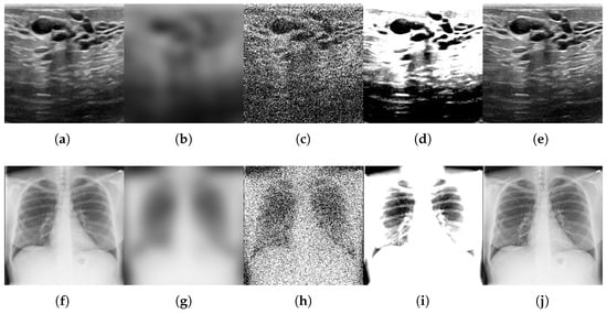
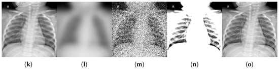
Figure 2.
Examples of original images and corrupted images with the four types of selected modifications, for the binary-classification MedMNIST-2D datasets comprising grayscale images: BreastMNIST, ChestMNIST, and PneumoniaMNIST. The maximum value of the parameter was taken for all types of distortions. (a,f,k) Original. (b,g,l) Blurred ( = 9). (c,h,m) Noisy ( = 90). (d,i,n) B/C variation (B = 0.6, C = 2.0). (e,j,o) Sharpened (factor = 2.8).
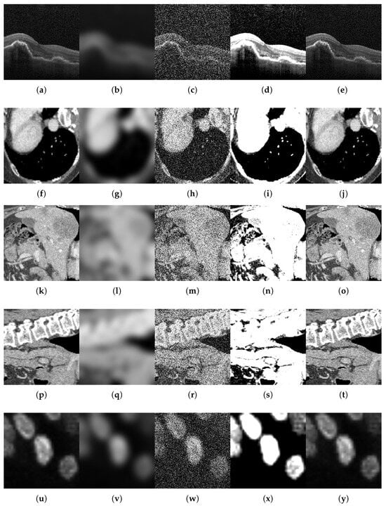
Figure 3.
Examples of original images and corrupted images with the four types of selected modifications, for the multiclass MedMNIST-2D datasets comprising grayscale images: OCTMNIST, OrganAMNIST, OrganCMNIST, OrganSMNIST, and TissueMNIST. The maximum value of the parameter was taken for all types of distortions. (a,f,k,p,u) Original. (b,g,l,q,v) Blurred (Radius = 9). (c,h,m,r,w) Noisy ( = 90). (d,i,n,s,x) B/C variation (B = 0.6, C = 2.0). (e,j,o,t,y) Sharpened (factor = 2.8).

Figure 4.
Examples of original images and corrupted images with the four types of selected modifications, for the multiclass MedMNIST-2D datasets comprising color images: BloodMNIST, DermaMNIST, PathMNIST, and RetinaMNIST. The maximum value of the parameter was taken for all types of distortions. (a,f,k,p) Original. (b,g,l,q) Blurred ( = 9). (c,h,m,r) Noisy ( = 90). (d,i,n,s) B/C variation (B = 0.6, C = 2.0). (e,j,o,t) Sharpened (factor = 2.8).
2.5. Adversarial Validation Analysis
We performed an experimental validation to quantify the distribution shifts between the corrupted test datasets and the original training data, using the CSG metric. We compared each perturbed test set variant to the training set, which served as the reference distribution. CSG scores provide a quantitative measure of distributional divergence; lower values indicate greater deviation from the reference distribution.
A systematic analysis of 1079 dataset comparisons revealed distinct distributional impacts for each distortion type. The CSG metric quantified the alterations in intra-class separability induced by distortion, demonstrating significant variations across perturbation categories.
3. Experimental Results
We present systematic evaluations of distribution shifts using the CSG score across four categories of perturbations: motion blur, additive noise, brightness/contrast variation, and sharpness variation. Each category is applied at three incremental intensity levels. This experimental design allows us to quantitatively assess how stronger distortions progressively affect the topology of the dataset and the distribution shift. The results are presented first for datasets that include grayscale images, then for datasets with color images, and finally a comparison of the proposed method against the results obtained with Cleanlab.
3.1. Adversarial Validation Results in Grayscale Images
The results of the proposed methodology applied to the MedMNIST-2D grayscale image datasets (binary and multiclass) are presented below. Figure 5 and Figure 6 present the CSG metric values computed between the training set and the corrupted test set variants. Class-specific measurements are shown for each distortion type and intensity level. This granular visualization enables two key analyses: (1) identification of class-specific vulnerability to different types of distortion, and (2) quantification of the effects of distortion severity across parameter values.
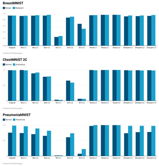
Figure 5.
Quantification of DS using the CSG metric, computed between each class in the training set and its corresponding class in: (1) the original test set, and (2) all corrupted test set variants. The CSG metric ranges from 0.0 (maximum DS) to 1.0 (minimum DS), with evaluations performed on the binary-classification MedMNIST-2D grayscale datasets (BreastMNIST, ChestMNIST, and PneumoniaMNIST). Corruptions include four modification types (motion blur, noise addition, brightness/contrast variation, and sharpness variation), each applied at three parameter levels.
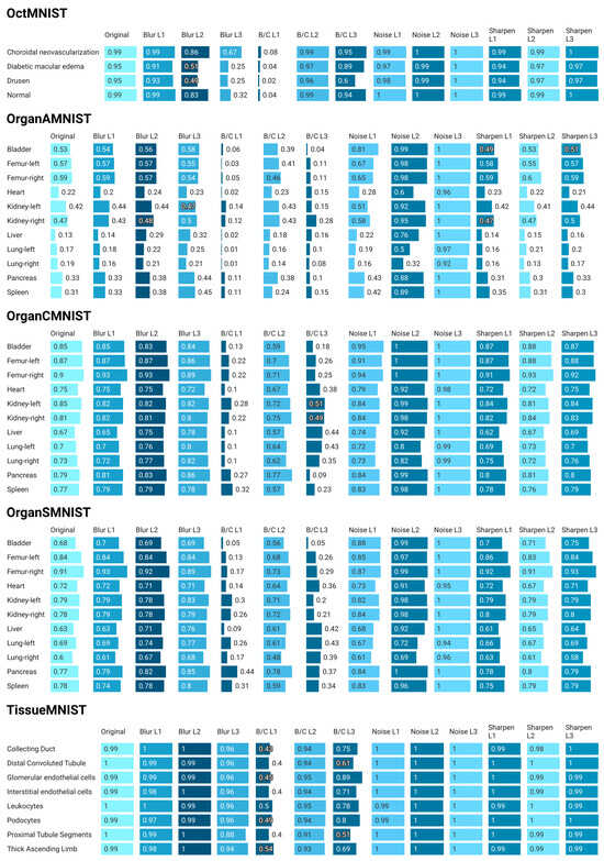
Figure 6.
Quantification of DS using the CSG metric, computed between each class in the training set and its corresponding class in: (1) the original test set, and (2) all corrupted test set variants. The CSG metric ranges from 0.0 (maximum DS) to 1.0 (minimum DS), with evaluations performed on the multiclass MedMNIST-2D grayscale datasets (OCTMNIST, OrganAMNIST, OrganCMNIST, OrganSMNIST and TissueMNIST). Corruptions include four modification types (motion blur, noise addition, brightness/contrast variation, and sharpness variation), each applied at three parameter levels. (The digital version of this figure offers greater visual clarity.)
According to Figure 5, the DS evaluated on BreastMNIST data is highly robust to blur, noise, and sharpening transformations. However, it is extremely sensitive to shifts in distribution introduced by changes in brightness and contrast, especially at the L1 and L3 levels. This poses a significant challenge for generalization in environments with varying illumination or image acquisition settings. Regarding ChestMNIST, the DS is reasonably vulnerable to blur and extremely sensitive to brightness and contrast shifts. These shifts cause a catastrophic increase in the DS, indicating a significant distribution shift that would hinder generalization in real-world scenarios with varying image acquisition settings. Regarding PneumoniaMNIST, the results are similar to those of ChestMNIST: the DS is robust against noise distortions and somewhat stable against focus distortions. However, it shows clear vulnerability to blur, especially for “normal” cases, and extreme sensitivity to brightness and contrast shifts, causing the DS to collapse. This indicates significant distribution displacement under brightness and contrast variations. The lower initial values for “normal” cases suggest that this class may be more challenging to characterize or more susceptible to subtle shifts.
As shown in Figure 6, OCTMNIST presents high robustness to noise and sharpening. However, it is quite sensitive to blur, especially for “Diabetic Macular Edema” and “Drusen”, and experiences extreme distribution displacement with brightness and contrast changes (i.e., a significant change in data distribution at certain levels). OrganAMNIST is the most challenging dataset yet with low baseline values for many classes. It exhibits extreme sensitivity to brightness and contrast shifts, resulting in near-total failure. Robustness to noise is not absolute for all classes, and the impact of blur and sharpening varies. This indicates a more complex interaction with distribution shifts and a reliance on different feature types per organ. OrganCMNIST shows high baseline values and robustness to noise and sharpening. It is more stable against blurring than OrganAMNIST but still experiences significant distribution shift due to changes in brightness and contrast. However, the impact may be less severe than in OrganAMNIST or OCTMNIST for the most extreme shifts. OrganSMNIST shows good robustness to noise and sharpening and moderate resilience to blurring. However, it consistently suffers from significant distribution displacement caused by brightness and contrast shifts, mirroring the vulnerability seen in other datasets. Finally, TissueMNIST is the most robust dataset among those shown in Figure 6. It demonstrates exceptional resilience to blur, noise, and sharpening. While brightness and contrast shifts cause a noticeable increase in DS, the impact is far less severe than in other medical imaging datasets. This suggests a lower degree of catastrophic distribution shift.
3.2. Adversarial Validation Results in Color Images
This section presents the results of the proposed methodology applied to the MedMNIST-2D color image datasets for multiclass classification, which are shown in Figure 7.
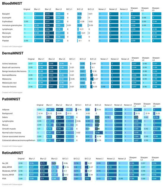
Figure 7.
Quantification of DS using the CSG metric, computed between each class in the training set and its corresponding class in: (1) the original test set, and (2) all corrupted test set variants. The CSG metric ranges from 0.0 (maximum DS) to 1.0 (minimum DS), with evaluations performed on the multiclass MedMNIST-2D color datasets (BloodMNIST, DermaMNIST, PathMNIST, and RetinaMNIST). Corruptions include four modification types (motion blur, noise addition, brightness/contrast variation, and sharpness variation), each applied at three parameter levels. (The digital version of this figure offers greater visual clarity).
Analysis of Figure 7 demonstrates that BloodMNIST models are highly robust to noise and sharpening. However, they are highly sensitive to blur and exhibit extreme vulnerability to brightness and contrast shifts. CSG values for most classes collapse entirely under these conditions. This suggests that variations in illumination or camera settings could render models trained on this data ineffective in real-world scenarios. DermaMNIST models are highly robust to blur, noise, and sharpening. However, they are extremely vulnerable to brightness and contrast shifts, mirroring the catastrophic failures observed in BloodMNIST and others. PathMNIST is characterized by class-dependent responses to transformations. It is extremely vulnerable to brightness and contrast shifts, which cause significant distribution displacement. Robustness to noise is generally high, while blur and sharpening effects are mixed and class specific. RetinaMNIST models are highly robust to noise and sharpening. However, they are moderately sensitive to blur and, critically, to brightness and contrast shifts, which cause considerable distribution displacement. The “PDR” class appears to be more robust to blur and brightness and contrast changes than other DR stages.
3.3. Overall Analysis
Across all 12 datasets, the CSG values remain consistently high (often approaching 1.0) when subjected to noise and sharpening transformations. This suggests that random pixel perturbations (noise) and edge enhancements (sharpening) generally do not induce significant shifts in the distributions that would alter the discriminative features within these diverse medical imaging modalities. Thus, models are inherently robust to these common image manipulations.
Regarding blurring, BreastMNIST and TissueMNIST demonstrate strong resilience, while ChestMNIST, PneumoniaMNIST, OCTMNIST, BloodMNIST, and RetinaMNIST show a noticeable or significant deterioration in distribution shift as blur increases. This suggests that preserving fine textural details and morphology is crucial for these tasks and that blurring introduces a relevant distribution shift. Conversely, OrganxMNIST and PathMNIST exhibit varied responses to blur. Some classes even demonstrate slight improvements at higher blur levels, suggesting a complex interplay between feature types and blur. Therefore, blur can induce a meaningful distribution shift depending on the dataset and the nature of the discriminative features (e.g., fine textures versus broad structures).
Brightness and contrast shift is the most critical and consistent finding across virtually all datasets. Brightness and contrast transformations produce catastrophic distribution shifts in BloodMNIST, DermaMNIST, ChestMNIST 2C, PneumoniaMNIST, OCTMNIST, and OrganAMNIST. BreastMNIST, PathMNIST, OrganCMNIST, OrganSMNIST, and RetinaMNIST experience substantial increases in distribution shift when brightness and contrast are altered. TissueMNIST is the only dataset that, while still impacted by brightness and contrast shifts, shows much greater resilience than all the others. Changes in brightness and contrast are the primary cause of severe distribution displacement across the spectrum of medical imaging tasks represented by these MNIST datasets. This strongly suggests that medical image analysis models depend heavily on specific pixel intensity distributions. Variations in illumination, camera settings, or scanner calibrations in real-world clinical environments pose the most significant threat to model generalization due to the profound shift in data distribution they induce.
3.4. Comparison of Results
In order to compare the results of the CSG metric as a tool for evaluating the distribution shifts in the used datasets, its application on test data was compared with the corresponding results obtained with Cleanlab [15]. The CSG metric was calculated on the five classes of RetinaMNIST, and its value was compared with the corresponding Non-IID scores of each class given by Cleanlab.
The data quality audit and detection of issues within the data and labels were performed using Datalab object, which facilitates the interface with the Cleanlab library. Here, we evaluate whether the overall dataset shows statistically significant violations of the IID assumption, such as change points or shifts, drift, autocorrelation, etc., all through the Non-IID score [27]. Although Cleanlab’s primary focus is at the sample level, the Non-IID score is actually a dataset-level check, not a per-data-point check (associated with whether the dataset violates the IID assumption or not). The Non-IID score ranges from 0 to 1.0 such that the lower the value, the greater the degree of violation of the IID assumption.
To detect Non-IID issues in the data using Cleanlab, an image classification model based on ResNet-50 pre-trained on ImageNet-1k was used [28,29]. K-fold cross-validation was used to train the ResNet-50 model in conjunction with early stopping to avoid overfitting. Next, the trained model was used to make predictions and obtain class probabilities, along with the features of the entire dataset. These probabilities and features were then used to inspect the dataset for potential problems using Datalab and Cleanlab.
The results of the distribution shift evaluation using Cleanlab’s Non-IID score and the CSG metric for each of the RetinaMNIST classes are shown in Figure 8.
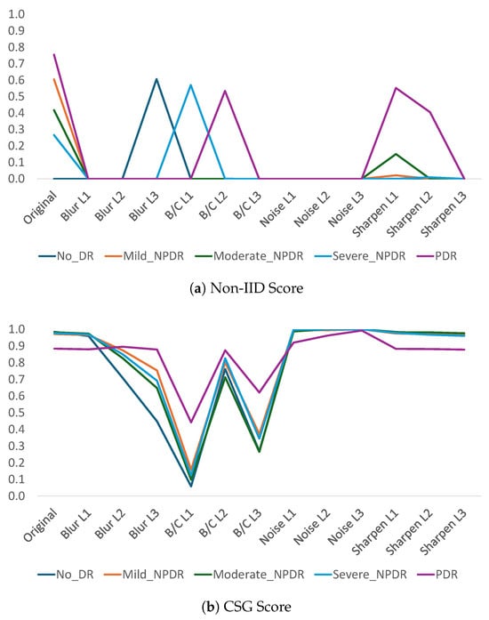
Figure 8.
Evaluation of distribution shift at the class level in RetinaMNIST for four types of image manipulation with three levels each, using two different metrics: Cleanlab’s Non-IID score and CSG score.
According to the results obtained with Cleanlab’s Non-IID score (Figure 8a and Figure 9), this metric tends to classify almost everything as a violation of the IID assumption. Even with the No-DR class of the original RetinaMNIST test data, the Non-IID score is zero. The only cases where the Non-IID score deviates from zero in the distorted data correspond to 10% of the 60 cases evaluated (5 classes × 4 types of distortion × 3 levels). These cases correspond to Blur L3-Class 0, B/C L1-Class 3, B/C L2-Class 4, sharpness L1-Class 2, sharpness L1-Class 4, and sharpness L2-Class 4. In any case, these cases are isolated since generally only one of the five classes exhibits this tendency. The fact that this metric generally yields values close to zero, combined with atypical behavior in some classes (contrary to the trend in the rest of the classes in the dataset), makes the non-IID score difficult to use in evaluating shifts in the data distribution.
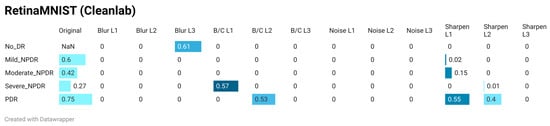
Figure 9.
Quantification of DS using the Non-IID score of Cleanlab, computed between each class in the training set and its corresponding class in: (1) the original test set, and (2) all corrupted test set variants. The Non-IID score ranges from 0.0 (maximum DS) to 1.0 (minimum DS), with evaluations performed on the multiclass RetinaMNIST 2D color dataset. Corruptions include four modification types (motion blur, noise addition, brightness/contrast variation, and sharpness variation), each applied at three parameter levels.
With regard to the results of the proposed method, the behavior shows that the metric tends to remain at 1, indicating that in most cases, even when distorted data is present, the complexity in the separability between the original and modified data remains high. It can also be seen in Figure 8b that the behavior of the metric is consistent across all classes such that the five classes show the same trend in terms of the CSG metric. That is, cases where the level of the metric is reduced (e.g., B/C L1 or B/C L3) show a reduction in the value of the metric for all classes, just as cases where high CSG values occur are found for all classes. Thus, the variability presented by the metric in Cleanlab for some isolated classes in blur, brightness and contrast, and sharpness modifications is also present in CSG but consistently for all classes.
Finally, a quantitative comparison is shown between the results of the CSG metric and the respective results when using Cleanlab’s Non-IID Score. Table 4 shows the results of the correlation coefficient between the CSG value vector of the five RetinaMNIST classes and the corresponding vector calculated using the Non-IID Score for each of the 13 perturbations (including the original).
Table 4.
Pearson correlation between the CSG measure and the Non-IID score across all perturbations, evaluated on the distribution shift results of the five RetinaMNIST classes.
According to the results in Table 4, there is a very strong negative linear relationship between the CSG metric values and the Non-IID Score per class for data with sharpness variation and data with added noise. In the case of results with brightness and contrast variations, the correlation is high for levels 2 and 3, and relatively low for level 1, in line with the variations shown in Figure 8. In the case of motion blur, the correlation is positive with intermediate values.
3.5. Discussion
The high sensitivity to variations in brightness and contrast in some MedMNIST datasets is due to the fact that medical pathologies are not defined by colors or global objects (as in natural image datasets such as ImageNet) but rather by subtle local textures and intensity gradients specific to each modality. Among the datasets most sensitive to brightness and contrast variations are those that rely almost exclusively on luminance to differentiate structures, such as OCTMNIST, OrganXMNIST, and those acquired by X-ray and ultrasound (ChestMNIST, PneumoniaMNIST, and BreastMNIST). In the case of OCTMNIST, this is because contrast is critical for distinguishing micrometric layers; when it is altered, pathologies such as macular edema may visually disappear. Abdominal organs, on the other hand, have very similar densities, so OrganXMNIST requires optimal contrast to prevent the edges between organs from becoming indistinguishable to a model. In images acquired using X-ray and ultrasound, increased brightness can whiten subtle pulmonary infiltrates, while low contrast makes it difficult to differentiate a tumor from normal dense tissue in breast ultrasounds.
As for RetinaMNIST or TissueMNIST, the impact is moderate to high, given that color and morphology help in these images, but brightness remains critical. In RetinaMNIST, for example, excessive brightness can hide very small dark spots representing micro-hemorrhages, causing false negatives in the detection of diabetic retinopathy. On the other hand, contrast variations in TissueMNIST images can alter the perception of the size and shape of cellular structures. In other texture- and color-sensitive datasets (e.g., BloodMNIST, PathMNIST, and DermaMNIST), lighting variations can alter saturation, making class separation difficult. For example, in DermaMNIST, a change in brightness can make a normal mole appear to be melanoma due to the alteration of pigment patterns.
It is also important to bear in mind that modalities such as Magnetic Resonance Imaging, digital histopathology, and retinography are subject to sources of noise such as magnetic field inhomogeneities, differences in staining protocols, and variations in lighting, which manifest as arbitrary changes in brightness and contrast. These inconsistencies degrade quantitative reproducibility and represent a critical obstacle to the development of robust artificial intelligence algorithms, as models can learn these acquisition artifacts instead of authentic morphological or functional biomarkers, hence the importance of using pre-processing techniques such as normalization, either with statistics-based methods (such as Z-score standardization) [30,31], bias field correction (e.g., N4ITK for MRI) [32], or color normalization in histopathology [33].
In terms of motion blur, the datasets most affected at level 3 are OCTMNIST and RetinaMNIST. In the first case, this is because when averaging neighboring pixels, the blurring merges the layers, eliminating a model’s ability to detect their thickness or separation, which are critical factors in identifying diseases such as macular edema. In the case of RetinaMNIST, blurring expands the brightness of small spots associated with micro-aneurysms and exudates, reducing their contrast and making them disappear visually against the background of the retina. In datasets such as OrganXMNIST, the impact may be moderate since, although blurring erases the edges of organs, the brightness of large organs such as the liver or lungs persists. In this way, a model may lose accuracy at the edges, but it can maintain some recognition ability based on location and overall size. On the other hand, datasets such as PathMNIST and DermaMNIST are less affected by motion blur-type variations since although Gaussian blurring eliminates surface details, the color stain and the overall structure of the lesion or stained cell are usually sufficient for the model to make a decision, being more resilient than purely radiological grayscale datasets.
Regarding the addition of Gaussian noise that alters pixel intensity values and consequently causes a significant distribution shift, it was found that the CSG metric fails to identify such shifts, except in datasets such as OrganXMNIST. In these datasets, different organs can have very similar densities on the grayscale, so Gaussian noise causes the pixels of one organ to shift to the intensity range of another, blurring anatomical boundaries. However, similar behavior was expected in datasets where the original signal-to-noise ratio is very low, such as PneumoniaMNIST, ChestMNIST, OCTMNIST, or TissueMNIST, where Gaussian noise easily obscures pathological signals. In these datasets, the CSG metric value remains close to 1 and fails to identify such shifts.
In order to complement the analysis of results with Interpretability techniques, training and inference were performed on a ResNet50-based model on which class activation maps were calculated. Interpretability in artificial intelligence is essential for understanding and explaining model predictions, a critical requirement for high-stakes applications [34]. Proposals for visual interpretability in deep learning have focused on methods derived from class activation mapping (CAM). Gradient-Weighted CAM (GradCAM) is a foundational technique that generates visual explanations by computing the gradients of a target class with respect to the activations of a final convolutional layer. Subsequent enhancements include GradCAM++, which employs higher-order gradients to better localize multiple or fine-grained object instances, and XGradCAM, which refines the method to improve two key properties: sensitivity (the correlation between feature removal and output change) and conservation (the faithfulness of the explanation’s magnitude to the model output) [35].
For the purpose of this study, a model based on the specified architecture was initialized with pre-trained weights from ImageNet1K-V1. The original classification head was replaced with a new layer tailored to the class count of the BloodMNIST dataset, and the final block of the network was unfrozen to enable fine-tuning. Training was conducted over 10 epochs using the Adam optimizer with a learning rate of 0.001 and cross-entropy loss. All experiments were performed on the Google Colaboratory platform utilizing an NVIDIA T4 GPU. Once the model was trained and adjusted, inference was performed on the original test image and the four distorted versions, and class activation maps were calculated using GradCAM++. The results are shown in Figure 10.
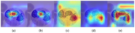
Figure 10.
GradCAM++ maps for a ResNET50 classification model, pre-trained on ImageNet and fine-tuned for BloodMNIST, calculated on a test image from the original dataset and its distorted versions. Regions of greatest relevance are highlighted in red, whereas lighter-colored areas indicate lower importance for the classifier. (a) Original. (b) Blurred ( = 9). (c) Noisy ( = 90). (d) B/C variation (B = 0.6, C = 2.0). (e) Sharpened (factor = 2.8).
The heat maps shown in Figure 10 highlight the specific parts of each image that the network focused on to classify the image. In this type of map, the regions of greatest interest correspond to red, while the areas in lighter colors have a lower degree of importance for the classifier. As can be seen, both the original image and the distorted images with blurring and sharpening coincide in the main region, which is consistent with the results analyzed so far. For its part, the location of the main area of interest in the heat map of the distorted image with B/C variation differs from the previous three, reflecting the degree of shift distribution in this type of modification. Finally, the heat map in the noisy image differs substantially from the other maps, and its most intense region also differs from the area identified in the original image. This in turn coincides with the previous analysis, related to the fact that the distribution shift in noisy images poses challenges for identification using the proposed methodology.
4. Conclusions
This study introduced a methodological framework for evaluating the impact of distribution shifts in medical datasets resulting from potential distortions during data acquisition. To support this analysis, the CSG score was employed as a measure of multiclass classification complexity associated with such shifts.
A systematic analysis of the diverse medical datasets undergoing various transformations provides a clear picture of distribution shifts. While these datasets generally exhibit remarkable robustness to common image corruptions, such as noise and sharpening, and varying sensitivity to blur, they consistently face critical, often catastrophic challenges from shifts in brightness and contrast.
This widespread vulnerability to brightness and contrast variations underscores a critical challenge in deploying medical image AI models in real-world settings, where such variations are prevalent. Based on the results of the research, it may be necessary to explore a broader set of parameter values or to adjust their values to reflect realistic clinical acquisition variability. For robust and reliable medical image analysis, future research must prioritize strategies that mitigate brightness and contrast-related distribution shifts. These strategies could include advanced data augmentation, domain adaptation techniques, or developing models that learn intensity-invariant features. Failing to address this vulnerability could severely undermine the clinical utility and reliability of these AI systems. As future work, other distortions related to the complex variability of real-world acquisition for specific capture types will be investigated, i.e., the impact on data distribution following the presence of modality-specific artifacts arising from the physics of medical imaging acquisition systems will be evaluated.
Author Contributions
Conceptualization, D.R.; Data curation, D.R.; Formal analysis, D.R., J.B. and E.M.-A.; Investigation, D.R.; Methodology, D.R.; Resources, D.R.; Supervision, D.R.; Validation, D.R., J.B. and E.M.-A.; Visualization, D.R., J.B. and E.M.-A.; Writing—original draft, D.R.; Writing—review and editing, D.R., J.B. and E.M.-A. All authors have read and agreed to the published version of the manuscript.
Funding
This work was funded by “Universidad Militar Nueva Granada-Vicerrectoría de Investigaciones” under the grant INV-ING-4157 of 2025.
Institutional Review Board Statement
Not applicable.
Informed Consent Statement
Not applicable.
Data Availability Statement
The image datasets used in this work are publicly available from MedMNIST [25], https://medmnist.com/ (accessed on 6 June 2025).
Acknowledgments
Diego Renza thanks the Universidad Militar Nueva Granada, since their contribution to this research is a product of the academic practice within this university. Jorge Brieva and Ernesto Moya-Albor thanks the Facultad de Ingeniería and the Institutional Program “Fondo Open Access” of the Vicerrectoría General de Investigación of the Universidad Panamericana for all their support in this work.
Conflicts of Interest
The authors declare no conflicts of interest.
Abbreviations
The following abbreviations are used in this manuscript:
| CT | Computed Tomography |
| CNN | Convolutional Neural Network |
| CSG | Cumulative Spectral Gradient |
| DS | Distribution Shift |
| i.i.d. | independent and identical distribution |
| ID | In-Distribution |
| ML | Machine Learning |
| MRI | Magnetic Resonance Imaging |
| NIH | National Institutes of Health |
| OOD | Out-Of-Distribution |
| PET | Positron Emission Tomography |
| US | Ultrasound |
References
- Clement David-Olawade, A.; Olawade, D.B.; Vanderbloemen, L.; Rotifa, O.B.; Fidelis, S.C.; Egbon, E.; Akpan, A.O.; Adeleke, S.; Ghose, A.; Boussios, S. AI-Driven Advances in Low-Dose Imaging and Enhancement—A Review. Diagnostics 2025, 15, 689. [Google Scholar]
- Abhisheka, B.; Biswas, S.K.; Purkayastha, B.; Das, D.; Escargueil, A. Recent trend in medical imaging modalities and their applications in disease diagnosis: A review. Multimed. Tools Appl. 2024, 83, 43035–43070. [Google Scholar]
- Melazzini, L.; Bortolotto, C.; Brizzi, L.; Achilli, M.; Basla, N.; D’Onorio De Meo, A.; Gerbasi, A.; Bottinelli, O.M.; Bellazzi, R.; Preda, L. AI for image quality and patient safety in CT and MRI. Eur. Radiol. Exp. 2025, 9, 28. [Google Scholar] [CrossRef]
- Bian, Y.; Li, J.; Ye, C.; Jia, X.; Yang, Q. Artificial intelligence in medical imaging: From task-specific models to large-scale foundation models. Chin. Med. J. 2025, 138, 651–663. [Google Scholar]
- Jiménez-Sánchez, A.; Avlona, N.; Boer, S.; Campello, V.; Feragen, A.; Ferrante, E.; Ganz, M.; Gichoya, J.; Gonzalez, C.; Groefsema, S.; et al. In the picture: Medical imaging datasets, artifacts, and their living review. In Proceedings of the 2025 ACM Conference on Fairness, Accountability, and Transparency (FAccT ’25), Athens, Greece, 23–26 June 2025; Association for Computing Machinery: New York, NY, USA, 2025; pp. 511–531. [Google Scholar]
- Daneshjou, R.; Vodrahalli, K.; Novoa, R.; Jenkins, M.; Liang, W.; Rotemberg, V.; Ko, J.; Swetter, S.; Bailey, E.; Gevaert, O.; et al. Disparities in dermatology AI performance on a diverse, curated clinical image set. Sci. Adv. 2022, 8, eabq6147. [Google Scholar] [CrossRef]
- Yao, H.; Choi, C.; Cao, B.; Lee, Y.; Koh, P.; Finn, C. Wild-time: A benchmark of in-the-wild distribution shift over time. In Proceedings of the 36th International Conference on Neural Information Processing Systems, New Orleans, LA, USA, 28 November–9 December 2022. [Google Scholar]
- Zhang, H.; Singh, H.; Ghassemi, M.; Joshi, S. “Why did the model fail?”: Attributing model performance changes to distribution shifts. In Proceedings of the 40th International Conference on Machine Learning, Honolulu, HI, USA, 23–29 July 2023. [Google Scholar]
- Kim, T.; Park, S.; Lim, S.; Jung, Y.; Muandet, K.; Song, K. Sufficient Invariant Learning for Distribution Shift. In Proceedings of the 2025 IEEE/CVF Conference on Computer Vision and Pattern Recognition (CVPR), Nashville, TN, USA, 11–15 June 2025; pp. 4958–4967. [Google Scholar]
- Taori, R.; Dave, A.; Shankar, V.; Carlini, N.; Recht, B.; Schmidt, L. Measuring robustness to natural distribution shifts in image classification. In Proceedings of the 34th International Conference on Neural Information Processing Systems, Vancouver, BC, Canada, 6–12 December 2020. [Google Scholar]
- Izzo, Z.; Ying, L.; Zou, J. How to learn when data reacts to your model: Performative gradient descent. In Proceedings of the 38th International Conference on Machine Learning, Online, 18–24 July 2021; pp. 4641–4650. [Google Scholar]
- Renza, D.; Moya-Albor, E.; Chavarro, A. Adversarial Validation in Image Classification Datasets by Means of Cumulative Spectral Gradient. Algorithms 2024, 17, 531. [Google Scholar] [CrossRef]
- Koh, P.; Sagawa, S.; Marklund, H.; Xie, S.; Zhang, M.; Balsubramani, A.; Hu, W.; Yasunaga, M.; Phillips, R.; Gao, I.; et al. WILDS: A benchmark of in-the-wild distribution shifts. In Proceedings of the 38th International Conference on Machine Learning, Online, 18–24 July 2021; pp. 5637–5664. [Google Scholar]
- Chen, A.; Lee, Y.; Setlur, A.; Levine, S.; Finn, C. Confidence-based model selection: When to take shortcuts for subpopulation shifts. arXiv 2023, arXiv:2306.11120. [Google Scholar] [CrossRef]
- Northcutt, C.; Jiang, L.; Chuang, I. Confident Learning: Estimating Uncertainty in Dataset Labels. J. Artif. Intell. Res. JAIR 2021, 70, 1373–1411. [Google Scholar]
- Yao, H.; Wang, Y.; Li, S.; Zhang, L.; Liang, W.; Zou, J.; Finn, C. Improving out-of-distribution robustness via selective augmentation. In Proceedings of the 39th International Conference on Machine Learning, Baltimore, MD, USA, 17–23 July 2022; pp. 25407–25437. [Google Scholar]
- Liang, W.; Yang, X.; Zou, J. Metashift: A dataset of datasets for evaluating contextual distribution shifts. arXiv 2022, arXiv:2202.06523. [Google Scholar] [CrossRef]
- Öztürk, Ş.; Duran, O.; Çukur, T. DenoMamba: A fused state-space model for low-dose CT denoising. IEEE J. Biomed. Health Inform. 2025. [Google Scholar] [CrossRef]
- Kabas, B.; Arslan, F.; Nezhad, V.; Ozturk, S.; Saritas, E.; Çukur, T. Physics-Driven Autoregressive State Space Models for Medical Image Reconstruction. arXiv 2025, arXiv:2412.09331. [Google Scholar]
- Zhang, S.; Zhang, X.; Shen, L.; Wan, S.; Ren, W. Wavelet-based physically guided normalization network for real-time traffic dehazing. Pattern Recognit. 2026, 172, 112451. [Google Scholar]
- Liu, Y.; Wang, X.; Hu, E.; Wang, A.; Shiri, B.; Lin, W. VNDHR: Variational Single Nighttime Image Dehazing for Enhancing Visibility in Intelligent Transportation Systems via Hybrid Regularization. IEEE Trans. Intell. Transp. Syst. 2025, 26, 10189–10203. [Google Scholar] [CrossRef]
- Aguilera-González, S.; Renza, D.; Moya-Albor, E. Evaluation of Dataset Distribution in Biomedical Image Classification Against Image Acquisition Distortions. In Proceedings of the 20th International Symposium on Medical Information Processing and Analysis (SIPAIM), Antigua, Guatemala, 13–15 November 2024; pp. 1–6. [Google Scholar]
- Branchaud-Charron, F.; Achkar, A.; Jodoin, P. Spectral Metric for Dataset Complexity Assessment. In Proceedings of the 2019 IEEE/CVF Conference on Computer Vision and Pattern Recognition (CVPR), Long Beach, CA, USA, 15–20 June 2019; pp. 3210–3219. [Google Scholar]
- González-Santoyo, C.; Renza, D.; Moya-Albor, E. Identifying and Mitigating Label Noise in Deep Learning for Image Classification. Technologies 2025, 13, 132. [Google Scholar] [CrossRef]
- Yang, J.; Shi, R.; Wei, D.; Liu, Z.; Zhao, L.; Ke, B.; Pfister, H.; Ni, B. MedMNIST v2-A large-scale lightweight benchmark for 2D and 3D biomedical image classification. Sci. Data 2023, 10, 41. [Google Scholar] [PubMed]
- Yang, J.; Shi, R.; Ni, B. MedMNIST Classification Decathlon: A Lightweight AutoML Benchmark for Medical Image Analysis. In Proceedings of the IEEE 18th International Symposium on Biomedical Imaging (ISBI), Nice, France, 13–16 April 2021; pp. 191–195. [Google Scholar]
- Cummings, J.; Snorrason, E.; Mueller, J. Detecting Dataset Drift and Non-IID Sampling via k-Nearest Neighbors. In Proceedings of the ICML 2023 Data-centric Machine Learning Research Workshop, Honolulu, HI, USA, 23–29 July 2023. [Google Scholar]
- Wightman, R.; Touvron, H.; Jégou, H. Resnet strikes back: An improved training procedure in timm. arXiv 2021, arXiv:2110.00476. [Google Scholar] [CrossRef]
- He, K.; Zhang, X.; Ren, S.; Sun, J. Deep Residual Learning for Image Recognition. In Proceedings of the 2016 IEEE Conference on Computer Vision and Pattern Recognition (CVPR), Las Vegas, NV, USA, 27–30 June 2016; pp. 770–778. [Google Scholar]
- Haga, A.; Takahashi, W.; Aoki, S.; Nawa, K.; Yamashita, H.; Abe, O.; Nakagawa, K. Standardization of imaging features for radiomics analysis. J. Med. Investig. 2019, 66, 35–37. [Google Scholar]
- Shinohara, R.; Sweeney, E.; Goldsmith, J.; Shiee, N.; Mateen, F.; Calabresi, P.; Jarso, S.; Pham, D.; Reich, D.; Crainiceanu, C.; et al. Statistical normalization techniques for magnetic resonance imaging. Neuroimage Clin. 2014, 6, 9–19. [Google Scholar]
- Kanakaraj, P.; Yao, T.; Cai, L.; Lee, H.; Newlin, N.; Kim, M.; Gao, C.; Pechman, K.; Archer, D.; Hohman, T.; et al. Deepn4: Learning N4ITK bias field correction for T1-weighted images. Neuroinformatics 2024, 22, 193–205. [Google Scholar] [PubMed]
- Xu, C.; Sun, Y.; Zhang, Y.; Liu, T.; Wang, X.; Hu, D.; Huang, S.; Li, J.; Zhang, F.; Li, G. Stain Normalization of Histopathological Images Based on Deep Learning: A Review. Diagnostics 2025, 15, 1032. [Google Scholar] [CrossRef] [PubMed]
- Bhati, D.; Neha, F.; Amiruzzaman, M. A Survey on Explainable Artificial Intelligence (XAI) Techniques for Visualizing Deep Learning Models in Medical Imaging. J. Imaging 2024, 10, 239. [Google Scholar] [CrossRef] [PubMed]
- Chavarro, A.; Renza, D.; Moya-Albor, E. ConvNext as a Basis for Interpretability in Coffee Leaf Rust Classification. Mathematics 2024, 12, 2668. [Google Scholar] [CrossRef]
Disclaimer/Publisher’s Note: The statements, opinions and data contained in all publications are solely those of the individual author(s) and contributor(s) and not of MDPI and/or the editor(s). MDPI and/or the editor(s) disclaim responsibility for any injury to people or property resulting from any ideas, methods, instructions or products referred to in the content. |
© 2026 by the authors. Licensee MDPI, Basel, Switzerland. This article is an open access article distributed under the terms and conditions of the Creative Commons Attribution (CC BY) license.