Abstract
This paper presents a novel data-driven approach to structural health monitoring (SHM) that uses Echo State Network (ESN) regression for continuous damage assessment. In contrast to traditional classification methods that demand extensive labeled data on damaged states, our approach utilizes an ESN, a powerful recurrent neural network, to directly predict a continuous damage metric from sensor data. This regression-based methodology offers two key advantages relevant to data science applications in SHM: (1) Reduced Training Data Dependency: The ESN achieves high accuracy even with limited data on damaged structures, significantly alleviating the data acquisition burden compared to classification-based AI/ML techniques. (2) Enhanced Noise Resilience: The inherent reservoir computing property of ESNs, characterized by a fixed, high-dimensional recurrent layer, makes them more tolerant of sensor noise and environmental variations compared to classification methods, leading to more reliable and robust SHM predictions from noisy data. A comprehensive evaluation demonstrates the effectiveness of the proposed ESN in identifying structural damage, highlighting its potential for practical application in data-driven SHM systems.
1. Introduction
Structural Health Monitoring (SHM) is paramount for ensuring the safety, longevity, and operational efficiency of civil infrastructure worldwide. Traditional SHM methodologies, often relying on periodic visual inspections or expensive, permanently installed sensor networks, present significant limitations in terms of cost, scalability, and continuous real-time assessment [1]. The pervasive availability and integrated sensing capabilities of modern smartphones offer a compelling opportunity to overcome these challenges by enabling ubiquitous, low-cost vibration monitoring. This paper introduces a novel regression-based SHM system using neural networks and smartphone to provide a continuous and nuanced assessment of structural integrity.
1.1. Traditional Structural Health Monitoring Methods
Historically, SHM has relied on several established methods, each with distinct characteristics:
Visual Inspection [2]: This is the most fundamental and widely used approach, involving manual assessment by trained experts to identify visible signs of damage such as cracks, corrosion, or deformation. While comprehensive for surface-level defects, visual inspection is inherently time-consuming, labor-intensive, costly for large structures, and highly subjective, relying heavily on the inspector’s experience. Crucially, it cannot detect internal or nascent damage that is not visually apparent.
Strain Gauges and Accelerometers (Direct Measurement) [3]: These sensors are directly affixed to structures to measure physical responses like stress, strain, and vibration. Strain gauges quantify deformation, while accelerometers measure dynamic acceleration responses. They offer quantitative and precise data, providing direct insights into structural behavior. However, their widespread deployment is often limited by intrusive installation requirements, high per-point costs, and the localized nature of their measurements, which may not capture global structural behavior or damage occurring between sensors. Maintenance and recalibration can also be significant challenges, hindering continuous, long-term monitoring.
Vibration-Based Techniques [4]: These methods analyze a structure’s dynamic response (e.g., natural frequencies, mode shapes, damping ratios) using specialized equipment and analytical methods such as modal analysis and random decrement techniques. The underlying principle is that changes in a structure’s physical properties due to damage will alter its dynamic characteristics. While effective for global damage detection, these techniques often require significant investment in high-fidelity instrumentation, complex data acquisition systems, and specialized expertise for data interpretation and model updating [5]. Furthermore, environmental and operational variations can significantly influence vibration characteristics, often masking or confounding damage-induced changes.
1.2. Classification-Based Data-Driven SHM Methodologies
The limitations of traditional methods have driven the development of more advanced SHM approaches, particularly those using data-driven techniques and machine learning [6]. Broadly, SHM methodologies can be categorized into approaches like computer vision [7], physics-based non-destructive testing (NDT) [8], and various machine learning-based and data-driven methods [9]. While computer vision and physics-based NDT offer powerful diagnostic capabilities, they often necessitate expensive and complex equipment, posing challenges for installation and sustained maintenance, thus limiting their suitability for continuous, long-term monitoring [5].
Consequently, a significant focus in modern SHM has shifted towards data-driven systems that frame the damage detection problem as a classification task [10]. These methods integrate modern signal processing techniques [11], advanced vibration analysis, and machine learning algorithms [12], including various neural networks [13], to achieve more efficient and accurate continuous structural monitoring [14]. Common classification algorithms employed include Support Vector Machines (SVMs), Artificial Neural Networks (ANNs), and Decision Trees, which are trained to distinguish between “healthy” and “damaged” states based on extracted features from sensor data.
However, a critical limitation of these classification-based techniques is their fundamental requirement for extensive labeled data representing both undamaged and various damaged structural states. Acquiring comprehensive and representative labeled data for a multitude of potential damage scenarios in real-world structures presents significant practical challenges, often being costly, time-consuming, and sometimes even impossible. This data scarcity can severely restrict the generalizability and robustness of classification models, especially for detecting unforeseen or novel damage types.
1.3. Regression-Based Data-Driven SHM Methodologies
To circumvent the challenges associated with labeled damage data in classification-based approaches, some researchers have explored reframing the SHM problem as a regression task. In these methodologies, the goal is to predict a continuous health index or damage severity level, rather than a discrete class. Regression-based SHM using neural networks has been demonstrated with various architectures, such as Long Short-Term Memory (LSTM) networks [15] and Convolutional Neural Networks (CNNs) [16]. These models are capable of learning complex nonlinear relationships within time series data to estimate damage severity.
Despite their strong performance in learning complex patterns, a significant drawback of these deep learning architectures (LSTMs, CNNs) is their high computational intensity. Deploying such models on resource-constrained devices like smartphones is often impractical due to limitations in processing power, memory, and battery life [9]. This computational burden can hinder their widespread adoption for real-time, on-device SHM applications.
1.4. Smartphone-Based Structural Health Monitoring
The ubiquity and affordability of smartphones, coupled with their increasingly sophisticated embedded sensors, have opened new avenues for cost-effective and readily deployable SHM solutions. Prior research has demonstrated the feasibility of using smartphone sensor data for structural damage identification across various contexts:
- (1)
- Vibration Monitoring: Data collected from smartphone accelerometers has successfully detected damage in building simulation testbeds [17], proving their capability to capture dynamic structural responses [18], such as bridge structural health monitoring [19].
- (2)
- Alternative Sensing Modalities: Beyond accelerometers, studies have explored monitoring magnetic field intensity variations with smartphones for detecting damage in steel plates through experimental and numerical studies [20], showcasing the versatility of smartphone sensors.
- (3)
- Wireless Sensor Networks: Wireless structural vibration monitoring systems based on Android smartphones have been designed and validated, achieving accurate time-synchronized monitoring by forming wireless sensor networks with multiple devices [21]. These systems often aim to diagnose building damage by aggregating data from interconnected devices [22].
- (4)
- Crowdsourcing & Multi-Sensor Systems: Community-based multi-sensor systems, leveraging diverse smart devices including smartphones and tablets equipped with cameras and vibration sensors [23], have also been explored for building damage monitoring, highlighting the potential for large-scale, distributed SHM networks [24].
While smartphone-based SHM offers unparalleled accessibility and cost-effectiveness, it also presents challenges [25]. These include the consumer-grade quality of embedded MEMS sensors (higher noise, lower precision compared to dedicated sensors), potential for inconsistent mounting, and battery life limitations for continuous operation. Despite these, the ongoing advancements in smartphone technology continue to enhance their viability for SHM applications.
1.5. Echo State Networks in Time Series Analysis and SHM
Echo State Networks (ESN) are a type of Recurrent Neural Network (RNN) based on the “reservoir computing” paradigm [26]. A key characteristic of ESNs is that only the weights connecting the reservoir to the output layer are trained, while the internal reservoir weights are fixed and randomly initialized. This significantly simplifies the training process compared to other RNN architectures, making them computationally efficient and less prone to vanishing/exploding gradient problems.
ESNs are particularly well-suited for processing complex time series data due to their inherent “echo state property,” which allows the reservoir to implicitly capture and retain a rich history of the input sequence. This makes them robust to noise and perturbations, a critical advantage when dealing with potentially noisy and variable sensor data, such as that acquired from smartphones. While ESNs have seen successful applications in various time series prediction tasks, their specific application to continuous damage metric regression in SHM, especially utilizing smartphone sensor data, remains an underexplored area. This work aims to bridge this gap by demonstrating the efficacy of ESNs for this novel SHM problem.
2. Data-Driven Structural Health Monitoring
In this paper, our Structural Health Monitoring (SHM) system is designed to detect damage that alters the fundamental dynamic properties of the monitored structure, specifically its stiffness and, to a lesser extent, its mass and damping characteristics. Such damage typically includes [1]:
- Stiffness Degradation: This is the most common type of damage detectable by vibration-based methods, resulting from phenomena like cracking, loosening of bolted or welded connections, or material degradation. A reduction in stiffness leads to changes in natural frequencies and mode shapes.
- Mass Changes: While less common for damage, unintended mass additions or losses could also be detected.
- Boundary Condition Changes: Alterations in how the structure is supported or restrained can significantly impact its dynamic response.
2.1. SHM Using Residual Distance Method
The Residual Relative Error (RRE) calculates the relative error in the residual sequences at each sensor for different structural conditions, in vector case
where, and represent the n-dimensional residual vectors corresponding to the undamaged and damaged states, respectively [27]. represents the norm.
By utilizing the residual vectors of all sensors under damaged and undamaged conditions, it is possible to construct a vector containing the quantities in the following manner:
where represents the number of sensors. During a test measurement, RRE consists of elements, where each element corresponds to the RRE value at a specific sensor. In the presence of structural damage, the residual samples tend to increase, allowing the RRE index to effectively identify and detect the damage. The Mahalanobis squared distance is a widely recognized and robust statistical metric used to quantify the similarity between two multivariate datasets. This method is scale and amount invariant, computing similarity based on the correlation between variables.
Let represent a multivariate feature matrix obtained from the undamaged (healthy) state, where is the number of data rows (observations). From this healthy reference data, we compute the mean vector and the covariance matrix where is invertible and For any new observation vector which is a row vector from a test dataset the MSD calculates its distance from the healthy reference distribution as follows:
For a set of new observations the vector of Mahalanobis squared distances are given by:
Here, represents the distance of the dataset Z from the reference dataset X, which can be effectively utilized to calculate the statistical distance between time series data from damaged and non-damaged structural conditions [28]. A significant increase in values for a new measurement, compared to the baseline, indicates a deviation from the healthy state, signaling potential damage.
2.2. Pre-Processing and Analyzing Vibration Data
We have four smartphones at our disposal for data collection, enabling us to record accelerations on each floor of the building along the X, Y, and Z axes, as shown in Figure 1. The earthquake’s vibration is simulated by the acceleration of the XY-axis motor at the bottom. Since the start times of different phones may vary, we utilize Dynamic Time Warping (DTW) [29] to synchronize the start times. In the case where we have two time series,
where n and m represent the lengths of time series G and H.

Figure 1.
Platform of SHM system.
The DTW algorithm consists of three main stages:
(1) Local Distance Matrix Population: In the first stage, a local distance matrix d is constructed. Each element in this matrix is populated with the Euclidean distance (or another suitable distance metric) calculated between each pair of points from time series G and from time series H. That is,
(2) Warping Matrix Computation: In the second stage, a cumulative cost matrix, referred to as the warping matrix D, is filled based on the DTW recurrence relation:
This matrix, having the same dimensions as the local distance matrix, represents the minimum accumulated distance to align the prefix of G up to with the prefix of H up to .
(3) Optimal Warping Path and DTW Distance Calculation: Finally, the optimal warping path W is determined by backtracking through the warping matrix D from to , following the path of minimum accumulated cost. The warping path is a sequence of adjacent matrix elements:
where k is the total number of elements in the warping path. represents a pair of indices from G and H, respectively, This path establishes the nonlinear mapping between G and H that minimizes their overall alignment distance. The warping path inherently possesses three critical attributes, guaranteeing its validity:
(1) Monotonicity: Any two adjacent elements of the warping path: and , the indices must not decrease, i.e., and This ensures that the alignment progresses forward in time for both series.
(2) Continuity: For any two adjacent elements of the warping path: and , the indices can only advance by at most one step, i.e., and This prevents skipping points in the alignment.
(3) Boundary: The warping path must start from the first elements of both time series, , and end at their last elements, . The warping path starts from the top left corner and ends at the bottom right corner.
The DTW distance between the two time series, , is the cumulative distance along this optimal warping path, which is given by the value from the warping matrix. To enable comparison between alignments of time series with potentially different lengths or path complexities, this cumulative distance is commonly normalized by the length of the warping path K:
Furthermore, to improve identification accuracy, an additional step was taken to implement a low-pass filter (LPF) [30]. The LPF is defined by the following discrete difference equation:
In the context of digital signal processing, x denotes the signal subject to filtration. represents the signal value before the application of the low-pass filter, while represents the signal value after the low-pass filter has been applied. denotes the cutoff frequency of the low-pass filter, and T indicates the total number of iterations when the low-pass filter is employed.
The SHM system comprises three steps. In the first step, we utilize DTW to align the time axis and ensure consistent start times. The second step involves the use of discrete low-pass filtering to enhance signal discrimination. The third step entails utilizing the echo state network to model the damaged and undamaged structures separately. Furthermore, the subsequent section provides a description of the robust echo state network under discussion.
The proposed method includes the following parts:
- Data Collection: It is the process of collecting data from smartphones using the developed application. This includes sensor selection, calibration procedures (if any), and data recording protocols. If using real-world structures, describe the selection criteria for the structures and how damage conditions were assessed.
- Data Preprocessing: We use methods to clean and prepare the collected sensor data for neural network training. This involve filtering techniques to remove noise, normalization of data values, and potentially feature engineering to extract relevant features from the raw sensor data.
- Neural Network Model Design: We use ESN for regression. The number of neurons, activation functions, and relevant hyperparameters will be discussed in the next session. The training process for the ESN model, including the training data used, the chosen optimizer algorithm, and the loss function used to evaluate model performance during training will also be discussed.
3. Echo State Network Regression for SHM
In this paper, we use the ground-based data [1], which are taken from sensors placed on the ground or foundation of a structure. This data represents the input excitation to the structure. This data is used as input for the network, with damaged or undamaged data serving as the target for training.
This section initially addresses the reduction in classification problems to regression problems. It then introduces a proposal for a robust echo state network.
3.1. Problem Definition
Linear Classification [31]: We assume that the training data consists of N data set , D is the dimension of the feature space . Each data set has a unique true label . The objective function for the loss linear classification problem can be defined as . Here, w is solved by . This problem has been shown to be NP-hard [32].
Linear Regression [31]: The objective function can be defined as , where y represents the vibration time series, w is solved by . Solving this problem has an efficient analytic solution, which is easier than linear classification.
Our primary focus is continuous damage assessment via regression, it is theoretically possible to derive a classification decision from the regression output by applying a threshold. In such cases, a low regression error can provide a bound for the 0-1 classification error, implying that . This suggests that robust regression performance can indirectly support effective classification,
where represents the out-of-sample error, represents the in-sample error, N represents the size of the training set.
represents the Vapnik Chervonenkis (VC) dimension [31] of the classification model . VC dimension is a measure of the capacity or complexity of a machine learning model. It indicates the maximum number of points that the model can classify in all possible ways. A higher VC dimension generally implies a more complex model with a greater capacity to fit data, but also a higher risk of overfitting.
The following lemma asserts that the regression method is capable of completing the classification task.
Lemma 1
([31]). In binary classification, given function class F with Vapnik Chervonenkis (VC) dimension , we have the following risk bound for any classifier . When and , the bound holds with probability at least .
In the field of structural health monitoring procedures, there is a scarcity of labeled data, particularly for damaged instances. This limitation hampers efforts to diminish the out-of-sample error, . Moreover, achieving a favorable value for proves challenging due to its association with NP problem and its consequent tight bounds. Our objective is to employ regression for classification tasks, placing emphasis on efficiency rather than strict boundary adherence. In (9), we can also observe that as long as the regression is done well, the classification effect can also be achieved.
3.2. Echo State Network
The mathematical expression of ESN is
where the input to the ESN at time step t is denoted by , where n is the dimensionality of the input. The output of the network at time step t is denoted by , where m is the dimensionality of the output. The state of the reservoir layer at time step t is given by . The ESN has a reservoir layer consisting of N neurons, is the input weight matrix, is the recurrent weight matrix, is the output weight matrix, and is an element-wise activation function.
The recurrent layer is
where is the leaking rate. The weights and are randomly initialized with fixed weights.
In batch cases, the weights of the output layer are adjusted using the least squares algorithm
where X is the matrix of reservoir states for all time steps t, Y is the matrix of desired outputs for all time steps t, is a regularization parameter, and I is the identity matrix. For time series modeling, Y is the target vector, X is historical data. This approach greatly simplifies the training process and reduces the risk of overfitting, since the complexity of the model is largely determined by the size and connectivity of the reservoir layer.
The hyperparameter selection methods include grid search, random search, and evolutionary algorithm, provided the ranges or discrete values explored for each key hyperparameter. The output weights obtained from the training process will be applied for structural health monitoring, as depicted in Figure 2.
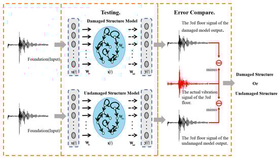
Figure 2.
Smartphone-based SHM.
3.3. Training of Echo State Network
The main focus of this section is to discuss the challenge in selecting an appropriate learning rate to ensure fast learning during the process of gradient descent. Consider following a discrete-time state-space nonlinear system.
In the given equation, represents the input vector, denotes the state vector, and f represents a general, nonlinear, smooth function.
The identified nonlinear system, denoted as Equation (14), is bounded-input and bounded-output (BIBO) stable, with both and being bounded. Utilizing the Stone–Weierstrass theorem, this nonlinear system can be expressed as follows:
From (14), (15) and (16)
The training process of the smartphone-based SHM is shown in Figure 3.
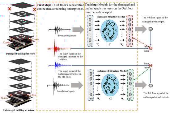
Figure 3.
Training phase of the smartphone-based SHM.
Theorem 1.
Suppose the neural network (14) is utilized for identifying a nonlinear plant. If α is chosen such that , applying the following gradient updating law with a robust modification ensures the boundedness of the identification error .
where satisfies
The proof is shown in the Appendix A.
4. Experimental Results
4.1. Smartphone-Based SHM Platform
The proposed Structural Health Monitoring (SHM) platform uses readily available and affordable smartphones as sensing units. The main parts of this platform are:
- Smartphones: iPhone X devices were used as the main data collection tools because they have good built-in accelerometers that work well.
- Sensors: iPhone X has tri-axial accelerometers inside, which were used to measure how the structure moved in three directions (X, Y, and Z).
- Data Acquisition App: A special app we created was used to get the raw accelerometer data. The app was set to record data 100 times per second for 90 s each time.
- Computing Platform: A computer with Windows 10 was used to manage communication with the smartphones, process and analyze the data, and run the trained ESN to find damage (as shown in Figure 4).
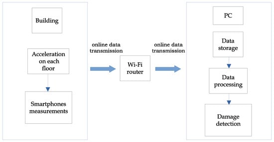 Figure 4. Functioning blocks of the smartphone-based SHM system.
 - Two-floor laboratory-scale structure: It is specifically designed for controlled experimental validation and constructed entirely from aluminum. It stands 100 cm in height, with a width of 40 cm and a depth of 30 cm. This choice of material and a simplified, yet dynamically representative, configuration allows for precise control over damage induction and ensures repeatable experimental conditions, which would be prohibitively expensive and logistically challenging with full-scale structures. By detailing these exact specifications, we aim to provide complete transparency regarding our experimental setup, enabling other researchers to accurately assess the context and implications of our results for broader Structural Health Monitoring applications.
Smartphones have sensors inside, don not cost a lot, and are easy to move around to collect data. We used both iOS (iPhone X) and Android phones, because they are partly open-source, and there are tools that let you directly access the sensors like accelerometers and gyroscopes. The data from these sensors was accessed using the phone’s built-in sensor management system at regular times. The overall design of our SHM system is shown in Figure 5.
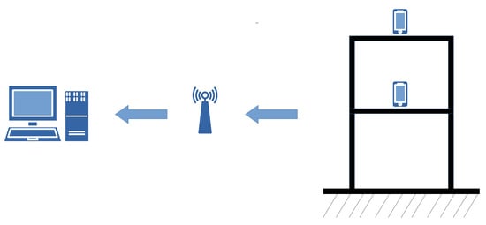
Figure 5.
Scheme of smartphone-based SHM system.
Modern smartphones contain Micro-Electro-Mechanical Systems (MEMS) accelerometers that measure proper acceleration along three axes. Their typical specifications are: sampling rates are 100–200 Hz, dynamic ranges are ±2 g to ±16 g. Their key advantages are: low cost, ubiquity, and ease of deployment. Their limitations are: higher noise compared to research-grade sensors, potential for drift, and power constraints for long-term monitoring.
The smartphones, serving as our vibration sensors, were placed on the foundation (ground level) and the center of each floor level of the multi-storey test structure. These devices are positioned flat on the floor surface, with their X-axis and Y-axis aligned perpendicular to the directions of excitation, and their Z-axis (vertical) aligned with the gravitational direction.
4.2. Detection of Structural Damage Through Vibration Amplitude Changes
The dynamic behavior of a structure is characterized by key vibration properties. Natural Frequencies, intrinsic to a structure’s stiffness and mass, decrease with damage. Mode Shapes, the spatial deformation patterns, also change as damage alters stiffness distribution. Damping Ratios, representing energy dissipation, can increase or decrease due to damage, such as loosened connections. Amplitude/Displacement/Acceleration quantify vibration magnitude; under consistent excitation, altered magnitudes can signify damage. This paper specifically utilizes changes in the amplitude/displacement/acceleration time series within our regression-based approach to infer structural health.
To facilitate a comparison between structurally damaged and undamaged data, we aligned measurements obtained from both scenarios using a time-synchronization algorithm. This ensured a coherent time frame for both sets of measurements. The destructive methodology involved removing two screws from the base, simulating structural damage.
After aligning the data, a comparison was made between the two sets of measurements, as illustrated in Figure 6. As an illustrative example of a damage-sensitive vibration characteristic, we observed that when the structure is damaged, there is a notable increase in vibration amplitude along the Y-axis. This specific change is attributed to the altered force transmission paths within the damaged structure, causing energy to redistribute from the X-axis to the Y-axis and Z-axis. Consequently, for this particular structural configuration, the amplitude of the Y-axis effectively serves as a criterion for assessing structural damage.
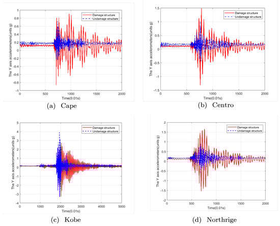
Figure 6.
Vibrations along the Y-axis for both undamaged and damaged structures during four types of earthquakes.
In this experiment, we will use the discrepancy between the predicted output of ESN and the actual output of the damaged or undamaged structure as a metric to determine the extent of structural damage. When the error generated by the damaged model (where ESN train data consists of damaged structure vibration data) was low, the corresponding structure was classified as damaged. Conversely, when the error generated by the undamaged model (where ESN train data consists of undamaged structure vibration data) was low, the structure was considered healthy. The ESN was trained using the house’s foundation signal as input, with sensor signals recorded both before and after structural damage serving as the corresponding output.
4.3. Echo State Network for Structural Health Monitoring
In this experiment, we used the discrepancy between the predicted output of ESN and the actual output of the damaged or undamaged structure as a metric to determine the extent of structural damage. When the error generated by the damaged model (where ESN train data consists of damaged structure vibration data) was low, the corresponding structure was classified as damaged. Conversely, when the error generated by the undamaged model (where ESN train data consists of undamaged structure vibration data) was low, the structure was considered healthy. The house’s foundation signal served as the input to the ESN, with sensor signals before and after structural damage as the corresponding output signals.
Subsequently, tests were conducted on the foundation vibration data collected in Cape, keeping the previously learned parameters of the RESN fixed. The network exhibited high sensitivity to abrupt changes in the data due to damages in the building structure.
4.4. Experimental Results
In our study, we used iPhone X devices, and their battery life was long enough for our 90-s recordings. To start each test, an iPhone X was placed securely on the test bench. Before recording, we did a zeroing process by averaging the accelerometer readings for 20 s while the phone was still. This gave us the baseline readings when there was no movement (0 g): V (x-axis), V (y-axis), and V (z-axis). After zeroing, we recorded acceleration data for 90 s at a rate of 100 samples per second, which gave us 9000 data points for each direction.
In this paper, we use the ground motion records of the Kobe (1995), Northridge (1994), El Centro (1940), and Cape Mendocino (1992) earthquakes, which are obtained from the Pacific Earthquake Engineering Research (PEER) Center’s NGA-West2 Database [33]. We did these simulations while the iPhone X devices recorded how the structure moved at the places where they were attached. To prepare the training dataset we use the following steps:
- (1)
- Raw Data Acquisition: We reiterate that the raw acceleration data was collected from smartphone accelerometers strategically positioned on the structure’s foundation and various floor levels at the dedicated test station.
- (2)
- Data Synchronization: We use Dynamic Time Warping for the time series from different sensors were synchronized to a common timeline. As previously discussed, Dynamic Time Warping was employed to align these series, accounting for inherent nonlinear phase differences in structural responses.
- (3)
- Preprocessing: We applied a low-pass Butterworth filter with a cutoff frequency 20 Hz to remove high-frequency noise and focus on the relevant structural vibration frequencies. To ensure consistent input scales for the ESN and prevent features with larger magnitudes from dominating, the filtered data was normalized using a Min-Max scaling across the entire dataset.
- (4)
- Input–Output Pair Formation:The preprocessed acceleration data from the foundation sensor served as the input to the ESN. The corresponding output (target for regression) was the derived damage metric or health index for that specific structural state (healthy or damaged), as determined by the controlled experimental conditions.
We use the following NMSE (Normalized Mean Square Error) as the experimental error. This is used metric to evaluate the performance of regression models. A lower NMSE indicates better predictive accuracy.
where y is the network output, and is the expected output.
It stands for normalized mean squared error, a widely used metric for evaluating the performance of predictive models. It is a normalized version of the mean squared error (MSE) and is calculated by dividing the MSE by the variance of the target variable. NMSE provides a normalized measure of the prediction error, useful for comparing models with different units or scales.
As shown in Figure 3, with the selection of an appropriate model, a low error rate and accurate fitting of the Cape vibration data were achieved. These experiments provide compelling evidence that structural failures of the same type can be successfully modeled. Using Cape earthquake data, Figure 7 illustrates that the output generated by the model aligns with the vibration generated by the actual structure, enabling the detection of structural damage. For Northridge earthquakes, detection of building damage was possible, as depicted in Figure 8, where the prediction errors are displayed.
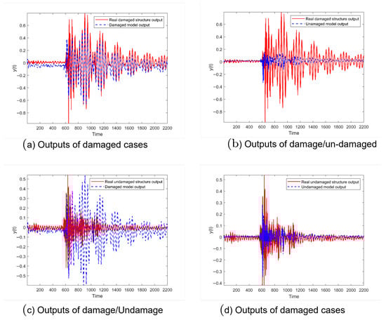
Figure 7.
Detection phase of structural damage using Cape earthquake data.
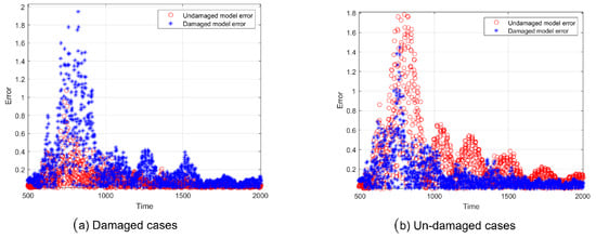
Figure 8.
The prediction errors corresponding to the damaged and undamaged structure models using Northridge earthquake data.
Table 1 displays NMSE values obtained from the ESN model for various earthquake types. In this context, ‘Damaged’ refers to buildings with structural damage, while ‘Undamaged’ denotes intact buildings. “” represents the modeling error of the neural network for damaged building structures, and “” represents the modeling error for undamaged building structures.

Table 1.
ESN regression for arious earthquakes.
The results indicate the successful detection of damage by the ESN model across all earthquake types. The ESN demonstrated accurate modeling for both damaged and undamaged cases. In the damaged scenario, the modeling error “” for damaged building structures was significantly lower than that for undamaged structures (“”), implying structural damage. Conversely, in the undamaged scenario, the modeling error “” for undamaged building structures was notably lower than that for damaged structures (“”), indicating an undamaged structure. Therefore, the ESN model effectively detects damage across different earthquake types and differentiates between damaged and undamaged structures.
To assess the performance of our newly proposed ESN, we compare it with Multilayer Perceptrons (MLP) and Radial Basis Function (RBF). Table 2 and Table 3 reveal that MLP and RBF perform well in detecting damaged structures but struggle to effectively detect undamaged structures, potentially leading to misjudgment. The Echo State Network presents a promising solution for detecting structural damage in building sensor data, outperforming MLP and RBF in terms of accuracy and robustness.
Table 2.
MLP regression for various earthquakes.
Table 3.
RBF regression for various earthquakes.
4.5. Discussions
The demonstrated efficacy of ESN approach in regressing structural health from vibration data, particularly when utilizing lower-fidelity sensors like smartphones, underscores its significant potential for advancing cost-effective and accessible Structural Health Monitoring. Our regression-based method provides a continuous damage metric, offering a more nuanced assessment than binary classification, its current implementation relies on supervised training with labeled data for both healthy and damaged structural states, see Figure 9. This approach allows the ESN to learn the intricate relationship between vibration patterns and varying degrees of structural integrity. This capability broadens the scope of SHM applications, making continuous structural assessment more feasible for a wider range of infrastructure.
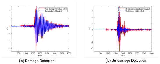
Figure 9.
Training phase for damage detection using echo state networks with Kobe earthquake data.
Building on these promising results, several key avenues for future research are identified to further enhance the robustness, comprehensiveness, and applicability of the ESN-based SHM system:
- Multi-Sensor Data Fusion: Investigate the synergistic integration of data from other readily available smartphone sensors, such as gyroscopes for capturing rotational dynamics and magnetometers for potential insights into the integrity of steel components. Fusing these diverse data streams could provide a more comprehensive understanding of complex structural behaviors and damage mechanisms.
- Environmental Factor Integration: Explore the incorporation of environmental data, including temperature, humidity, wind speed, and barometric pressure, into the ESN regression models. This integration is crucial for improving the robustness and accuracy of damage assessment by explicitly accounting for external factors that influence structural response and sensor readings, thereby minimizing false positives.
- Real-time Anomaly Detection: Develop and implement real-time damage detection capabilities by integrating anomaly detection algorithms with the ESN regression framework. This would enable continuous, automated monitoring and immediate identification of deviations from normal structural behavior, facilitating early intervention and preventive maintenance.
- Transfer Learning for Adaptability: Investigate the application of transfer learning techniques to expedite and enhance the training of ESN models for specific damage types or when adapting the system to new structural characteristics. Leveraging pre-trained reservoir states or fine-tuning model weights could significantly reduce the need for extensive new baseline data collection across diverse buildings or damage scenarios.
- Cloud-Based Computational Offloading: Explore the feasibility and benefits of offloading computationally intensive aspects of ESN training and real-time analysis to cloud-based platforms. This strategy would enable the deployment of more complex models and the efficient processing of large-scale data streams from numerous distributed smartphone sensors, paving the way for scalable urban SHM networks.
The proposed regression-based SHM system, with its focus on accessible sensing and efficient learning, holds significant potential for a wide range of practical applications in civil engineering and infrastructure management:
- Integration with Building Information Modeling (BIM): Seamlessly integrate the SHM system with BIM platforms to create a comprehensive structural health management ecosystem. This integration would provide real-time performance data, enabling informed decision-making regarding maintenance scheduling, repair strategies, and long-term lifecycle management of assets.
- Data-Driven Predictive Maintenance: Enable proactive and data-driven predictive maintenance strategies for buildings by continuously monitoring their structural health. This approach allows for the early identification of potential issues before they escalate into critical failures, thereby reducing costly emergency repairs and minimizing operational downtime.
- Crowd-Sourced Urban SHM Networks: Facilitate the development of large-scale, crowd-sourced SHM networks by leveraging the ubiquitous smartphones of building occupants. This innovative approach offers a highly cost-effective and scalable solution for continuously monitoring the health of a vast number of urban structures, contributing to enhanced urban resilience and safety.
5. Conclusions
This paper introduces a novel and specifically tailored Echo State Network regression framework for continuous structural health monitoring, effectively addressing key limitations inherent in traditional classification-based methods. By directly predicting a continuous damage metric from sensor data, our approach circumvents the need for extensive labeled datasets on damaged structural states. The inherent architecture of the ESN facilitated efficient training, even with limited data representing damaged conditions, thereby significantly reducing the data acquisition burden often associated with classification techniques. Moreover, the ESN’s reservoir computing properties demonstrated enhanced resilience to sensor noise and environmental variations, leading to more reliable and robust damage assessments.
Our ESN approach aims to maximize utility even from lower-fidelity data, potentially enhancing the feasibility of using more accessible, lower-cost sensors in SHM. Future research will focus on expanding the applicability of this ESN regression framework to a wider range of structural types and operational conditions. Further investigations will also explore refinements to the ESN architecture, including optimization of reservoir parameters and the incorporation of attention mechanisms, to achieve even greater accuracy, robustness, and interpretability in continuous structural health monitoring.
Author Contributions
Methodology, X.L., W.Y. and Y.Z.; Software, Y.Z.; Writing original draft, X.L. and W.Y.; Writing review & editing, X.L. and W.Y. All authors have read and agreed to the published version of the manuscript.
Funding
This work was supported by Mexican CONAHCYT (Consejo Nacional de Humanidades, Ciencias y Tecnologias) under the grant CF-2023-I-2614.
Institutional Review Board Statement
Not applicable.
Informed Consent Statement
Not applicable.
Data Availability Statement
The data presented in this study are openly available in the link in reference [33].
Acknowledgments
We would like to thank Carlos Parga for providing smartphone interface with PC.
Conflicts of Interest
The authors declare no conflicts of interest regarding the publication of this article.
Appendix A
Proof of Theorem 1.
To find the required stability conditions, We select Lyapunov funvtion as
Based on the Lyapunov stability theory, if a positive definite function and its time derivative hold for the error dynamics of a neural network, then i.e., the output tracking error
Now we need to prove that Because
There exist a constant , such that
(a) if ,
where , .
Finally,
When
then So
(b) If the condition is satisfied, then , which implies that is constant, as well as . Since , we can conclude that is bounded. □
References
- Balageas, D.; Fritzen, C.-P.; Güemes, A. Structural Health Monitoring; Wiley: Hoboken, NJ, USA, 2006. [Google Scholar]
- Insa-Iglesias, M.; Jenkins, M.D.; Morison, G. 3D visual inspection system framework for structural condition monitoring and analysis. Autom. Constr. 2021, 128, 103755. [Google Scholar] [CrossRef]
- Xu, L.; Shi, S.; Huang, Y.; Yan, F.; Yang, X.; Bao, Y. Corrosion monitoring and assessment of steel under impact loads using discrete and distributed fiber optic sensors. Opt. Laser Technol. 2024, 174, 110553. [Google Scholar] [CrossRef]
- Saidin, S.S.; Jamadin, A.; Kudus, S.A.; Amin, N.M.; Anuar, M.A. An Overview: The Application of Vibration-Based Techniques in Bridge Structural Health Monitoring. Int. J. Concr. Struct. Mater. 2022, 16, 69. [Google Scholar] [CrossRef]
- Toh, G.; Park, J. Review of Vibration-Based Structural Health Monitoring Using Deep Learning. Appl. Sci. 2020, 10, 1680. [Google Scholar] [CrossRef]
- Dong, C.; Bas, S.; Catbas, F.N. Applications of Computer Vision-Based Structural Monitoring on Long-Span Bridges in Turkey. Sensors 2023, 23, 8161. [Google Scholar] [CrossRef]
- Dong, C.Z.; Catbas, F.N. A review of computer vision–based structural health monitoring at local and global levels. Struct. Health Monit. 2021, 20, 692–743. [Google Scholar] [CrossRef]
- McCrory, J.P.; Pearson, M.R.; Pullin, R.; Holford, K.M. Optimisation of acoustic emission wavestreaming for structural health monitoring. Struct. Health Monit. 2020, 19, 2007–2022. [Google Scholar] [CrossRef]
- Dang, H.V.; Tran-Ngoc, H.; Nguyen, T.V.; Bui-Tien, T.; De Roeck, G.; Nguyen, H.X. Data-Driven Structural Health Monitoring Using Feature Fusion and Hybrid Deep Learning. IEEE Trans. Autom. Sci. Eng. 2021, 18, 2087–2103. [Google Scholar] [CrossRef]
- Deng, J.; Singh, A.; Zhou, Y.; Lu, Y.; Lee, V.C.S. Review on computer vision-based crack detection and quantification methodologies for civil structures. Constr. Build. Mater. 2022, 356, 129238. [Google Scholar] [CrossRef]
- Zhang, C.; Mousavi, A.A.; Masri, S.F.; Gholipour, G.; Yan, K.; Li, X. Vibration feature extraction using signal processing techniques for structural health monitoring: A review. Mech. Syst. Signal Process. 2022, 177, 109175. [Google Scholar] [CrossRef]
- Ibrahim, A.; Eltawil, A.; Na, Y.; El-Tawil, S. A Machine Learning Approach for Structural Health Monitoring Using Noisy Data Sets. IEEE Trans. Autom. Sci. Eng. 2020, 17, 900–908. [Google Scholar] [CrossRef]
- Meruane, V. Online sequential extreme learning machine for vibration-based damage assessment using transmissibility data. J. Comput. Civ. Eng. 2016, 30, 04015042. [Google Scholar] [CrossRef]
- Vega, F.; Yu, W. Smartphone based structural health monitoring using deep neural networks. Sens. Actuators A Phys. 2022, 346, 113820. [Google Scholar] [CrossRef]
- Sharma, S.; Sen, S. Real-time structural damage assessment using LSTM networks: Regression and classification approaches. Neural Comput. Appl. 2023, 35, 557–572. [Google Scholar] [CrossRef]
- Mohsen Azim, A.E.; Pekcan, G. Data-Driven Structural Health Monitoring and Damage Detection through Deep Learning: State-of-the-Art Review. Sensors 2020, 20, 2778. [Google Scholar] [CrossRef]
- Nazar, A.M.; Jiao, P.; Zhang, Q.; Egbe, K.J.I.; Alavi, A.H. A New Structural Health Monitoring Approach Based on Smartphone Measurements of Magnetic Field Intensity. IEEE Instrum. Meas. Mag. 2021, 24, 49–58. [Google Scholar] [CrossRef]
- Ozer, E.; Kromanis, R. Smartphone Prospects in Bridge Structural Health Monitoring, a Literature Review. Sensors 2024, 24, 3287. [Google Scholar] [CrossRef]
- Talebi-Kalaleh, M.; Mei, Q. Damage Detection in Bridge Structures through Compressed Sensing of Crowdsourced Smartphone Data. Struct. Control Health Monit. 2024, 2024, 5436675. [Google Scholar] [CrossRef]
- Figueiredo, E.; Moldovan, I.; Alves, P.; Rebelo, H.; Souza, L. Smartphone Application for Structural Health Monitoring of Bridges. Constr. Build. Mater. 2022, 22, 8483. [Google Scholar] [CrossRef]
- Ozer, E.; Feng, M.Q. Structural reliability estimation with participatory sensing and mobile cyber-physical structural health monitoring systems. Appl. Sci. 2019, 9, 2840. [Google Scholar] [CrossRef]
- Sofi, A.; Regita, J.J.; Rane, B.; Lau, H.H. Structural health monitoring using wireless smart sensor network-An overview. Mech. Syst. Signal Process. 2022, 163, 108113. [Google Scholar] [CrossRef]
- Han, R.; Zhao, X. Shaking table tests and validation of multi-modal sensing and damage detection using smartphones. Buildings 2021, 11, 477. [Google Scholar] [CrossRef]
- Alzughaibi, A.A.; Ibrahim, A.M.; Na, Y.; El-Tawil, S.; Eltawil, A.M. Community-Based Multi-Sensory Structural Health Monitoring System: A Smartphone Accelerometer and Camera Fusion Approach. IEEE Sens. J. 2021, 21, 20539–20551. [Google Scholar] [CrossRef]
- Sharma, V.B.; Tewari, S.; Biswas, S.; Lohani, B.; Dwivedi, U.D.; Dwivedi, D.; Sharma, A.; Jung, J.P. Recent advancements in AI-enabled smart electronics packaging for structural health monitoring. Metals 2021, 11, 1537. [Google Scholar] [CrossRef]
- Lukoševičius, M.; Jaeger, H. Reservoir computing approaches to recurrent neural network training. Comput. Sci. Rev. 2009, 33, 127–149. [Google Scholar] [CrossRef]
- Daneshvar, M.H.; Gharighoran, A.; Zareei, S.A.; Karamodin, A. Structural health monitoring using high-dimensional features from time series modeling by innovative hybrid distance-based methods. J. Civ. Struct. Health Monit. 2021, 11, 537–557. [Google Scholar] [CrossRef]
- Sarmadi, H.; Entezami, A.; Saeedi Razavi, B.; Yuen, K.V. Ensemble learning-based structural health monitoring by Mahalanobis distance metrics. Struct. Control Health Monit. 2021, 28, 1–24. [Google Scholar] [CrossRef]
- Han, J.; Kamber, M.; Pei, J. Data Mining: Concepts and Techniques; Morgan Kaufmann: Burlington, MA, USA, 2011. [Google Scholar]
- Oppenheim, A.V.; Schafer, R.W. Discrete-Time Signal Processing; Pearson: London, UK, 2010. [Google Scholar]
- Shalev-Shwartz, S.; Ben-David, S. Understanding Machine Learning: From Theory to Algorithms; Cambridge University Press: Cambridge, UK, 2014. [Google Scholar]
- Garey, M.R.; Johnson, D.S. Computers and Intractability; A Guide to the Theory of NP-Completeness; W. H. Freeman Co.: New York, NY, USA, 1990. [Google Scholar]
- University of California, Berkeley; Pacific Earthquake Engineering Research (PEER) Center. (n.d.) PEER NGA-West2 Database. Available online: http://peer.berkeley.edu/nga/ (accessed on 10 May 2025).
Disclaimer/Publisher’s Note: The statements, opinions and data contained in all publications are solely those of the individual author(s) and contributor(s) and not of MDPI and/or the editor(s). MDPI and/or the editor(s) disclaim responsibility for any injury to people or property resulting from any ideas, methods, instructions or products referred to in the content. |
© 2025 by the authors. Licensee MDPI, Basel, Switzerland. This article is an open access article distributed under the terms and conditions of the Creative Commons Attribution (CC BY) license (https://creativecommons.org/licenses/by/4.0/).