Article

An Approximate Algorithm for Sparse Distributionally Robust Optimization

1
College of Science, Northwest A&F University, Xianyang 712100, China
2
Department of Mathematical and Statistical Sciences, University of Alberta, Edmonton, AB T6G 2G1, Canada
3
College of Information Engineering, Northwest A&F University, Xianyang 712100, China
*
Author to whom correspondence should be addressed.
Information 2025, 16(8), 676; https://doi.org/10.3390/info16080676
Submission received: 29 June 2025 / Revised: 29 July 2025 / Accepted: 5 August 2025 / Published: 7 August 2025
(This article belongs to the Special Issue Optimization Algorithms and Their Applications)

Abstract

In this paper, we propose a sparse distributionally robust optimization (DRO) model incorporating the Conditional Value-at-Risk (CVaR) measure to control tail risks in uncertain environments. The model utilizes sparsity to reduce transaction costs and enhance operational efficiency. We reformulate the problem as a Min-Max-Min optimization and convert it into an equivalent non-smooth minimization problem. To address this computational challenge, we develop an approximate discretization (AD) scheme for the underlying continuous random vector and prove its convergence to the original non-smooth formulation under mild conditions. The resulting problem can be efficiently solved using a subgradient method. While our analysis focuses on CVaR penalty, this approach is applicable to a broader class of non-smooth convex regularizers. The experimental results on the portfolio selection problem confirm the effectiveness and scalability of the proposed AD algorithm.

Graphical Abstract

1. Introduction

The problem of robust optimization has gained significant attention in various fields due to its ability to handle uncertainty in optimization problems (see [1,2,3]). In particular, DRO has emerged as an effective approach for modeling uncertain parameters, where the objective is to optimize a performance criterion under the worst-case distribution of uncertain data (see [4,5,6,7,8]). While the CVaR measure has been widely used in DRO to account for tail risk, the application of such methods often faces computational challenges, especially when dealing with non-smooth optimization problems. CVaR is widely considered to be a more effective measurement of extreme losses, particularly in the face of large market fluctuations or black swan events (e.g., [9,10,11,12,13,14]), as it better captures the potential risks of a portfolio, and it can be determined from the formula
ϕ β ( x ) = min α R { α + ( 1 β ) 1 E l ( x , ξ ) α + } ,
where l ( x , ξ ) is a convex loss function in x X that depends on some vector of parameters ξ Ξ .
We propose a sparse DRO model that leverages the CVaR risk measure to manage uncertainty in the decision process. By incorporating sparsity into the model, we aim to improve both the computational efficiency and practical applicability of the solution, especially in high-dimensional settings where traditional methods may be computationally expensive. For example, traditional portfolio optimization methods often lead to a full investment solution, where all assets have non-zero weights. However, in practice, investors generally seek a sparse portfolio (e.g., [15,16,17]), where most asset weights are zero, to reduce transaction costs and management complexity. When considering DRO, a challenge remains as to how to ensure the robustness of the model while achieving a sparse solution. Therefore, achieving a sparse portfolio while maintaining robustness has become a core problem that needs to be addressed.
The proposed model can be formulated as a Min-Max-Min optimization problem, which is then transformed into an equivalent non-smooth minimization problem. A key contribution of this paper is the introduction of an approximate discretization scheme to solve the resulting non-smooth minimization problem. The proposed scheme involves discretizing the continuous random vector and allows for efficient computation through subgradient methods or smoothing-based algorithms. Moreover, we demonstrate that the discretization scheme converges to the equivalent non-smooth formulation under mild conditions. Although we use the CVaR penalty for illustration, the methodology extends to general non-smooth convex penalty functions, which are broadly applicable to various optimization problems that arise in practice. The proposed approximate discretization (AD) algorithm in Algorithm 1 belongs to the class of data-driven optimization frameworks, which have gained increasing attention due to their flexibility and scalability in handling complex and uncertain environments. Unlike physics-based computational approaches [18,19,20], data-driven approaches rely on observed or simulated data to model uncertainties and guide decision-making [4].
In Section 2, we propose the sparse DRO with CVaR (SDRPC) model and establish an equivalent tractable reformulation for SDRPC using the Lagrangian dual problem. Meanwhile, we prove that the dual problem is convex and the set of optimal solutions is nonempty. The objective of the dual problem includes the maximization of an infinite number of convex functions. We propose a discretization scheme for this problem and study its convergence in Section 3.
Throughout the paper, we use the following notation: We use S + d to denote a cone of symmetric positive semi-definite matrices, and Δ d = x R d i = 1 d x i = 1 , x 0 . For a number r R , we denote [ r ] + = max r , 0 . Given two square matrices M and N, we write M N to indicate N M being positive semi-definite. The notation M , N = i , j M i , j N i , j . For the sake of simplicity, we denote ν = ( x , α , q , Λ ) and V = Δ d × R × R m × S + m .

2. The Sparse DRO with CVaR (SDRPC) Model

In order to find a sparse and robust optimal solution, we propose the SDRPC model as follows:
( M i n M a x M i n p r o b l e m ) min x Δ d max P P E P [ F ( x , ξ ) ] + τ 1 x 1 + τ 2 ϕ β ( x ) ,
where τ 1 , τ 2 > 0 are given parameters, F ( x , ξ ) is convex and continuous, and the CVaR ϕ β ( x ) is defined in (1). Note that ξ is a random variable with distribution P P . The general formulation of F ( x , ξ ) makes the model scalable and adaptable to a wide range of economic problems. Whether applied to portfolio optimization, production planning, or supply chain management, the framework can accommodate large, complex systems and diverse economic environments, making it a versatile tool in practical economic decision-making. Although problem (2) appears to be a typical minimax formulation at first glance—minimizing over the decision variable x Δ d and maximizing over the worst-case distribution P P —it further involves an inner minimization over the scalar threshold α R due to the definition of the CVaR term in (1). Therefore, problem (2) can be regarded as a Min-Max-Min problem.
To describe the set of probability measures P , let us denote by μ ^ and Σ ^ the reference values of the mean vector and covariance matrix of the historical data ( ξ ^ 1 , , ξ ^ N ) . We assume that Σ ^ is a symmetric and positive definite matrix. The ambiguity set P in (2) is constructed by moment constraints, as intensively studied by Delage and Ye in [4] and by Xu et al. [21]:
P = P M |   E P [ ξ ] μ ^ Σ ^ 1 E P [ ξ ] μ ^ κ 1   E P ( ξ μ ^ ) ( ξ μ ^ ) κ 2 Σ ^ ,
where κ 1 0 , κ 2 1 are two given numbers and M is the convex set of all probability measures in the measurable space ( Ξ , B ) , with Ξ R m denoting a convex compact set known to contain the support of P and B denoting the Borel σ -algebra on Ξ . It is easy to observe that the first constraint in (3), through the Schur complement theorem (Section A.5.5 of [22]), can be equivalently written as
E P Σ ^ μ ^ ξ ( μ ^ ξ ) κ 1 0 .
We denote
h 1 ( ν ) : = κ 2 Σ ^ , Λ + ( Λ μ ^ + q ) μ ^ + τ 1 x 1 + τ 2 α , h 2 ( ν , ξ ) : = F ( x , ξ ) ( Λ ξ + q ) ξ + τ 2 1 β l ( x , ξ ) α + , K ^ ( x , α , ξ ) : = F ( x , ξ ) + τ 2 1 β l ( x , ξ ) α + + τ 1 x 1 + τ 2 α .
Below we will reformulate the “Min-Max-Min” problem (2) as the following non-smooth SDP:
min ν V { φ ( ν ) : = max ξ Ξ h ( ν , ξ ) } , where h ( ν , ξ ) : = h 1 ( ν ) + κ 1 Σ ^ 1 2 ( q + 2 Λ μ ^ ) + h 2 ( ν , ξ ) .
Theorem 1
(Non-smooth SDP reformulation of SDRPC). Consider the SDRPC problem (2) and its associated non-smooth SDP problem (5). Then the optimal values for (2) and (5) are equal, in the sense that x is an optimal solution of (2) if and only if there exists ν V , which is an optimal solution of (5).
Proof. 
Based on (4), problem (2) is equivalent to the following problem:
min x Δ d max P P min α R Ξ K ^ ( x , α , ξ ) P ( d ξ ) .
Since Ξ is a compact set in (3), according to Section 2.2 in [21] and the boundedness of probability measures on a compact set, the set of all probability measures on ( Ξ , B ) is compact under the topology of weak convergence. Then the minimax theorem, Theorem 4.2 in [23], is applicable to the max P P min α R expression in (6). This is due to the convexity of the function K ^ ( x , α , P ) with respect to α (stemming from the convexity of linear and plus functions) and the concavity (indeed, linearity) with respect to P, along with the compactness of P . Then, interchanging the max P P and min α R operators in (6) leads to an equivalent form:
min x Δ d min α R max P P Ξ K ^ ( x , α , ξ ) P ( d ξ ) .
We start by transforming the inner maximization problem of (7):
max P M E P [ K ^ ( x , α , ξ ) ] s . t . E P Σ ^ μ ^ ξ ( μ ^ ξ ) κ 1 0 , E P ( ξ μ ^ ) ( ξ μ ^ ) κ 2 Σ ^ , E P 1 = 1 ,
which uses the ambiguity set (3). From the definition (4) of K ^ ( x , α , ξ ) , the Lagrange function of (8) is
F ( x , ξ ) ( Λ ξ 2 q ^ ) ξ + 2 μ ^ Λ ξ + τ 2 1 β l ( x , ξ ) α + r d P ( ξ ) + κ 2 Σ ^ , Λ ( Λ μ ^ + 2 q ^ ) μ ^ + τ 1 x 1 + τ 2 α + r + Σ ^ , Q + κ 1 s .
Here, the parameters r R and Λ R m × m are the dual variables for the last and second constraints of (8), respectively. And Q R m × m , q ^ R m and s R together form a matrix consisting of the dual variables for the first constraint of (8). Then the Lagrange dual variable of (8) takes the following form:
min r , Λ , Q , q ^ , s κ 2 Σ ^ , Λ ( Λ μ ^ + 2 q ^ ) μ ^ + τ 1 x 1 + τ 2 α + r + Σ ^ , Q + κ 1 s s . t . F ( x , ξ ) ( Λ ξ 2 q ^ ) ξ + 2 μ ^ Λ ξ + τ 2 1 β l ( x , ξ ) α + r 0 , ξ Ξ ,
r R , Λ 0 , Q q ^ q ^ s 0 .
Similarly to the procedure used in the proof of Lemma 1 in [4], we can simplify the dual problem by analytically solving for the variables ( Q , q ^ , s ) while keeping ( Λ , r ) fixed. For the sake of completeness, we briefly outline these steps below. In view of the semi-definite constraint (10), we consider two cases for the variable s * : either s * = 0 or s * > 0 . Let us first consider the case of s * = 0 . In this scenario, if q ^ * 0 , this would lead to q ^ * q ^ * > 0 and
q ^ * y Q * q ^ * q ^ * s * q ^ * y = q ^ * Q * q ^ * 2 q ^ * q ^ * y < 0 , for y > q ^ * Q * q ^ * 2 q ^ * q ^ * ,
which contradict Equation (10). Therefore, it must be the case that q ^ * = 0 . Furthermore, given that Σ ^ 0 , Q 0 and the objective is to minimize Σ ^ , Q , we can conclude that Q * = 0 . Let us consider the case when s * > 0 . According to the Schur complement of Section A.5.5 in [22], (10) is equivalent to Q 1 s q ^ q ^ . Since Σ ^ 0 and the objective is to minimize Σ ^ , Q , we can deduce that Q * = 1 s q ^ q ^ , s * = arg min s > 0 1 s q ^ Σ ^ q ^ + κ 1 s = Σ ^ 1 2 q ^ κ 1 , and Σ ^ , Q * + κ 1 s * = κ 1 Σ ^ 1 / 2 q ^ . For the above two cases, after substituting q = 2 q ^ + Λ μ ^ , the Lagrange dual Formulas (9) and (10) of (8) simplify to
min r , Λ , q r + κ 2 Σ ^ , Λ + ( Λ μ ^ + q ) μ ^ + τ 1 x 1 + τ 2 α + κ 1 Σ ^ 1 / 2 q + 2 Λ μ ^ s . t . F ( x , ξ ) ( Λ ξ + q ) ξ + τ 2 1 β l ( x , ξ ) α + r 0 , ξ Ξ , r R , q R m , Λ S + m .
Following Shapiro’s duality theory for moment problems, Proposition 3.4 in [24] and Equation (2.3) in [21], the Slater-type condition of (8) can be written as
( 1 , 0 , 0 ) int { P , 1 , P , Σ ^ μ ^ ξ ( μ ^ ξ ) κ 1 , P , ( ξ μ ^ ) ( ξ μ ^ ) κ 2 Σ ^ + { 0 } × S + m + 1 × S + m | P M } ,
where P , Ψ ( ξ ) = Ξ Ψ ( ξ ) P ( d ξ ) . From Example 2.3 in [21], the moment constraints (3) satisfy the Slater-type condition (12). Then the equivalence between problems (8) and (11) holds. Since the support set Ξ is compact, we know that the optimal value of (8) is finite. According to Proposition 3.4 in [24], if the common optimal value of the primal problem and the dual problem is finite, then the set of optimal solutions to the dual problem is nonempty. Consequently, we deduce that the set of optimal solutions to the dual problem (11) is nonempty and bounded.
Given any fixed x and α , we obtain the equivalence between (8) and its dual problem (11) from the paragraph above. We now return to discuss semi-infinite programming (11). The main difficulty in solving a semi-infinite programming problem comes from infinitely many constraints since there are infinitely many values of ξ in the sample space Ξ . We rewrite h 2 ( ν , ξ ) r , ξ Ξ , for max ξ Ξ h 2 ( ν , ξ ) r . Then the Lagrange dual problem (11) is equivalent to
min q , Λ max ξ Ξ h ( ν , ξ ) s . t . q R m , Λ S + m .
We use the fact that Min-Min operators can be performed jointly. This leads to an equivalent formulation (5) for SDRPC.    □
Using similar arguments to those used for tractable reformulation in Lemma 1 of [4] by Delage and Ye, we equivalently transform (8) to a semi-infinite problem (11) through the Lagrange dual equation and then use a strategy that further simplifies this dual problem by solving analytically for the ( m + 1 ) 2 dual variables corresponding to the first constraint in (8) using an auxiliary vector q of m variables while keeping the other dual variables. In fact, this strategy reduces m 2 + m + 1 unknown variables, at the expense of adding a non-smooth term · to the objective function.
So far, we have transformed the SDRPC index tracking model (2) and equivalently reformulated it as the SDP in (5), as shown in Theorem 1. Since Δ d and P are bounded and the objective function in (2) is continuous, we know that the solution set of the original problem (2) is nonempty and bounded. Using Theorem 1, the existence of optimal solutions to the SDP (5) is guaranteed.

3. The Discretization Scheme

For the purpose of computation, we provide a discretization model for the equivalent tractable reformulation. We show the existence of solutions for the discretization model under mild conditions. The convergence results of the optimal values and solutions of the discretization scheme to those of the original equivalent reformulation are also given under mild assumptions.
In what follows, we consider the discrete approximation of (5). Our first step is to develop a discrete approximation of the continuous support set Ξ . Let Ξ [ N ] = { ξ 1 , , ξ N } be the independent and identically distributed (i.i.d.) samples of ξ drawn by Monte Carlo sampling from the set Ξ . We consider the discretization scheme of (5):
min ν V { φ N ( ν ) : = max ξ Ξ [ N ] h ( ν , ξ ) } ,
where h is defined in (5). Then the corresponding approximation to ϕ β ( x ) in (1) is
ϕ β N ( x ) = min α R α + 1 ( 1 β ) N i = 1 N l ( x , ξ i ) α + .
Let A be a compact set consisting of the values of α for which the minimum in ϕ β N ( x ) is attained. We respectively denote the optimal values of (13) and (5) as ϑ ^ N and ϑ ^ . In Theorem 2, we state the convergence of problem (13) to problem (5) in terms of the optimal value.
Theorem 2.
The non-smooth model in (13) is convex and the solution set of (13) is nonempty. Suppose that the optimal value of (8) is finite, and let ξ 1 , , ξ N be i.i.d. samples of ξ, with a continuous probability distribution P over Ξ such that
P ξ ξ 0 < δ C 2 δ γ 2
for any fixed point ξ 0 Ξ and δ 0 , δ 0 , where C 2 , γ 2 and δ 0 are some positive constants. When N is sufficiently large, for any positive number ε, there exist positive constants C ^ ( ε ) and β ^ ( ε ) such that
Prob | ϑ ^ N ϑ ^ | ε C ^ ( ε ) e β ^ ( ε ) N .
Proof. 
For any λ ( 0 , 1 ) , q 1 , q ( 2 ) R m , and Λ ( 1 ) , Λ ( 2 ) S + m , we have, through direct computation and the convexity of · , that
κ 1 Σ ^ 1 2 ( λ q ( 1 ) + ( 1 λ ) q ( 2 ) ) + 2 ( λ 1 Λ ( 1 ) + ( 1 λ ) Λ ( 2 ) ) μ ^ λ κ 1 Σ ^ 1 2 ( q 1 + 2 Λ ( 1 ) μ ^ ) + ( 1 λ ) κ 1 Σ ^ 1 2 ( q ( 2 ) + 2 Λ ( 2 ) μ ^ ) .
Therefore, using the definition of a convex function, we can show without difficulty that h ( ν , ξ ) in (5) with respect to ν is a convex function. From Proposition 1.38 in [25], the maximum of a finite number of convex functions is also convex. In other words, φ N ( ν ) is convex in ν . Moreover, the feasible set V is a convex set. Hence, the non-smooth model (13) is convex.
From (14), we see that if the sampling generates a collection of vectors ξ 1 , , ξ N , then the maximum with respect to α in (14) is achieved at a finite α . In other words, we may restrict the maximum with respect to α to be taken within a closed interval [ c , c ] for some sufficiently large positive number c; see [9,21]. Let A be a compact set consisting of the values of α for which the minimum in ϕ β N ( x ) is attained. From the compactness of Δ d and Ξ [ N ] , there exist x * Δ d and ξ * Ξ [ N ] as the optimal solutions of (13). Then, the solution set of (13) is nonempty. We notice the following points:
(i) Denote by
M ν ( t ) : = E e t ( h ( ν , ξ ) E [ h ( ν , ξ ) ] )
the moment-generating function of the random variable h ( ν , ξ ) E [ h ( ν , ξ ) ] . Since Ξ is a compact set and from Section 3.1 in [21], for each ν V , sup ξ Ξ h ( ν , ξ ) < and the moment-generating function M ν ( t ) is finitely valued for all t in the neighborhood of zero.
(ii) Through the continuity of the function h, we can establish the existence of a nonnegative measurable function κ : Ξ R + and a constant γ > 0 such that for all ξ Ξ ,
h ν , ξ h ν , ξ κ ( ξ ) ν ν γ , ν , ν V .
(iii) Considering the boundedness of the support set Ξ and Section 5 in [26], we can conclude that the moment-generating function M κ ( t ) of κ ( ξ ) is finite for all t in the neighborhood of zero.
The above facts, (i)–(iii), along with (15) and the continuity of h ( ν , · ) over Ξ enable us to conclude that the relationship between the optimal values of (13) and (5), i.e., (16), holds true, as indicated by Lemma 3.1 (i) in [21].    □
Remark 1.
From Proposition 1 in [12], condition (15) is very weak: it can be guaranteed whenever the density of ξ is bounded below by a positive real-valued analytic function. It is easily seen to hold when the density is bounded away from zero around ξ 0 , and so it is an effective condition.

4. The Approximate Discretization Algorithm

The approximate discretization scheme in Section 3 can be solved using either a subgradient algorithm [27,28,29] or a smoothing projected-gradient algorithm [30,31,32]. In this section, we use the subgradient algorithm to solve (13), i.e., the discretization scheme of the equivalent reformulation. To do this, the subgradient algorithm uses the simple iteration
ν k + 1 = P V ( ν k α k g k ) .
Here ν k is the k-th iterate, g k is any subgradient of φ N at ν k , P V is the projected operator, and α k > 0 is the k-th step size.
Now we are ready to provide a basic scheme for the approximate discretization (AD) algorithm in Algorithm 1.
Algorithm 1 The approximate discretization (AD) algorithm for DRO
  • Step 0.1. Set F ( x , ξ ) in (2) and l ( x , ξ ) in (1).
  • Step 0.2. Interchange the max P P and min α R operators in (6), leading to an equivalent form (7).
  • Step 0.3. Calculate the Lagrange dual variable (11) of the inner maximization problem (8) and obtain the non-smooth SDP (5).
  • Step 0.4. Set Ξ [ N ] = { ξ 1 , , ξ N } as i.i.d. samples of ξ drawn by Monte Carlo sampling from the set Ξ .
  • Step 0.5. Set the discretization scheme of (5), i.e., (13).
  • Step 0.6. Set the initial point ν 0 V and the step size { α k > 0 } for any k 1 .
  • Step 1.   For k 1 , call the subgradient algorithm (17) m times to obtain
    ν k + 1 = P V ( ν k α k g k ) , k = 1 , , m 1 .
  • Output: ν m
Compared to the smoothed projected-gradient method, the subgradient method offers several distinct advantages. First, it eliminates the need to update a sequence of smoothing parameters, thereby reducing the number of parameters in the algorithm. Second, for complex non-smooth functions, constructing a suitable smoothed approximation often results in intricate formulations, leading to significantly increased computational costs in the smoothed projected-gradient method. In contrast, the subgradient method avoids such overhead. Third, the subgradient method allows for a variety of step size strategies, including both adaptive step size rules and fixed step size schemes, providing greater flexibility in practical implementation.
Remark 2.
In this paper, we focus on a flexible framework by requiring the loss function l ( x , ξ ) in CVaR formulation to be convex, but without imposing any specific form or structure on l ( x , ξ ) . This relaxed assumption allows us to consider a wide range of loss functions, making our model more adaptable to various applications where the exact form of the loss function may not be known in advance. Similarly, we do not place any restrictive conditions on the convex continuous function F ( x , ξ ) in the optimization problem (2). By allowing this general form of F ( x , ξ ) , we further extend the applicability of our SDRPC model. This flexibility ensures that the model can accommodate various types of objective functions and constraints that may arise in different settings, such as portfolio optimization, resource allocation, and risk management.
Remark 3.
Although the proposed AD algorithm is developed and illustrated in the context of the CVaR penalty, its applicability is not limited to this specific regularizer. In fact, the reformulation and discretization techniques presented in this work are valid for a broad class of non-smooth convex regularization terms, such as the l 2 -norm, quantile loss, and Huber loss. As long as the involved penalty term remains convex (possibly non-smooth), the equivalence transformation and convergence guarantees established in this paper remain applicable. This generality significantly improves the scope and versatility of the AD algorithm.

5. Applications and Numerical Results

5.1. Applications

The SDRPC model (2) is broadly applicable across various domains due to the versatility in selecting F ( x , ξ ) and l ( x , ξ ) in ϕ β ( x ) (1). Below, we illustrate three practical examples that arise from different choices of these functions.
Example 1
(Lasso sparse index tracking problem). Index tracking aims to replicate the index of a financial market by constructing a portfolio consisting of assets in that market that minimizes the tracking error, which measures how closely the portfolio mimics the performance of the benchmark. Let ξ B = ( ξ B , 1 , , ξ B , d ) R d be the observed historical individual return vector of the d assets and ξ a R be the observed corresponding random market index return for j = 1 , , N . We denote this by ξ = ( ξ B T , ξ a ) T R d + 1 . Let x = ( x 1 , , x d ) T R d be the tracking portfolio, with x i being the investment weight in the ith component stock. The risk-averse variant of the Lasso sparse index tracking problem in [33] can be formulated as
min x Δ d max P P E P ξ a ξ B x 2 + τ 1 x 1 + τ 2 ϕ β ( x ) ,
where l ( x , ξ ) = ξ B x in ϕ β ( x ) , τ 1 and τ 2 are given regularization parameters, and the l 1 -norm penalty aims to enhance the sparsity of the portfolio. Since short selling is prohibited, nonnegativity constraints are enforced on the decision variables.
Example 2
(Multiproduct newsvendor problem [34]). Assume that a newsvendor trades in i = 1 , , d products. Before observing the uncertain demands ξ i , the newsvendor orders x i units of product i at the wholesale price c i . Once ξ i is observed, she can sell the quantity min x i , ξ i at the retail price v i . Any unsold stock x i ξ i + is cleared at the salvage price g i , and any unsatisfied demand ξ i x i + is lost. We study the risk-averse variant of the multiproduct newsvendor problem with F ( x , ξ ) = U ( l ( x , ξ ) ) , where U ( y ) : = e y / 10 is an exponential disutility function and
l ( x , ξ ) = ( c v ) T x + ( v g ) T ( x ξ ) + .
Example 3
(Portfolio optimization problem). We consider a portfolio optimization problem [21] where the investor makes an optimal decision using historical return rates from the National Association of Securities Dealers Automated Quotations (NASDAQ) index: https://cn.investing.com. To simplify the discussions, we ignore the transaction fee; therefore, the total value of the portfolio is F ( x , ξ ) = ξ T x in (2) and l ( x , ξ ) = ξ T x in (1).

5.2. Numerical Results

We consider the portfolio optimization problem in Example 3, where the investor makes an optimal decision using a historical return rate of d = 40 between January 2005 and July 2023 from NASDAQ, which contains N tol = 4675 samples; that is, q = 4675 in (13). We denote the daily return rates of n assets on the i-th day as ξ B , i = ( ξ B 1 , i , ξ B 2 , i , , ξ B n , i ) T , where ξ B j , i represents the natural logarithm of the closing price divided by the opening price of the j-th asset on the i-th day for i = 1 , , N tol . Meanwhile, we set κ 1 = 0.1 and κ 2 = 1.1 in (3). All experiments are performed in Windows 11 on an AMD Ryzen 9 7900X 12-Core CPU at 4.70 GHz with 32 GB of RAM using MATLAB R2024b.
We systematically investigate the impact of parameters τ 1 and τ 2 on the performance of the proposed model (2) by conducting experiments over a grid of values { 10 3 , 10 2 , 10 1 } . Table 1 indicates that increasing either τ 1 or τ 2 leads to a significant rise in the objective value (Obj). This trend suggests that both regularization terms, while enhancing sparsity and controlling risk, exert a suppressive effect on the optimal solution—especially when their magnitudes are large, resulting in strong penalization.
The minimum Obj is achieved at τ 1 = 10 3 and τ 2 = 10 3 , while the maximum value occurs at τ 1 = 10 1 and τ 2 = 10 1 , with an increase of nearly threefold in the objective function. This substantial degradation in performance confirms that the overly aggressive enforcement of sparsity and CVaR risk control can severely affect solution quality. This trend is visually corroborated by the bivariate heat map in Figure 1. Each grid corresponds to a specific ( τ 1 , τ 2 ) combination, with its associated Obj mapped to a color using a continuous colormap. The colormap is chosen such that blue corresponds to the lowest (best) Obj, while yellow represents the highest (worse) Obj.
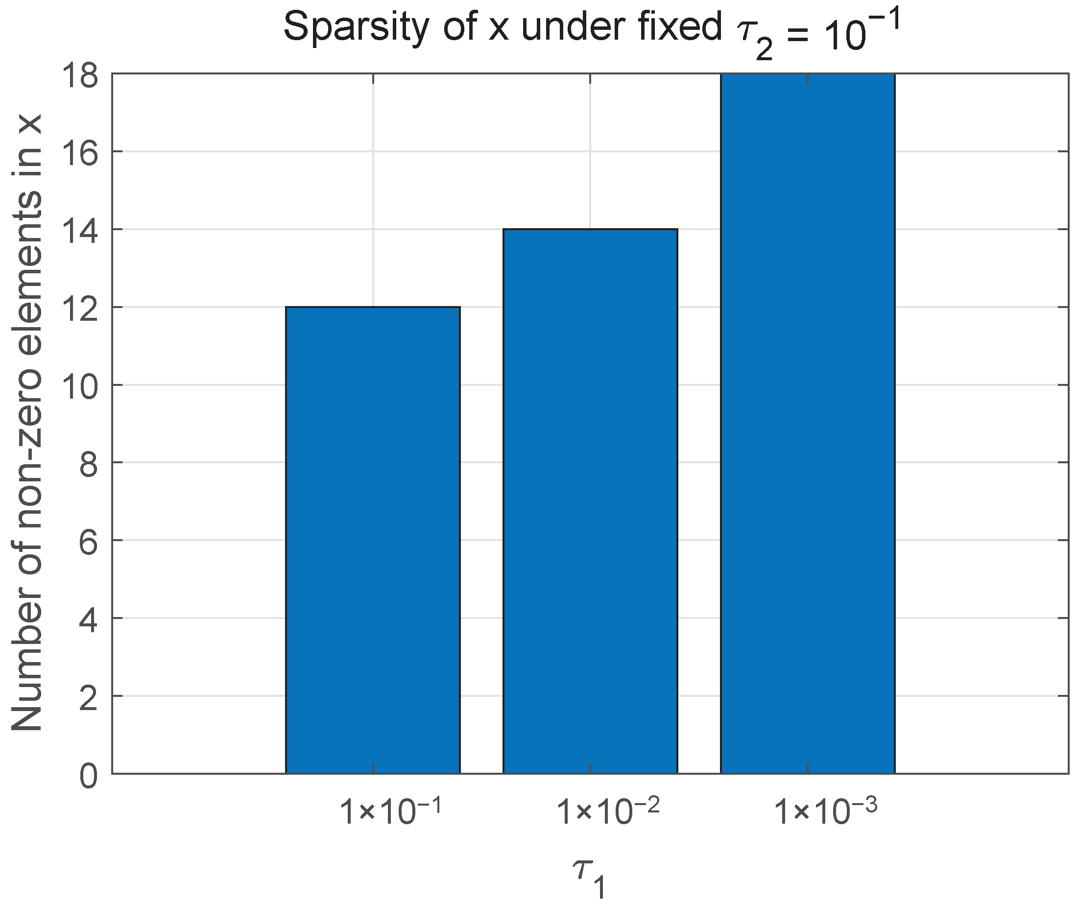
A closer examination of Table 1 reveals that the effects of τ 1 and τ 2 are not symmetric. When τ 1 is held fixed, increasing τ 2 causes more drastic changes in the objective function, suggesting that the CVaR-related regularization term ( τ 2 ) has a more sensitive and dominant influence on the optimization outcome in this context. To further analyze the effect of τ 1 , Figure 2 presents the objective trends as τ 1 varies while τ 2 is fixed.
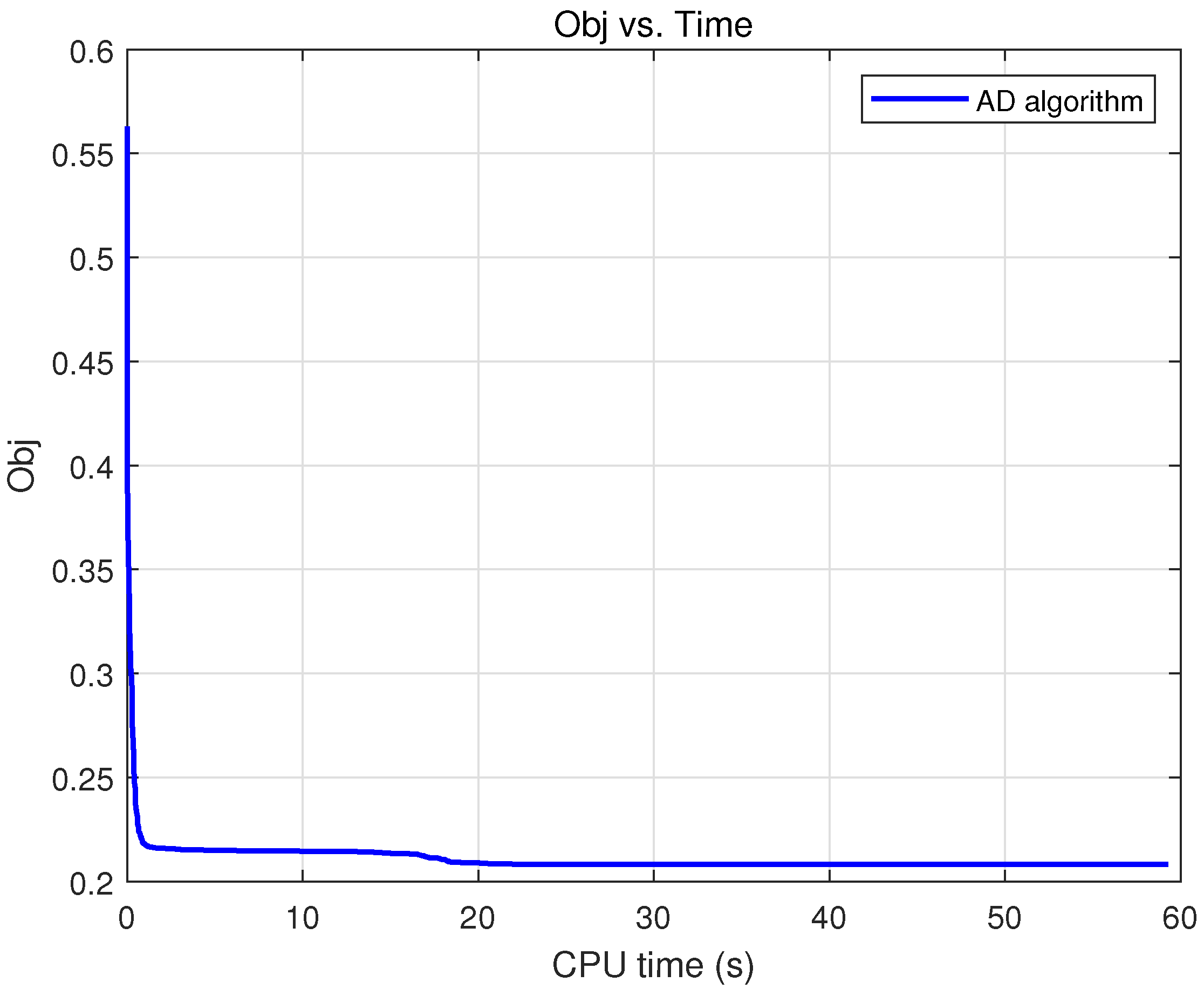
Moreover, Figure 3 depicts the convergence trajectory of Obj with respect to CPU time under the settings τ 1 = 10 3 and τ 2 = 10 3 . The curve indicates that the AD algorithm converges rapidly, with Obj reaching a relatively stable value within approximately 1.6 s. The algorithm continues running up to 60 s only due to the preset stopping criterion of 1000 iterations. Similar convergence behavior is observed under other parameter configurations, further confirming the stability and computational efficiency of our AD algorithm.

6. Conclusions

In this paper, we propose a sparse model that combines DRO and the CVaR penalty, where the CVaR penalty can be replaced by other convex functions. We transform the model to an equivalent non-smooth positive semi-definite type of programming, where the non-smoothness arises from the maximum of numerous non-smooth functions. An approximate discretization algorithm of the non-smooth positive semi-definite programming is provided, which is convergent under mild conditions. This discretization scheme of the equivalent reformulation can be solved directly by a subgradient method or a smoothing projected-gradient method. We propose an approximate discretization (AD) algorithm by combining a low-complexity subgradient method with the preceding transformation. Furthermore, numerical experiments on a portfolio optimization problem validate the effectiveness and efficiency of the AD algorithm in real-world scenarios.

Author Contributions

Conceptualization, R.W., Q.G., C.L. and Y.H.; methodology, R.W., Q.G., C.L. and Y.H.; writing—original draft preparation, R.W., Q.G. and C.L.; writing—review and editing, Q.G. and Y.H.; supervision, Q.G. and Y.H.; funding acquisition, R.W., Q.G. and Y.H. All authors have read and agreed to the published version of the manuscript.

Funding

This research was supported by the Scientific Startup Foundation for Doctors of Northwest A& F University (Z1090324139, Z1090125002), the Natural Sciences and Engineering Research Council of Canada (RGPIN 2024-05941), and a centennial fund from the University of Alberta.

Institutional Review Board Statement

Not applicable.

Informed Consent Statement

Not applicable.

Data Availability Statement

No new data were created or analyzed in this study. Data sharing is not applicable to this article.

Conflicts of Interest

The authors declare no conflicts of interest.

References

  1. Beyer, H.G.; Sendhoff, B. Robust optimization—A comprehensive survey. Comput. Methods Appl. Mech. Eng. 2007, 196, 3190–3218. [Google Scholar] [CrossRef]
  2. Bertsimas, D.; Brown, D.B.; Caramanis, C. Theory and applications of robust optimization. SIAM Rev. 2011, 53, 464–501. [Google Scholar] [CrossRef]
  3. Gabrel, V.; Murat, C.; Thiele, A. Recent advances in robust optimization: An overview. Eur. J. Oper. Res 2014, 235, 471–483. [Google Scholar] [CrossRef]
  4. Delage, E.; Ye, Y. Distributionally robust optimization under moment uncertainty with application to data-driven problems. Oper. Res. 2010, 58, 595–612. [Google Scholar] [CrossRef]
  5. Rahimian, H.; Mehrotra, S. Distributionally robust optimization: A review. arXiv 2019. [Google Scholar] [CrossRef]
  6. Levy, D.; Carmon, Y.; Duchi, J.C.; Sidford, A. Large-scale methods for distributionally robust optimization. Adv. Neural Inf. Process. Syst. 2020, 33, 8847–8860. [Google Scholar]
  7. Shapiro, A.; Zhou, E.; Lin, Y. Bayesian distributionally robust optimization. SIAM J. Optim. 2023, 33, 1279–1304. [Google Scholar] [CrossRef]
  8. Fan, Z.; Ji, R.; Lejeune, M.A. Distributionally robust portfolio optimization under marginal and copula ambiguity. J. Optim. Theory Appl. 2024, 203, 2870–2907. [Google Scholar] [CrossRef]
  9. Rockafellar, R.T.; Uryasev, S. Optimization of Conditional Value-at-Risk. J. Risk. Res. 2000, 2, 21–42. [Google Scholar] [CrossRef]
  10. Noyan, N. Risk-averse two-stage stochastic programming with an application to disaster management. Comput. Oper. Res. 2012, 39, 541–559. [Google Scholar] [CrossRef]
  11. Arpón, S.; Homem-de Mello, T.; Pagnoncelli, B. Scenario reduction for stochastic programs with Conditional Value-at-Risk. Math. Program. 2018, 170, 327–356. [Google Scholar] [CrossRef]
  12. Anderson, E.; Xu, H.; Zhang, D. Varying confidence levels for CVaR risk measures and minimax limits. Math. Program. 2020, 180, 327–370. [Google Scholar] [CrossRef]
  13. Behera, J.; Pasayat, A.K.; Behera, H.; Kumar, P. Prediction based mean-value-at-risk portfolio optimization using machine learning regression algorithms for multi-national stock markets. Eng. Appl. Artif. Intell. 2023, 120, 105843. [Google Scholar] [CrossRef]
  14. Yang, C.; Wu, Z.; Li, X.; Fars, A. Risk-constrained stochastic scheduling for energy hub: Integrating renewables, demand response, and electric vehicles. Energy 2024, 288, 129680. [Google Scholar] [CrossRef]
  15. Brodie, J.; Daubechies, I.; De Mol, C.; Giannone, D.; Loris, I. Sparse and stable Markowitz portfolios. Proc. Natl. Acad. Sci. USA 2009, 106, 12267–12272. [Google Scholar] [CrossRef] [PubMed]
  16. Fastrich, B.; Paterlini, S.; Winker, P. Constructing optimal sparse portfolios using regularization methods. Comput. Manag. Sci. 2015, 12, 417–434. [Google Scholar] [CrossRef]
  17. Dai, Z.; Wen, F. Some improved sparse and stable portfolio optimization problems. Financ. Res. Lett. 2018, 27, 46–52. [Google Scholar] [CrossRef]
  18. Chai, B.; Eisenbart, B.; Nikzad, M.; Fox, B.; Blythe, A.; Blanchard, P.; Dahl, J. Simulation-based optimisation for injection configuration design of liquid composite moulding processes: A review. Compos. Part A Appl. Sci. Manuf. 2021, 149, 106540. [Google Scholar] [CrossRef]
  19. Wijaya, W.; Bickerton, S.; Kelly, P. Meso-scale compaction simulation of multi-layer 2D textile reinforcements: A Kirchhoff-based large-strain non-linear elastic constitutive tow model. Compos. Part A Appl. Sci. Manuf. 2020, 137, 106017. [Google Scholar] [CrossRef]
  20. Ali, M.A.; Irfan, M.S.; Khan, T.; Khalid, M.Y.; Umer, R. Graphene nanoparticles as data generating digital materials in industry 4.0. Sci. Rep. 2023, 13, 4945. [Google Scholar] [CrossRef]
  21. Xu, H.; Liu, Y.; Sun, H. Distributionally robust optimization with matrix moment constraints: Lagrange duality and cutting plane methods. Math. Program. 2018, 169, 489–529. [Google Scholar] [CrossRef]
  22. Boyd, S.P.; Vandenberghe, L. Convex Optimization; Cambridge University Press: Cambridge, UK, 2004. [Google Scholar]
  23. Sion, M. On general minimax theorems. Pac. J. Math. 1958, 8, 171–176. [Google Scholar] [CrossRef]
  24. Shapiro, A. On duality theory of conic linear problems. In Semi-Infinite Programming; Springer: New York, NY, USA, 2001; pp. 135–165. [Google Scholar]
  25. Mordukhovich, B.; Nam, N.M. An Easy Path to Convex Analysis and Applications; Springer Nature: Berlin/Heidelberg, Germany, 2014. [Google Scholar]
  26. Shapiro, A.; Xu, H. Stochastic mathematical programs with equilibrium constraints, modelling and sample average approximation. Optimization 2008, 57, 395–418. [Google Scholar] [CrossRef]
  27. Polyak, B.T. Subgradient methods: A survey of Soviet research. In Proceedings of the Nonsmooth Optimization: Proceedings of a IIASA Workshop, Laxenburg, Austria, 28 March–8 April 1977; pp. 5–29. [Google Scholar]
  28. Boyd, S.; Xiao, L.; Mutapcic, A. Subgradient Methods; Lecture Notes of EE392o; Stanford University: Stanford, CA, USA, 2004. [Google Scholar]
  29. Nedic, A.; Bertsekas, D.P. Incremental subgradient methods for nondifferentiable optimization. SIAM J. Optim. 2001, 12, 109–138. [Google Scholar] [CrossRef]
  30. Chen, X. Smoothing methods for nonsmooth, nonconvex minimization. Math. Program. 2012, 134, 71–99. [Google Scholar] [CrossRef]
  31. Zhang, C.; Chen, X. Smoothing projected gradient method and its application to stochastic linear complementarity problems. SIAM J. Optim. 2009, 20, 627–649. [Google Scholar] [CrossRef]
  32. Zhang, C.; Chen, X. A smoothing active set method for linearly constrained non-lipschitz nonconvex optimization. SIAM J. Optim. 2020, 30, 1–30. [Google Scholar] [CrossRef]
  33. Sant’Anna, L.R.; Caldeira, J.F.; Filomena, T.P. Lasso-based index tracking and statistical arbitrage long-short strategies. N. Amer. J. Econ. Financ. 2020, 51, 101055. [Google Scholar] [CrossRef]
  34. Wiesemann, W.; Kuhn, D.; Sim, M. Distributionally robust convex optimization. Oper. Res. 2014, 62, 1358–1376. [Google Scholar] [CrossRef]
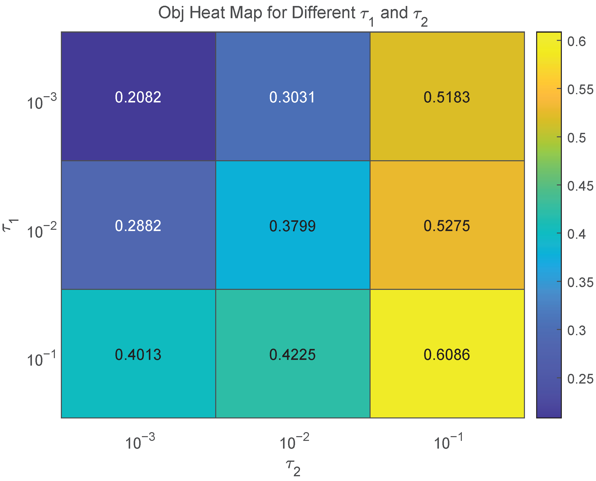
Figure 1. The objective value heat map for different τ 1 and τ 2 .
Information 16 00676 g001
Figure 2. Sparsity of solution vector x under different parameter settings.
Information 16 00676 g002
Figure 3. Obj vs. CPU time under τ 1 = 10 3 and τ 2 = 10 3 .
Information 16 00676 g003
Table 1. Obj and CPU time under different parameter settings.
τ 1 τ 2 ObjCPU Time
10 3 10 3 0.208259.9984
10 3 10 2 0.303174.0531
10 3 10 1 0.518378.4453
10 2 10 3 0.288268.1875
10 2 10 2 0.379976.6968
10 2 10 1 0.527579.2125
10 1 10 3 0.401369.6593
10 1 10 2 0.422577.2062
10 1 10 1 0.608680.0687
Disclaimer/Publisher’s Note: The statements, opinions and data contained in all publications are solely those of the individual author(s) and contributor(s) and not of MDPI and/or the editor(s). MDPI and/or the editor(s) disclaim responsibility for any injury to people or property resulting from any ideas, methods, instructions or products referred to in the content.