Incremental Beta Distribution Weighted Fuzzy C-Ordered Means Clustering

Abstract

Streaming data is becoming more and more common in the field of big data and incremental frameworks can address its complexity. The BDFCOM algorithm achieves good results on common form datasets by introducing the ordering mechanism of beta distribution weighting. In this paper, based on the BDFCOM algorithm, two incremental beta distribution weighted fuzzy C-ordered means clustering algorithms, SPBDFCOM and OBDFCOM, are proposed by combining the two incremental frameworks of Single-Pass and Online, respectively. In order to validate the performance of SPBDFCOM and OBDFCOM, this paper selects seven real datasets for experiments and compares their performance with six other incremental clustering algorithms using six evaluation metrics. The results show that the two proposed incremental algorithms perform significantly better compared to other algorithms.

1. Introduction

In the era of big data, the quality of data processing capabilities is particularly important. With an increase in data volume, how to effectively extract valuable information from it has become an urgent problem. Among many data analysis methods, fuzzy clustering, as an excellent technical tool, has received widespread attention for its ability to deal with uncertainty and ambiguity in data. Fuzzy clustering can not only divide the sample points into different clusters, but also assign a degree of membership to each sample point, reflecting its degree of membership to each cluster [1,2,3]. This characteristic makes fuzzy clustering a strong advantage in many practical application scenarios, especially in the fields of image segmentation, text classification and social network research [4,5,6].

With the continuous development of fuzzy clustering algorithms, researchers have gradually found that they have certain limitations in dealing with certain complex data sets. To solve this problem, ordered mechanisms are introduced, i.e., ordered weights are introduced in the clustering process to guide the sample points to different clusters. FCOM (Fuzzy C-Ordered Means), as the first of these proposed mechanisms, greatly enriches the theoretical system of fuzzy clustering [7]. On this basis, Wang further proposed BDFCOM (Beta Distributed Fuzzy C-Ordered Means) as an improved version of FCOM, which not only inherits the advantages of the ordered mechanism, but also improves the cumbersome sorting process by introducing beta distribution as an attribute weighting strategy, making the clustering more flexible and precise [8].

Big data is not just static, it is real-time and continuous. The emergence of streaming data has led to new challenges in data analysis [9,10]. This type of data is generated at high speed and continuously, such as sensor data, network data and financial data [11,12,13]. To address the complexity of streaming data, incremental frameworks have been gradually introduced into clustering algorithms. Incremental frameworks allow algorithms to update clustering results in real time without reprocessing all the historical data, which greatly improves the efficiency of data processing [14,15]. Currently, Single-Pass and Online are two commonly used incremental frameworks that have been successfully applied to FCOM clustering algorithms. Although these two incremental frameworks address the inability of FCOM to handle streaming data, various evaluation metrics still need to be improved [16,17].

In order to further improve the performance of fuzzy clustering with ordered mechanism in dealing with streaming data, this paper proposes two incremental beta distribution weighted fuzzy c-ordered means clustering algorithms—SPBDFCOM and OBDFCOM. These two algorithms improve on BDFCOM by combining the Single-Pass and Online incremental frameworks, so that they not only inherit the ability of beta distributed c-ordered weighting to deal with static data, which allows the algorithms to be dynamically adjusted according to the importance of the data points during the clustering process, but also have relatively high performance when dealing with the challenges of streaming data.

In this paper, seven real datasets are selected for experiments and the performance of the two proposed algorithms is compared with six other incremental clustering algorithms with six evaluation metrics. The results show that the two proposed incremental algorithms are able to maintain high clustering quality compared to other algorithms.

2. Related Work

2.1. Beta Distribution Weighted Fuzzy C-Ordered-Means Clustering (BDFCOM)

In order to optimize the weights of feature attributes, the BDFCOM algorithm introduces beta distribution on the basis of FCOM to calculate the feature weights. This makes the algorithm more flexible and enables it to dynamically reflect the influence of different attributes on the clustering results [8].

In comparison to alternative weighting methodologies, beta distribution enables the regulation of weight distribution patterns through the manipulation of two shape parameters (α and β), thereby enhancing the algorithm’s adaptability in addressing the discrepancies inherent in data features. This design facilitates the accentuation of the impact of pivotal features on the outcomes, ultimately leading to superior clustering results.

2.2. Incremental Frameworks (Single-Pass and Online)

When the amount of data to be clustered becomes increasingly large and a combination of previous and new data has to be considered, the best approach is to incrementally update the new clustering results based on the old data, rather than re-scanning from scratch and re-analyzing all the data [18].

In order to deal with the problem of massive data, Hore proposed the SPFCM and the OFCM [19,20].

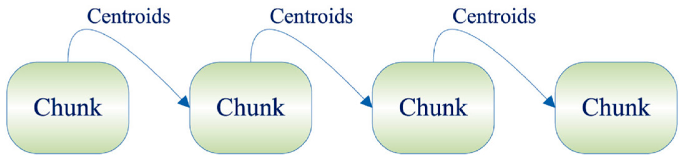
Among them, the basic idea of the Single-Pass incremental framework is to divide all sample datasets into several data chunks. Firstly, the first data chunk is clustered, and after obtaining the cluster centroids and corresponding weights, it is involved in the next data chunk until the last data chunk is computed [19]. The specific process is shown in Figure 1.

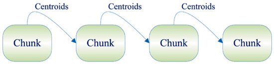
Figure 1. Single-Pass framework.

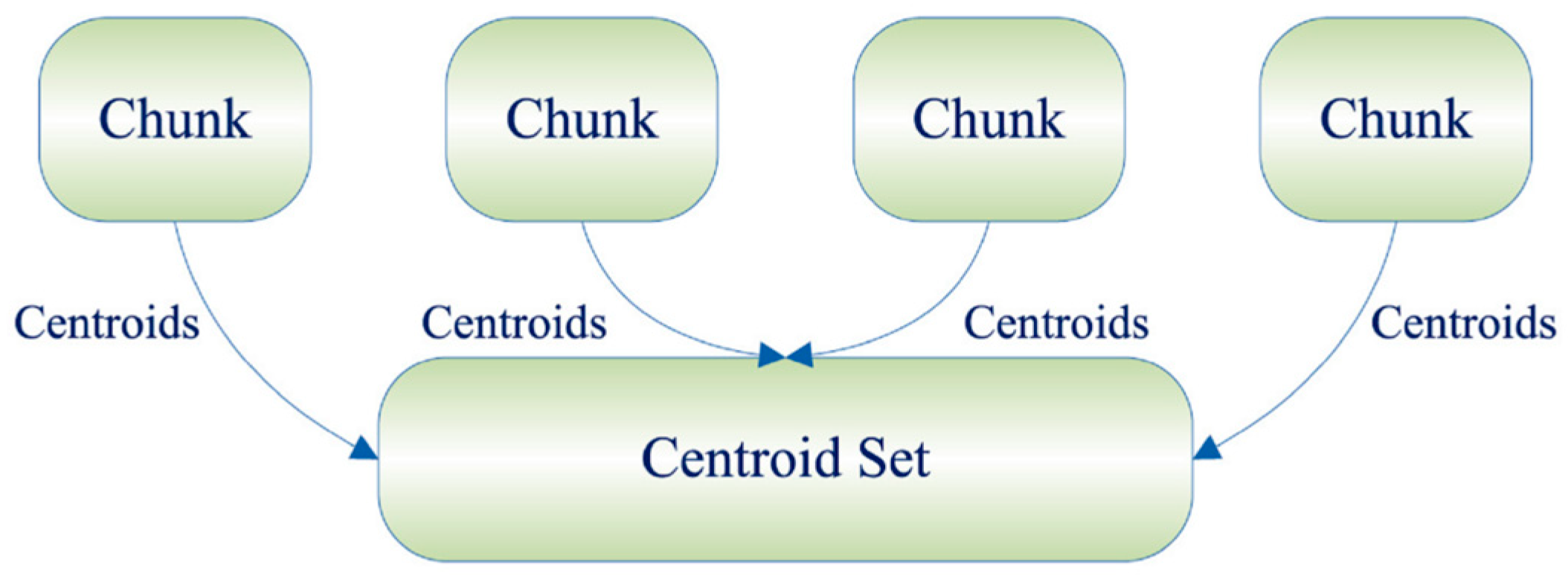
In contrast, the Online incremental framework divides the entire sample data set into several data chunks, clusters all the data chunks individually, and after obtaining the cluster centroids and the corresponding weight matrices, inserts them into the empty data chunk matrices and weight matrices for the final clustering operation [20]. The specific process is shown in Figure 2.

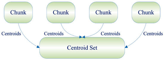
Figure 2. Online framework.

3. Incremental Beta Distribution Fuzzy C-Ordered Means Clustering

Firstly, the BDFCOM algorithm is weighted in order to adopt the Single-Pass and Online incremental frameworks.

The objective function of WBDFCOM is defined as follows:

$$J(U,V)=\sum _{c=1}^C\sum _{i=1}^N{{\rho }_i\omega }_{ci}\left(u_{ci}{)}^{m}D\right(x_i,v_c)$$

(1)

where U is the C × N membership matrix and each element u_ci (u_ci ∈ [0, 1]) represents the membership of each sample to each cluster; the parameter ω_ci denotes the weighted value of the beta distribution of the ith data to the cth cluster; ${\rho }_i$ is the weight corresponding to the ith data, which is later applied in the Single-Pass and Online incremental frameworks. D(x_i, v_c) is computed by H_cij and E_cij as follows:

$$D(x_i,v_c)=\sum _{j=1}^{K}D\left(x_{ij},v_{cj}\right)=\sum _{j=1}^K{H}_{cij}{E}_{cij}^2$$

(2)

where E_cij is the distance between x_ij and v_cj (the distance between the jth attribute of the ith sample and the jth attribute of the center of mass of the cth cluster), as follows:

$$E_{cij}=x_{ij}-v_{cj}$$

(3)

H_cij is a weighted robust parameter [21]. The main methods are as follows:

$$H_{cij}=\left\{\begin{array}{cc}0,\hfill & E_{cij}=0\hfill \\ \mathcal{L}\left(E_{cij}\right)/(E_{cij}{)}^2,\hfill & E_{cij}\ne 0\hfill \end{array}\right.$$

(4)

$$H_{cij}=\left\{\begin{array}{cc}0,\hfill & E_{cij}=0\hfill \\ 1/\left|E_{cij}\right|,\hfill & E_{cij}\ne 0\hfill \end{array}\right.$$

(5)

$$H_{cij}=\left\{\begin{array}{cc}1/{\delta }^2,\hfill & \left|E_{cij}\right|\le \delta \hfill \\ 1/\left(\delta \right|E_{cij}\left|\right),\hfill & \left|E_{cij}\right|>\delta \hfill \end{array}\right.$$

(6)

$$H_{cij}=\left\{\begin{array}{cc}0,\hfill & E_{cij}=0\hfill \\ {\displaystyle \frac{1}{\left\{\right(E_{cij}{)}^2[1+\mathit{exp}(-\alpha (\left|E_{cij}\right|-\beta \left)\right)\left]\right\}}},\hfill & E_{cij}\ne 0\hfill \end{array}\right.$$

(7)

$$H_{cij}=\left\{\begin{array}{cc}0,\hfill & E_{cij}=0\hfill \\ {\displaystyle \frac{1}{\left\{E_{cij}\right[1+\mathit{exp}(-\alpha \left(\right|E_{cij}|-\beta )\left)\right]\}}},\hfill & E_{cij}\ne 0\hfill \end{array}\right.$$

(8)

$$H_{cij}=\left\{\begin{array}{cc}0,\hfill & E_{cij}=0\hfill \\ \mathit{log}(1+E_{cij}^2)/E_{cij}^2,\hfill & E_{cij}\ne 0\hfill \end{array}\right.$$

(9)

$$H_{cij}=\left\{\begin{array}{cc}0,\hfill & E_{cij}=0\hfill \\ \mathit{log}(1+E_{cij}^2)/|E_{cij}|,\hfill & E_{cij}\ne 0\hfill \end{array}\right.$$

(10)

The constraints on the objective function of WBDFCOM are as follows:

$$\left\{\begin{array}{c}\underset{\begin{array}{c}1\le c\le C\\ 1\le i\le N\end{array}}{\forall }{u}_{ci}\in \left[\mathrm{0,1}\right];\\ {\displaystyle \sum _{c=1}^C}{\omega }_{ci}{u}_{ci}=T_i;\\ 0<{\displaystyle \sum _{i=1}^N}{u}_{ci}<N.\end{array}\right.$$

(11)

where, T_i is the global beta distribution weighted value about the ith sample, i.e., the combined typicality assessment of the ith sample about all attributes for all clusters. Calculate T_i through the maximum value method in S-norm, as follows:

$$\underset{1\le i\le N}{\forall }{T}_i={\omega }_{1i}\vee {\omega }_{2i}\vee {\omega }_{3i}\vee \dots \vee {\omega }_{ci}$$

(12)

For the beta distribution weighted value ω_ci of the ith sample for the cth cluster, it is calculated by the algebraic product method in T-norm as follows:

$$\underset{\begin{array}{c}1\le c\le C\\ 1\le i\le N\end{array}}{\forall }{\omega }_{ci}={\omega }_{ci1}\cdot {\omega }_{ci2}\cdot {\omega }_{ci3}\cdot \dots \cdot {\omega }_{cij}$$

(13)

where the parameter ω_cij denotes the beta distribution weighted value of the jth attribute of the ith sample to the jth attribute of the cth cluster. After determining the order using Equation (14), bring Y_i to x in Equations (15) and (16) to obtain ω_cij. In this case, we also use PCHI (Piecewise Cubic Hermitian Interpolation) to improve the efficiency of the operation. After obtaining ω_cij, ω_ci is computed as follows:

$$Y_i={\displaystyle \frac{E_{cij}-\underset{1\le i\le N}{min}\left\{E_{cij}\right\}}{\underset{1\le i\le N}{max}\left\{E_{cij}\right\}-\underset{1\le i\le N}{min}\left\{E_{cij}\right\}}}$$

(14)

$$f\left(x; \alpha ,\beta \right)={\displaystyle \frac{x^{\alpha -1}\ast {(1-x)}^{\beta -1}}{B(\alpha ,\beta )}}$$

(15)

$$B\left(\alpha ,\beta \right)={\int }_0^1{t}^{\alpha -1}\ast {(1-t)}^{\beta -1}dt$$

(16)

According to the constraint Equation (11), applying the Lagrange multiplier method to Equation (1), a new objective function is constructed to make it obtain the minimum value, as follows:

$$J\left(U,V;{\lambda }_i\right)=\sum _{c=1}^C\sum _{i=1}^N{{\rho }_i\omega }_{ci}\left(u_{ci}{)}^{m}D\right(x_i,v_c)-{\lambda }_i\left[\sum _{c=1}^C{\omega }_{ci}{u}_{ci}-T_i\right]$$

(17)

Using Equation (17) for U to obtain a partial derivation and setting to zero yields, as follows:

$${\displaystyle \frac{\partial J}{\partial U}}=m{\rho }_i{\omega }_{ci}(u_{ci}{)}^{m-1}D(x_i,v_c)-{\lambda }_k{\omega }_{ci}=0$$

(18)

The u_ci can be obtained from Equations (11) and (18), as follows:

$$\underset{\begin{array}{c}1<i<N\\ 1<c<C\end{array}}{\forall }{u}_{ci}={\displaystyle \frac{T_{i}D(x_i,v_c{)}^{\frac{1}{1-m}}}{\left[{\sum }_{t=1}^C{\omega }_{ti}D(x_i,v_t{)}^{\frac{1}{1-m}}\right]}}$$

(19)

Similarly, using Equation (17) to partialize and set zero for V yields, as follows:

$${\displaystyle \frac{\partial J}{\partial V}}=-2\sum _{i=1}^N{{\rho }_i\omega }_{ci}\left(u_{ci}{)}^m{H}_{cij}\right(x_{ij}-v_{cj})=0$$

(20)

The v_cj can be obtained from Equations (11) and (20), as follows:

$$\underset{\begin{array}{c}1<c<C\\ 1<j<K\end{array}}{\forall }{v}_{cj}={\displaystyle \frac{\left[{\sum }_{i=1}^N{{\rho }_i\omega }_{ci}(u_{ci}{)}^m{H}_{cij}{x}_{ij}\right]}{\left[{\sum }_{i=1}^N{{\rho }_i\omega }_{ci}(u_{ci}{)}^m{H}_{cij}\right]}}$$

(21)

And then, we will design two Incremental Beta Distribution Fuzzy C-Ordered Means Clustering by Single-Pass and Online frameworks.

3.1. Single-Pass Beta Distribution Fuzzy C-Ordered Means Clustering (SPBDFCOM)

Firstly, the dataset is divided into R chunks, i.e., X¹ to X^R, according to some requirements. Secondly, the weights of all the samples for the clusters are initialized to 1, i.e., as follows:

$${InitialWeight}^{chunk} = {[{iw}^1,{iw}^2,\dots ,{iw}^R]}^T$$

(22)

where the number of elements in each iw is the number of samples in the corresponding data chunk and the elements all take the value of 1.

(1) When the data chunk number r = 1, according to Equations (19) and (21), the iterative formulas for u_ci and v_cj in data chunk X¹ can be obtained as follows:

$$u_{ci}={\displaystyle \frac{T_{i}D(x_i,v_c{)}^{\frac{1}{1-m}}}{\left[{\sum }_{t=1}^C{\omega }_{ti}D(x_i,v_t{)}^{\frac{1}{1-m}}\right]}}$$

(23)

$$v_{cj}={\displaystyle \frac{\left[{\sum }_{i=1}^N{{\rho }_i\omega }_{ci}(u_{ci}{)}^m{H}_{cij}{x}_{ij}\right]}{\left[{\sum }_{i=1}^N{{\rho }_i\omega }_{ci}(u_{ci}{)}^m{H}_{cij}\right]}}$$

(24)

where $1\le j\le K,1\le i\le n_1,1\le c\le C,{\rho }_i={iw}_i^1$.

After clustering the first data chunk X¹, the cluster centroid ${\Delta }^1=[v_1,v_2,\dots ,v_c]$ and the corresponding weight weight¹ are obtained as follows:

$${weight}_c^1=\sum _{l=1}^{n_1}\left(u_{cl}\right){iw}_l^1$$

(25)

where $1\le c\le C, \forall 1\le l\le n_1.$ n₁ is the number of samples in the first data chunk.

(2) When r > 1, the cluster centroids obtained last time are added to the r-th data chunk and the weight matrix obtained last time is also added to the corresponding sample weights to obtain a new data chunk ${{\mathit{X}}^r}^{\prime }$ and its weight matrix $\rho$ as follows:

$${X^r}^{\prime }=\left[{\Delta }^1, X^r\right]$$

(26)

$$\rho =\left[{weight}_1^{r-1}, {\dots ,{weight}_C^{r-1},iw}^r\right]$$

(27)

Based on Equations (19) and (21), the iterative formulas for u_ci and v_cj in the r-th data chunk can be obtained as follows:

$$u_{ci}={\displaystyle \frac{T_{i}D(x_i,v_c{)}^{\frac{1}{1-m}}}{\left[{\sum }_{t=1}^C{\omega }_{ti}D(x_i,v_t{)}^{\frac{1}{1-m}}\right]}}$$

(28)

$$v_{cj}={\displaystyle \frac{\left[{\sum }_{i=1}^N{{\rho }_i\omega }_{ci}(u_{ci}{)}^m{H}_{cij}{x}_{ij}\right]}{\left[{\sum }_{i=1}^N{{\rho }_i\omega }_{ci}(u_{ci}{)}^m{H}_{cij}\right]}}$$

(29)

where $1\le j\le K,1\le i\le n_r+c,1\le c\le C$.

The SPBDFCOM algorithm can be expressed in pseudo-code as follows:

Step 1. Determine the number of clusters C and the weight index m∈(1, ∞). Choose the ε—sensitivity dissimilarity measure. Choose the weighted robustness parameter computation method. Select the values of α and β for controlling the slope. Initialize the membership matrix U⁽⁰⁾. Set the iteration threshold ξ. ω_ci = 1, H_cij = 1, T_i = 1 and number of iterations T = 1.

Step 2. Divide the dataset into R data chunks, i.e., X¹ to X^R, initialize the weight matrix ${InitialWeight}^{chunk} = {[{iw}^1,{iw}^2,\dots ,{iw}^R]}^T$, initialize the data chunks serial number r = 1;

Step 3. Update the cluster center matrix V^(T) using Equations (24) or (29);

Step 4. Update the residual E_cij using Equation (3);

Step 5. Update the weighted robustness parameter H_cij using Equations (4)–(10);

Step 6. Calculate the dissimilarity metric distance D_ci using Equation (2);

Step 7. Calculate the ordered ordinal number Y_i using Equation (14);

Step 8. Calculate the beta distribution weight of each attribute per sample for each attribute per cluster ω_cij using interpolation function PCHI;

Step 9. Calculate the beta distribution weight of each attribute per sample for each cluster ω_ci using Equation (13);

Step 10. Calculate the beta distribution weight for each sample T_i using Equation (12);

Step 11. Update the membership matrix U^(T) using Equations (23) or (28);

Step 12. ① If r < R: If ||U^(T) − U^(T−1)||_F > ξ, set T ← T + 1 and go to Step 3; otherwise add the cluster centroids and weight matrices to the next data chunk, set r ← r + 1 and go to Step 3;

② If r = R: If ||U^(T) − U^(T−1)||_F > ξ, make T ← T + 1 and go to Step 3; otherwise end.

3.2. Online Beta Distribution Weighted Fuzzy C-Ordered-Means (OBDFCOM)

Firstly, the dataset is divided into R chunks, i.e., X¹ to X^R, according to some requirements. Secondly, the weights of all the samples for the clusters are initialized to 1, i.e., ${InitialWeight}^{chunk} = {[{iw}^1,{iw}^2,\dots ,{iw}^R]}^T$, where the number of elements in each iw is the number of samples in the corresponding data chunk and the elements all take the value of 1.

(1) Clustering each data chunk separately and individually, according to Equations (19) and (21), the iterative formulas for the sample membership u_ci and the cluster centroid v_cj for the r-th data chunk can be obtained as follows:

$$u_{ci}={\displaystyle \frac{T_{i}D(x_i,v_c{)}^{\frac{1}{1-m}}}{\left[{\sum }_{t=1}^C{\omega }_{ti}D(x_i,v_t{)}^{\frac{1}{1-m}}\right]}}$$

(30)

$$v_{cj}={\displaystyle \frac{\left[{\sum }_{i=1}^N{{\rho }_i\omega }_{ci}(u_{ci}{)}^m{H}_{cij}{x}_{ij}\right]}{\left[{\sum }_{i=1}^N{{\rho }_i\omega }_{ci}(u_{ci}{)}^m{H}_{cij}\right]}}$$

(31)

where $1\le j\le K,1\le i\le n_r,1\le c\le C,{\rho }_i=1.$

After clustering each data chunk X^r, the cluster centroids ${\Delta }^r=[v_1^r,v_2^r,\dots ,v_c^r]$ and the corresponding weight matrices ${weight}^r=[{weight}_1^r,{weight}_2^r,\dots ,{weight}_c^r]$ are obtained for each data chunk.

(2) After clustering each data chunk, obtain the cluster centroid matrix and the corresponding weight matrix, which are aggregated to form a new cluster centroid matrix and weight matrix, as follows:

$$X^{\prime }=\left[\begin{array}{c}{\Delta }_1^1,\dots ,{\Delta }_c^1,\\ {\Delta }_1^2,\dots ,{\Delta }_c^2,\\ \dots ,\\ {\Delta }_1^r,\dots ,{\Delta }_c^r\end{array}\right]$$

(32)

$$\rho =\left[\begin{array}{c}{weight}_1^1,{\dots ,weight}_c^1,\\ {weight}_1^2 ,\dots ,{weight}_c^2,\\ \dots ,\\ {weight}_1^r,\dots ,{weight}_c^r\end{array}\right]$$

(33)

Then, cluster the new cluster centroid matrix $X^{\prime }$. According to Equations (19) and (21), the iterative formulae for the sample membership u_ci and the cluster centroids v_cj in the data chunk $X^{\prime }$ can be obtained as follows:

$$u_{ci}={\displaystyle \frac{T_{i}D(x_i,v_c{)}^{\frac{1}{1-m}}}{\left[{\sum }_{t=1}^C{\omega }_{ti}D(x_i,v_t{)}^{\frac{1}{1-m}}\right]}}$$

(34)

$$v_{cj}={\displaystyle \frac{\left[{\sum }_{i=1}^N{{\rho }_i\omega }_{ci}(u_{ci}{)}^m{H}_{cij}{x}_{ij}\right]}{\left[{\sum }_{i=1}^N{{\rho }_i\omega }_{ci}(u_{ci}{)}^m{H}_{cij}\right]}}$$

(35)

where $1\le j\le K,1\le i\le C\ast R,1\le c\le C.$

The OBDFCOM algorithm can be expressed in pseudo-code as follows:

Step 1. Determine the number of clusters C and the weight index m∈(1, ∞). Choose the ε- sensitivity dissimilarity measure. Choose the weighted robustness parameter computation method. Select the values of α and β for controlling the slope. Initialize the membership matrix U⁽⁰⁾. Initialize the cluster centroid matrix $X^{\prime }$ and the weight matrix $\rho$. Set the iteration threshold ξ. ω_ci = 1, H_cij = 1, T_i = 1 and number of iterations T = 1;

Step 2. Divide the dataset into R data chunks, i.e., X¹ to X^R, initialize the weight matrix ${InitialWeight}^{chunk} = {[{iw}^1,{iw}^2,\dots ,{iw}^R]}^T$, initialize the data chunks serial number r = 1;

Step 3. Update the cluster center matrix V^(T) using Equations (31) or (35);

Step 4. Update the residual E_cij using Equation (3);

Step 5. Update the weighted robustness parameter H_cij using Equations (4)–(10);

Step 6. Calculate the dissimilarity metric distance D_ci using Equation (2);

Step 7. Calculate the ordered ordinal number Y_i using Equation (14);

Step 8. Calculate the beta distribution weight of each attribute per sample for each attribute per cluster ω_cij using interpolation function PCHI;

Step 9. Calculate the beta distribution weight of each attribute per sample for each cluster ω_ci using Equation (13);

Step 10. Calculate the Beta distribution weight for each sample T_i using Equation (12);

Step 11. Update the membership matrix U^(T) using Equations (30) or (34);

Step 12. ① If r < R: If ||U^(T) − U^(T−1)||_F > ξ, set T ← T + 1 and go to Step 3. Otherwise, add the cluster centroids and weight matrices to the cluster centroid matrix $X^{\prime }$ and the weight matrix $\rho$, respectively, set r ← r + 1 and go to Step 3;

② If r = R: If ||U^(T) − U^(T−1)||_F > ξ, set T ← T + 1 and go to Step 3. Otherwise, add the cluster centroids and weight matrices to the cluster centroid matrix $X^{\prime }$ and the weight matrix $\rho$, respectively, set r = $X^{\prime }$ and go to Step 3;

③ If r = $X^{\prime }$: If ||U^(T) − U^(T−1)||_F > ξ, make T ← T + 1 and go to Step 3, otherwise end.

4. Analysis and Results

4.1. Experimental Datasets

To evaluate the performance of the SPBDFCOM and OBDFCOM algorithms, seven datasets were selected from the UCI database and Kaggle for the experiments. The information for each dataset is shown in Table 1. The experimental data used for the experiments in this paper are real datasets [22,23,24,25].

Table 1. Experimental datasets.

Dataset	Sample Size	Attribute Count	Cluster Number	Source	Domain
Breast Tissue (BT)	106	9	6	UCI	Medical dataset
Zoo	101	16	7	UCI	Animal dataset
Mice	1077	68	8	UCI	Medical dataset
HCV	589	12	2	UCI	Medical dataset
Shill Bidding Data (SBD)	6321	9	2	Kaggle	E-commerce dataset
Chronic Kidney Disease (CKD)	1659	51	2	Kaggle	Medical dataset
Manufacturing Defect (MD)	3240	16	2	Kaggle	Industrial dataset

4.2. Evaluation Metric

Six types of evaluation metrics, namely, F1-Score, Rand Index (RI)/Adjusted Rand Index (ARI), Fowlkes–Mallows Index (FMI), Jaccard Index (JI), and time cost, are used to comprehensively evaluate the experimental results of the designed algorithm and the comparison algorithm.

4.2.1. F1-Score

F1-Score is the reconciled mean of Precision and Recall, focusing on balancing the accuracy and comprehensiveness of the recognition of the positive classes. It especially focuses on the algorithm’s ability to recognize positive classes, especially in the case of unbalanced positive class data. F1-Score can better reflect the algorithm’s performance [26]. F1-Score is defined as follows:

$$F=2PR/(P+R)$$

(36)

where P refers to the accuracy and R refers to the recall.

4.2.2. Rand Index (RI)/Adjusted Rand Index (ARI)

The Rand Index measures the similarity between two datasets (e.g., true labels and clustering results) and calculates whether the classification of all data pairs is consistent, focusing on the global consistency of the clustering algorithm [27]. The formula for the Rand Index is defined as follows:

$$RI=(TP+TN)/(TP+TN+FP+FN)$$

(37)

TP (True Positive): the number of samples in the real dataset that belong to the same class that also belong to the same class in the clustering result.

FP (False Positive): the number of samples in the real dataset that do not belong to the same class that are incorrectly categorized as the same class in the clustering results.

FN (False Negative): the number of samples in the real data set that belong to the same class that are incorrectly categorized as different classes in the clustering results.

TN (True Negative): the number of samples in the real data set that do not belong to the same class but also belong to different classes in the clustering result.

Adjusted Rand Index adjusts for randomness on top of the Rand Index to enable fairer comparisons across sample data of different sizes, particularly useful for assessing the quality of clustering, adjusting for errors caused by random assignment [27]. The formula for ARI is defined as follows:

$$ARI=(RI-E[RI\left]\right)/(MAX\left(RI\right)-E\left[RI\right])$$

(38)

where E[RI] is the expected value of RI, which is the average value of RI in case of random division. MAX(RI) is the maximum possible value of RI, which is the value of RI when the clustering result is completely consistent with the true label.

4.2.3. Fowlkes–Mallows Index (FMI)

The Fowlkes–Mallows Index is the geometric mean of precision and recall, focusing on evaluating the accuracy of clustering or classification, especially focusing on the degree of match between pairs of data points in the clusters, and the higher the FMI, the better the clustering effect [27]. The formula for FMI is defined as follows:

$$FMI={\displaystyle \frac{TP}{\sqrt{(TP+FP)(TP+FN)}}}$$

(39)

where TP, FP and FN are the same concepts mentioned in the previous section.

4.2.4. Jaccard Index (JI)

The Jaccard Index measures the similarity of two sets, and calculates the ratio of their intersection and concatenation, which focuses on evaluating the degree of overlap between the clustering results and the real labels. The higher the Jaccard Index is, the stronger the similarity between the two sets [27]. The formula for JI is defined as follows:

$$JI={\displaystyle \frac{A\cap B}{A\cup B}}$$

(40)

where A and B are two sets, $A\cap B$ denotes the intersection of set A and set B, which is the set consisting of elements belonging to both A and B. $A\cup B$ denotes the concatenation of set A and set B, which is the set consisting of all elements belonging to A or belonging to B.

4.2.5. Time Cost

Time Cost is used to evaluate the computation time of an algorithm during execution, focusing on efficiency and real-time performance [28].

4.3. Experimental Results and Analysis

The experiments consist of two parts: the first part of the experiments validates the performance of the algorithms on multiple datasets and compares SPBDFCOM with SPFCM [19], SPFCOM [29], and SPFRFCM [30], and OBDFCOM with OFCM [20], OFCOM [29], and OFRFCM [30] on 5 evaluation metrics (F1-Score, Rand Index/Adjusted Rand Index, Fowlkes–Mallows Index, and Jaccard Index); the second part of the experiments evaluates the time cost of the proposed algorithms with other incremental algorithms, focusing on comparing the efficiency of other incremental algorithms with ordered mechanisms.

During the experimental process, for the 8 algorithms, the fuzzy index m = 2 will usually be set; for the SPBDFCOM and OBDFCOM algorithms, the values of α and β from beta distribution will be α = 2.5 and β = 0.4 for controlling the slope; for the weighted robust function of similarity measure H_cij, parameter δ = 1.0, parameter α = 6.0 and parameter β = 1.0 for controlling the slopes; for SPFCOM and OFCOM, the parameter p_c = 0.5 and the parameter p_l = 0.2 to control the slope of the segmented linear OWA operator, and parameter p_c = 0.5 and parameter p_a = 0.2 are set to control the slope of the S-shaped linear OWA operator. The clustering results of each algorithm are evaluated by taking the average of 10 runs.

Explanations of experimental details that would disrupt the flow of the text but are still essential to understanding and reproducing the research results are presented in Appendix A.

The structural features of the 8 algorithms are compared against each other. Details that would disrupt the flow of the article but are still important to the validity and value of the proposed algorithms are presented in Appendix B.

The average values and average percentage improvements for SPBDFCOM and OBDFCOM over the other six algorithms for the five evaluation criteria are shown in Table 2 and Table 3.

Table 2. Comparison of means for the SPBDFCOM, OBDFCOM and comparative algorithms under different evaluation criteria.

Evaluation Criteria	SP FCM	SP FCOM	SPFR FCM	SPBD FCOM	O FCM	O FCOM	OFR FCM	OBD FCOM
F1-Score	0.24	0.22	0.26	0.36	0.22	0.24	0.24	0.34
RI	0.58	0.53	0.57	0.63	0.54	0.53	0.54	0.61
ARI	0.13	0.06	0.11	0.19	0.09	0.09	0.11	0.16
FMI	0.59	0.55	0.56	0.64	0.56	0.56	0.55	0.64
JI	0.34	0.30	0.34	0.46	0.29	0.30	0.32	0.42

Table 3. The average percentage improvement in the means of SPBDFCOM and OBDFCOM under different evaluation criteria.

Evaluation Criteria	Average Improvement (%)
F1-Score	44.01%
RI	13.35%
ARI	81.73%
FMI	13.16%
JI	37.34%

First, with the same evaluation criteria and noisy proportions, the means of the seven datasets for each algorithm are counted; then, with the same evaluation criteria, the means of the five data chunks proportions for each algorithm are calculated to obtain Table 2. After that, the means of the percentage improvements of SPBDFCOM and OBDFCOM compared to the other three Single-Pass algorithms and other three Online algorithms are calculated, respectively.

Finally, the means of the percentage improvements of SPBDFCOM and OBDFCOM are calculated to obtain Table 3. The table shows that the average values of SPBDFCOM and OBDFCOM improve by about 44.01% on F1-score, 13.35% on the Rand index, 81.73% on the Adjusted Rand index, 13.16% on the Fowlkes–Mallows index and 37.34% on the Jaccard index as compared to the averages of the other six algorithms. The improvement is more pronounced in the Adjusted Rand index, with moderate improvement gains in the F1-Score and Jaccard Index and smaller improvements in the Rand Index and Fowlkes–Mallows Index.

In addition, the enhancement of SPBDFCOM and OBDFCOM at different proportions of data chunks under five evaluation criteria for the other six algorithms on average with different datasets is shown in Table 4, Table 5 and Table 6. With the same evaluation criteria and noisy proportions, first, the means of the seven datasets for the eight algorithms are calculated; then, the percentage improvements of SPBDFCOM and OBDFCOM compared to the other three Single-Pass algorithms and the three Online algorithms are calculated, respectively; after that, the means of the three percentage improvements for SPBDFCOM and the means of the three percentage improvements for OBDFCOM are computed to obtain Table 4 and Table 5, respectively; finally, the means of the average percentage improvements for SPBDFCOM and OBDFCOM are calculated to obtain Table 6. The improvement is excellent at 10% data chunk and less at 20% data chunk.

Table 4. The means of the average percentage improvement of SPBDFCOM on different evaluation criteria in different data chunks.

Proportion of Data Chunks	F1-Score	RI	ARI	FMI	JI	Average Improvement
10	54.62%	18.48%	267.36%	12.04%	38.87%	78.27%
20	57.87%	8.95%	60.30%	10.39%	38.17%	35.14%
30	81.10%	11.78%	110.89%	14.39%	50.08%	53.65%
40	32.77%	14.96%	138.06%	16.97%	44.54%	49.46%
50	29.47%	13.63%	114.42%	14.82%	40.18%	42.50%

Table 5. The means of the average percentage improvement of OBDFCOM on different evaluation criteria in different data chunks.

Proportion of Data Chunks	F1-Score	RI	ARI	FMI	JI	Average Improvement
10	53.68%	24.90%	105.86%	12.76%	42.99%	48.04%
20	46.80%	8.02%	56.81%	13.42%	32.56%	31.52%
30	32.12%	13.92%	57.58%	21.67%	46.53%	34.36%
40	58.01%	7.26%	43.54%	6.22%	29.21%	28.85%
50	45.15%	19.22%	78.34%	17.24%	41.72%	40.33%

Table 6. The mean of the average percentage improvement of SPBDFCOM and OBDFCOM on different evaluation criteria in different data chunks.

Proportion of Data Chunks	F1-Score	RI	ARI	FMI	JI	Average Improvement
10	54.15%	21.69%	186.61%	12.40%	40.93%	63.16%
20	52.33%	8.49%	58.56%	11.90%	35.36%	33.33%
30	56.61%	12.85%	84.23%	18.03%	48.30%	44.00%
40	45.39%	11.11%	90.80%	11.60%	36.87%	39.16%
50	37.31%	16.43%	96.38%	16.03%	40.95%	41.42%

For the time cost of the incremental fuzzy clustering algorithm with ordered mechanism, SPBDFCOM and OBDFCOM compared to SPFCOM and OFCOM, the time reduction under different datasets is shown in Table 6 and Table 7. It can be known that SPBDFCOM and OBDFCOM show average reductions of 84.12% and 79.56%, respectively. In the Mice, SBN, CKD and MD datasets with more than 1000 samples, the enhancement is more than 90%. The beta distribution weighted parameter in SPBDFCOM and OBDFCOM allows order to be obtained indirectly without time-consuming ordered mechanism and weighting operations on the samples, which significantly improves clustering efficiency.

Table 7. Comparison of time cost for the incremental fuzzy clustering algorithm with ordered mechanism (measurement unit: sec).

Dataset	SPFCOM	SPBDFCOM	OFCOM	OBDFCOM
BT	6.58	1.02	8.94	1.20
Zoo	2.68	1.84	2.19	2.16
Mice	883.40	8.29	164.05	12.25
HCV	26.19	5.96	38.57	6.81
SBN	626.52	5.14	1422.28	7.77
CKD	790.32	8.05	266.35	11.52
MD	332.34	4.77	632.40	6.52

5. Conclusions

Combining BDFCOM and two incremental frameworks—Single-Pass and Online—two new incremental beta distribution weighted fuzzy C-ordered means clustering algorithms are proposed: Single-Pass Beta Distribution weighted Fuzzy C-Ordered Means (SPBDFCOM) clustering and Online Beta Distribution weighted Fuzzy C-Ordered-Means (OBDFCOM) clustering. To evaluate the new clustering effect, experiments were conducted on seven datasets. The results show that SPBDFCOM and OBDFCOM consistently show excellent performance in six evaluation criteria (including F1-score, Rand Index, Adjusted Rand Index, Fowlkes-Mallows Index, Jaccard Index and time cost) compared with SPFCM, SPFCOM and SPFRFCM and OFCM, OFCOM and OFRFCM.

Future work will involve exploring the impact of parameters in beta distribution weighting in the algorithm, exploring its applicability in different fields and enhancing its application to different types of data.

Appendix A.1. F1-Score

The F1-Scores for different algorithms for 10%, 20%, 30%, 40% and 50% data chunks are shown in Table A1 and Table A2. In the datasets BT, Zoo, Mice, HCV, SBD, CKD and MD, with the gradual addition of chunks, the F1-Scores of the SPBDFCOM and OBDFCOM are better than (or equal to) those of the other algorithms with the same incremental framework in all cases. In conclusion, with different proportions of data chunks, SPBDFCOM and OBDFCOM maintain high F1-score values.

The average F1-Score values of SPFCM, SPFCOM, SPFRFCM, SPBDFCOM, OFCM, OFCOM, OFRFCM and OBDFCOM on all datasets for different chunks are 0.24(0.09), 0.22(0.08), 0.26(0.06), 0.36(0.07), 0.22(0.04), 0.24(0.08), 0.24(0.06) and 0.34(0.03), and the means of the changes in F1-Scores of various proportions of data chunks are shown in parentheses. Among the relative changes, OFCM and OBDFCOM have small changes, SPFRFCM, SPBDFCOM and OFRFCM have moderate changes, SPFCM, SPFCOM and OFCOM have large changes. Relative to SPFCM, SPFCOM and SPFRFCM, SPBDFCOM improved by 11.54%, 13.54% and 9.91%, with an average improvement of 11.67%; and relative to OFCM, OFCOM and OFRFCM, OBDFCOM improved by 12.37%, 10.23% and 9.62%, with an average improvement of 10.74%. On average, SPBDFCOM is higher than OBDFCOM by 4.94%.

Table A1. Comparison of F1-Scores for the SPBDFCOM and comparative algorithms.

Dataset	Proportion of Data Chunks (%)	SPFCM	SPFCOM	SPFRFCM	SPBDFCOM
BT	10	0.10	0.10	0.17	0.19
	20	0.18	0.09	0.20	0.25
	30	0.17	0.12	0.15	0.20
	40	0.17	0.22	0.14	0.25
	50	0.17	0.22	0.19	0.24
Zoo	10	0.42	0.08	0.37	0.43
	20	0.26	0.27	0.28	0.48
	30	0.27	0.21	0.26	0.36
	40	0.20	0.14	0.26	0.28
	50	0.29	0.27	0.27	0.37
Mice	10	0.20	0.54	0.54	0.56
	20	0.19	0.17	0.17	0.20
	30	0.52	0.17	0.17	0.56
	40	0.19	0.22	0.16	0.24
	50	0.17	0.20	0.57	0.23
HCV	10	0.21	0.11	0.17	0.32
	20	0.24	0.19	0.11	0.24
	30	0.26	0.12	0.20	0.32
	40	0.18	0.10	0.12	0.22
	50	0.18	0.10	0.17	0.22
SBN	10	0.16	0.25	0.29	0.36
	20	0.16	0.25	0.29	0.36
	30	0.16	0.25	0.28	0.36
	40	0.16	0.25	0.28	0.36
	50	0.16	0.25	0.29	0.36
CKD	10	0.40	0.42	0.22	0.44
	20	0.22	0.24	0.22	0.44
	30	0.21	0.23	0.22	0.47
	40	0.39	0.23	0.40	0.46
	50	0.39	0.46	0.39	0.47
MD	10	0.21	0.21	0.21	0.46
	20	0.44	0.24	0.21	0.45
	30	0.21	0.21	0.21	0.46
	40	0.44	0.45	0.44	0.46
	50	0.21	0.21	0.44	0.46

Table A1. Comparison of F1-Scores for the SPBDFCOM and comparative algorithms.

Dataset	Proportion of Data Chunks (%)	SPFCM	SPFCOM	SPFRFCM	SPBDFCOM
BT	10	0.10	0.10	0.17	0.19
	20	0.18	0.09	0.20	0.25
	30	0.17	0.12	0.15	0.20
	40	0.17	0.22	0.14	0.25
	50	0.17	0.22	0.19	0.24
Zoo	10	0.42	0.08	0.37	0.43
	20	0.26	0.27	0.28	0.48
	30	0.27	0.21	0.26	0.36
	40	0.20	0.14	0.26	0.28
	50	0.29	0.27	0.27	0.37
Mice	10	0.20	0.54	0.54	0.56
	20	0.19	0.17	0.17	0.20
	30	0.52	0.17	0.17	0.56
	40	0.19	0.22	0.16	0.24
	50	0.17	0.20	0.57	0.23
HCV	10	0.21	0.11	0.17	0.32
	20	0.24	0.19	0.11	0.24
	30	0.26	0.12	0.20	0.32
	40	0.18	0.10	0.12	0.22
	50	0.18	0.10	0.17	0.22
SBN	10	0.16	0.25	0.29	0.36
	20	0.16	0.25	0.29	0.36
	30	0.16	0.25	0.28	0.36
	40	0.16	0.25	0.28	0.36
	50	0.16	0.25	0.29	0.36
CKD	10	0.40	0.42	0.22	0.44
	20	0.22	0.24	0.22	0.44
	30	0.21	0.23	0.22	0.47
	40	0.39	0.23	0.40	0.46
	50	0.39	0.46	0.39	0.47
MD	10	0.21	0.21	0.21	0.46
	20	0.44	0.24	0.21	0.45
	30	0.21	0.21	0.21	0.46
	40	0.44	0.45	0.44	0.46
	50	0.21	0.21	0.44	0.46

Table A2. Comparison of F1-Scores for the OBDFCOM and comparative algorithms.

Datasets	Proportion of Data Chunks (%)	SPFCM	SPFCOM	SPFRFCM	SPBDFCOM
BT	10	0.05	0.05	0.05	0.22
	20	0.18	0.19	0.16	0.22
	30	0.17	0.22	0.16	0.27
	40	0.17	0.13	0.19	0.28
	50	0.17	0.05	0.10	0.24
Zoo	10	0.27	0.32	0.30	0.33
	20	0.27	0.41	0.39	0.42
	30	0.23	0.21	0.29	0.32
	40	0.27	0.26	0.29	0.40
	50	0.25	0.26	0.34	0.45
Mice	10	0.18	0.21	0.17	0.24
	20	0.18	0.17	0.18	0.22
	30	0.18	0.17	0.18	0.24
	40	0.16	0.17	0.17	0.20
	50	0.17	0.20	0.18	0.23
HCV	10	0.12	0.11	0.10	0.23
	20	0.16	0.11	0.11	0.27
	30	0.16	0.11	0.11	0.23
	40	0.17	0.08	0.11	0.23
	50	0.15	0.11	0.11	0.28
SBN	10	0.16	0.25	0.31	0.36
	20	0.16	0.25	0.30	0.36
	30	0.16	0.36	0.28	0.36
	40	0.16	0.25	0.31	0.36
	50	0.16	0.25	0.30	0.36
CKD	10	0.39	0.47	0.21	0.50
	20	0.39	0.22	0.21	0.44
	30	0.41	0.45	0.39	0.48
	40	0.22	0.41	0.21	0.46
	50	0.23	0.42	0.39	0.48
MD	10	0.21	0.20	0.44	0.45
	20	0.21	0.42	0.21	0.45
	30	0.44	0.22	0.44	0.45
	40	0.21	0.20	0.44	0.46
	50	0.44	0.45	0.44	0.45

Table A2. Comparison of F1-Scores for the OBDFCOM and comparative algorithms.

Datasets	Proportion of Data Chunks (%)	SPFCM	SPFCOM	SPFRFCM	SPBDFCOM
BT	10	0.05	0.05	0.05	0.22
	20	0.18	0.19	0.16	0.22
	30	0.17	0.22	0.16	0.27
	40	0.17	0.13	0.19	0.28
	50	0.17	0.05	0.10	0.24
Zoo	10	0.27	0.32	0.30	0.33
	20	0.27	0.41	0.39	0.42
	30	0.23	0.21	0.29	0.32
	40	0.27	0.26	0.29	0.40
	50	0.25	0.26	0.34	0.45
Mice	10	0.18	0.21	0.17	0.24
	20	0.18	0.17	0.18	0.22
	30	0.18	0.17	0.18	0.24
	40	0.16	0.17	0.17	0.20
	50	0.17	0.20	0.18	0.23
HCV	10	0.12	0.11	0.10	0.23
	20	0.16	0.11	0.11	0.27
	30	0.16	0.11	0.11	0.23
	40	0.17	0.08	0.11	0.23
	50	0.15	0.11	0.11	0.28
SBN	10	0.16	0.25	0.31	0.36
	20	0.16	0.25	0.30	0.36
	30	0.16	0.36	0.28	0.36
	40	0.16	0.25	0.31	0.36
	50	0.16	0.25	0.30	0.36
CKD	10	0.39	0.47	0.21	0.50
	20	0.39	0.22	0.21	0.44
	30	0.41	0.45	0.39	0.48
	40	0.22	0.41	0.21	0.46
	50	0.23	0.42	0.39	0.48
MD	10	0.21	0.20	0.44	0.45
	20	0.21	0.42	0.21	0.45
	30	0.44	0.22	0.44	0.45
	40	0.21	0.20	0.44	0.46
	50	0.44	0.45	0.44	0.45

Appendix A.2. Rand Index (RI)/Adjusted Rand Index (ARI)

The Rand Index (RI) for different algorithms for 10%, 20%, 30%, 40% and 50% data chunks are shown in Table A3 and Table A4. In the datasets for BT, Zoo, Mice, HCV, SBD, CKD and MD, with the gradual addition of chunk, the RI values of the SPBDFCOM and OBDFCOM are better than (or equal to) that of the other algorithms with the same incremental framework in all cases. In conclusion, with different proportions of data chunks, SPBDFCOM and OBDFCOM maintain high RI values.

The average RI values of SPFCM, SPFCOM, SPFRFCM, SPBDFCOM, OFCM, OFCOM, OFRFCM and OBDFCOM on all datasets for different chunks are 0.58(0.05), 0.53(0.04), 0.57(0.02), 0.63(0.02), 0.54(0.03), 0.53(0.08), 0.54(0.06) and 0.61(0.04), and the means of the changes in the RI values of various proportions of data chunks are shown in parentheses. Among the relative changes, SPFRFCM, SPBDFCOM and OFCM have small changes, SPFCOM and OBDFCOM have moderate changes, and OFCOM and OFRFCM have large changes. Relative to SPFCM, SPFCOM and SPFRFCM, SPBDFCOM improved by 5.94%, 9.97% and 6.37%, with an average improvement of 7.43%. Relative to OFCM, OFCOM and OFRFCM, OBDFCOM improved by 7.00%, 8.49% and 7.47%, with an average improvement of 7.65%. On average, SPBDFCOM is higher than OBDFCOM by 3.40%.

Table A3. Comparison of Rand Index (RI) values for the SPBDFCOM and comparative algorithms.

Datasets	Proportion of Data Chunks (%)	SPFCM	SPFCOM	SPFRFCM	SPBDFCOM
BT	10	0.42	0.59	0.68	0.68
	20	0.65	0.58	0.71	0.71
	30	0.61	0.61	0.67	0.69
	40	0.63	0.72	0.61	0.72
	50	0.63	0.68	0.59	0.71
Zoo	10	0.86	0.23	0.85	0.90
	20	0.87	0.67	0.86	0.88
	30	0.80	0.73	0.83	0.88
	40	0.74	0.70	0.80	0.84
	50	0.85	0.71	0.84	0.88
Mice	10	0.50	0.50	0.50	0.51
	20	0.50	0.50	0.50	0.50
	30	0.50	0.50	0.50	0.51
	40	0.50	0.50	0.50	0.51
	50	0.50	0.50	0.51	0.51
HCV	10	0.86	0.53	0.52	0.89
	20	0.54	0.56	0.55	0.73
	30	0.77	0.56	0.43	0.79
	40	0.50	0.35	0.49	0.79
	50	0.49	0.45	0.58	0.78
SBN	10	0.50	0.50	0.50	0.50
	20	0.50	0.50	0.50	0.50
	30	0.50	0.50	0.50	0.50
	40	0.50	0.50	0.50	0.50
	50	0.50	0.50	0.50	0.50
CKD	10	0.49	0.50	0.50	0.53
	20	0.50	0.51	0.50	0.53
	30	0.49	0.50	0.50	0.59
	40	0.49	0.50	0.50	0.55
	50	0.49	0.54	0.49	0.60
MD	10	0.49	0.50	0.50	0.50
	20	0.49	0.50	0.50	0.50
	30	0.49	0.50	0.49	0.50
	40	0.49	0.50	0.49	0.50
	50	0.49	0.50	0.49	0.50

Table A3. Comparison of Rand Index (RI) values for the SPBDFCOM and comparative algorithms.

Datasets	Proportion of Data Chunks (%)	SPFCM	SPFCOM	SPFRFCM	SPBDFCOM
BT	10	0.42	0.59	0.68	0.68
	20	0.65	0.58	0.71	0.71
	30	0.61	0.61	0.67	0.69
	40	0.63	0.72	0.61	0.72
	50	0.63	0.68	0.59	0.71
Zoo	10	0.86	0.23	0.85	0.90
	20	0.87	0.67	0.86	0.88
	30	0.80	0.73	0.83	0.88
	40	0.74	0.70	0.80	0.84
	50	0.85	0.71	0.84	0.88
Mice	10	0.50	0.50	0.50	0.51
	20	0.50	0.50	0.50	0.50
	30	0.50	0.50	0.50	0.51
	40	0.50	0.50	0.50	0.51
	50	0.50	0.50	0.51	0.51
HCV	10	0.86	0.53	0.52	0.89
	20	0.54	0.56	0.55	0.73
	30	0.77	0.56	0.43	0.79
	40	0.50	0.35	0.49	0.79
	50	0.49	0.45	0.58	0.78
SBN	10	0.50	0.50	0.50	0.50
	20	0.50	0.50	0.50	0.50
	30	0.50	0.50	0.50	0.50
	40	0.50	0.50	0.50	0.50
	50	0.50	0.50	0.50	0.50
CKD	10	0.49	0.50	0.50	0.53
	20	0.50	0.51	0.50	0.53
	30	0.49	0.50	0.50	0.59
	40	0.49	0.50	0.50	0.55
	50	0.49	0.54	0.49	0.60
MD	10	0.49	0.50	0.50	0.50
	20	0.49	0.50	0.50	0.50
	30	0.49	0.50	0.49	0.50
	40	0.49	0.50	0.49	0.50
	50	0.49	0.50	0.49	0.50

Table A4. Comparison of Rand Index (RI) values for the OBDFCOM and comparative algorithms.

Datasets	Proportion of Data Chunks (%)	SPFCM	SPFCOM	SPFRFCM	SPBDFCOM
BT	10	0.16	0.16	0.16	0.71
	20	0.64	0.65	0.65	0.71
	30	0.62	0.70	0.66	0.73
	40	0.63	0.62	0.66	0.74
	50	0.63	0.16	0.58	0.71
Zoo	10	0.77	0.89	0.85	0.92
	20	0.85	0.81	0.84	0.91
	30	0.85	0.75	0.85	0.87
	40	0.82	0.80	0.84	0.87
	50	0.77	0.80	0.84	0.87
Mice	10	0.49	0.50	0.49	0.51
	20	0.49	0.50	0.18	0.51
	30	0.50	0.51	0.50	0.51
	40	0.50	0.50	0.50	0.50
	50	0.49	0.50	0.18	0.51
HCV	10	0.52	0.42	0.53	0.53
	20	0.50	0.52	0.53	0.53
	30	0.49	0.37	0.53	0.53
	40	0.48	0.42	0.55	0.55
	50	0.40	0.38	0.52	0.52
SBN	10	0.50	0.50	0.50	0.50
	20	0.50	0.50	0.50	0.50
	30	0.50	0.36	0.50	0.50
	40	0.50	0.50	0.50	0.50
	50	0.50	0.50	0.50	0.50
CKD	10	0.49	0.66	0.49	0.72
	20	0.49	0.50	0.49	0.52
	30	0.50	0.56	0.49	0.81
	40	0.50	0.50	0.49	0.55
	50	0.50	0.50	0.49	0.64
MD	10	0.49	0.49	0.49	0.50
	20	0.49	0.49	0.50	0.50
	30	0.49	0.50	0.50	0.50
	40	0.49	0.49	0.49	0.50
	50	0.49	0.50	0.49	0.50

Table A4. Comparison of Rand Index (RI) values for the OBDFCOM and comparative algorithms.

Datasets	Proportion of Data Chunks (%)	SPFCM	SPFCOM	SPFRFCM	SPBDFCOM
BT	10	0.16	0.16	0.16	0.71
	20	0.64	0.65	0.65	0.71
	30	0.62	0.70	0.66	0.73
	40	0.63	0.62	0.66	0.74
	50	0.63	0.16	0.58	0.71
Zoo	10	0.77	0.89	0.85	0.92
	20	0.85	0.81	0.84	0.91
	30	0.85	0.75	0.85	0.87
	40	0.82	0.80	0.84	0.87
	50	0.77	0.80	0.84	0.87
Mice	10	0.49	0.50	0.49	0.51
	20	0.49	0.50	0.18	0.51
	30	0.50	0.51	0.50	0.51
	40	0.50	0.50	0.50	0.50
	50	0.49	0.50	0.18	0.51
HCV	10	0.52	0.42	0.53	0.53
	20	0.50	0.52	0.53	0.53
	30	0.49	0.37	0.53	0.53
	40	0.48	0.42	0.55	0.55
	50	0.40	0.38	0.52	0.52
SBN	10	0.50	0.50	0.50	0.50
	20	0.50	0.50	0.50	0.50
	30	0.50	0.36	0.50	0.50
	40	0.50	0.50	0.50	0.50
	50	0.50	0.50	0.50	0.50
CKD	10	0.49	0.66	0.49	0.72
	20	0.49	0.50	0.49	0.52
	30	0.50	0.56	0.49	0.81
	40	0.50	0.50	0.49	0.55
	50	0.50	0.50	0.49	0.64
MD	10	0.49	0.49	0.49	0.50
	20	0.49	0.49	0.50	0.50
	30	0.49	0.50	0.50	0.50
	40	0.49	0.49	0.49	0.50
	50	0.49	0.50	0.49	0.50

The Adjusted Rand Index (ARI) for different algorithms for 10%, 20%, 30%, 40% and 50% data chunks are shown in Table A5 and Table A6. In the datasets for BT, Mice, HCV, SBD and MD, with the gradual addition of chunks, the ARI of SPBDFCOM and OBDFCOM are better than (or equal to) that of the other algorithms with the same incremental framework in all cases. In the Zoo dataset, SPBDFCOM is better than (or equal to) the other algorithms in most cases (10%, 30%, 40%, and 50%), and OBDFCOM is always better than (or equal to) the other algorithms. In the CKD dataset, SPBDFCOM is always better than (or equal to) the other algorithms, and OBDFCOM is better than (or equal to) the other algorithms in most cases (10%, 20%, 40% and 50%). In conclusion, with different proportions of data chunks, SPBDFCOM and OBDFCOM maintain high ARI values.

The average ARI values of SPFCM, SPFCOM, SPFRFCM, SPBDFCOM, OFCM, OFCOM, OFRFCM and OBDFCOM on all datasets for different chunks are 0.13(0.07), 0.06(0.03), 0.11(0.02), 0.19(0.04), 0.09(0.03), 0.09(0.05), 0.11(0.02) and 0.16(0.02), and the means of the changes in the ARIs of various proportions of data chunks are shown in parentheses. Among the relative changes, SPFCOM, SPFRFCM, OFCM, OFCOM and OBDFCOM have small changes, SPBDFCOM and OFCOM have moderate changes and SPFCM has large changes. Relative to SPFCM, SPFCOM and SPFRFCM, SPBDFCOM improved by 6.51%, 13.20% and 8.71%, with an average improvement of 9.48%, and relative to OFCM, OFCOM and OFRFCM, OBDFCOM improved by 6.09%, 7.03% and 4.43%, with an average improvement of 5.85%. On average, SPBDFCOM is higher than OBDFCOM by 23.49%.

Table A5. Comparison of Adjusted Rand Index (ARI) for the SPBDFCOM and comparative algorithms.

Datasets	Proportion of Data Chunks (%)	SPFCM	SPFCOM	SPFRFCM	SPBDFCOM
BT	10	0.03	0.12	0.06	0.18
	20	0.17	0.12	0.08	0.19
	30	0.12	0.16	0.06	0.20
	40	0.14	0.22	0.16	0.22
	50	0.14	0.18	0.10	0.19
Zoo	10	0.59	0.00	0.60	0.73
	20	0.64	0.17	0.58	0.54
	30	0.39	0.22	0.50	0.66
	40	0.28	0.22	0.41	0.55
	50	0.60	0.23	0.54	0.66
Mice	10	0.00	0.00	0.00	0.01
	20	0.00	0.00	0.00	0.01
	30	0.00	0.01	0.00	0.01
	40	0.00	0.01	0.01	0.02
	50	0.00	0.00	0.02	0.02
HCV	10	0.59	0.10	0.15	0.69
	20	0.16	0.22	0.15	0.37
	30	0.42	0.15	0.09	0.51
	40	0.13	0.01	0.11	0.49
	50	0.13	0.04	0.12	0.48
SBN	10	−0.01	−0.01	−0.01	0.00
	20	−0.01	−0.01	−0.01	0.00
	30	−0.01	−0.01	0.00	0.00
	40	−0.01	−0.01	−0.01	0.00
	50	−0.01	−0.01	−0.01	0.00
CKD	10	0.00	0.00	0.00	0.00
	20	0.00	−0.01	0.00	0.00
	30	−0.01	−0.01	0.00	0.00
	40	−0.01	0.00	0.00	0.00
	50	−0.01	0.00	−0.01	0.00
MD	10	0.00	0.00	0.00	0.00
	20	0.00	0.00	0.00	0.00
	30	0.00	0.00	−0.01	0.00
	40	0.00	0.00	0.00	0.00
	50	0.00	0.00	0.00	0.00

Table A5. Comparison of Adjusted Rand Index (ARI) for the SPBDFCOM and comparative algorithms.

Datasets	Proportion of Data Chunks (%)	SPFCM	SPFCOM	SPFRFCM	SPBDFCOM
BT	10	0.03	0.12	0.06	0.18
	20	0.17	0.12	0.08	0.19
	30	0.12	0.16	0.06	0.20
	40	0.14	0.22	0.16	0.22
	50	0.14	0.18	0.10	0.19
Zoo	10	0.59	0.00	0.60	0.73
	20	0.64	0.17	0.58	0.54
	30	0.39	0.22	0.50	0.66
	40	0.28	0.22	0.41	0.55
	50	0.60	0.23	0.54	0.66
Mice	10	0.00	0.00	0.00	0.01
	20	0.00	0.00	0.00	0.01
	30	0.00	0.01	0.00	0.01
	40	0.00	0.01	0.01	0.02
	50	0.00	0.00	0.02	0.02
HCV	10	0.59	0.10	0.15	0.69
	20	0.16	0.22	0.15	0.37
	30	0.42	0.15	0.09	0.51
	40	0.13	0.01	0.11	0.49
	50	0.13	0.04	0.12	0.48
SBN	10	−0.01	−0.01	−0.01	0.00
	20	−0.01	−0.01	−0.01	0.00
	30	−0.01	−0.01	0.00	0.00
	40	−0.01	−0.01	−0.01	0.00
	50	−0.01	−0.01	−0.01	0.00
CKD	10	0.00	0.00	0.00	0.00
	20	0.00	−0.01	0.00	0.00
	30	−0.01	−0.01	0.00	0.00
	40	−0.01	0.00	0.00	0.00
	50	−0.01	0.00	−0.01	0.00
MD	10	0.00	0.00	0.00	0.00
	20	0.00	0.00	0.00	0.00
	30	0.00	0.00	−0.01	0.00
	40	0.00	0.00	0.00	0.00
	50	0.00	0.00	0.00	0.00

Table A6. Comparison of Adjusted Rand Indexes (ARI) for the OBDFCOM and comparative algorithms.

Datasets	Proportion of Data Chunks (%)	SPFCM	SPFCOM	SPFRFCM	SPBDFCOM
BT	10	0.00	0.00	0.00	0.23
	20	0.15	0.20	0.07	0.24
	30	0.12	0.18	0.04	0.18
	40	0.14	0.17	0.17	0.22
	50	0.14	0.00	0.13	0.19
Zoo	10	0.35	0.69	0.58	0.77
	20	0.56	0.44	0.51	0.75
	30	0.58	0.27	0.56	0.64
	40	0.51	0.42	0.55	0.60
	50	0.34	0.43	0.54	0.61
Mice	10	−0.01	0.00	−0.01	0.03
	20	−0.01	0.01	0.02	0.02
	30	0.00	0.02	0.00	0.03
	40	0.00	0.01	0.00	0.01
	50	−0.01	0.01	0.01	0.02
HCV	10	0.11	0.07	0.18	0.18
	20	0.13	0.13	0.15	0.19
	30	0.13	0.02	0.16	0.18
	40	0.10	0.02	0.16	0.20
	50	0.07	0.02	0.17	0.18
SBN	10	−0.01	−0.01	−0.01	0.00
	20	−0.01	0.00	−0.01	0.00
	30	−0.01	0.00	0.00	0.00
	40	−0.01	−0.01	−0.01	0.00
	50	−0.01	−0.01	−0.01	0.00
CKD	10	−0.01	−0.03	−0.01	0.00
	20	−0.01	−0.01	−0.01	0.00
	30	0.00	−0.02	−0.01	−0.02
	40	0.00	0.00	−0.01	0.00
	50	−0.01	0.00	−0.01	0.00
MD	10	0.00	−0.01	0.00	0.00
	20	0.00	−0.01	0.00	0.00
	30	0.00	0.00	0.00	0.00
	40	0.00	−0.01	0.00	0.00
	50	0.00	0.00	0.00	0.00

Table A6. Comparison of Adjusted Rand Indexes (ARI) for the OBDFCOM and comparative algorithms.

Datasets	Proportion of Data Chunks (%)	SPFCM	SPFCOM	SPFRFCM	SPBDFCOM
BT	10	0.00	0.00	0.00	0.23
	20	0.15	0.20	0.07	0.24
	30	0.12	0.18	0.04	0.18
	40	0.14	0.17	0.17	0.22
	50	0.14	0.00	0.13	0.19
Zoo	10	0.35	0.69	0.58	0.77
	20	0.56	0.44	0.51	0.75
	30	0.58	0.27	0.56	0.64
	40	0.51	0.42	0.55	0.60
	50	0.34	0.43	0.54	0.61
Mice	10	−0.01	0.00	−0.01	0.03
	20	−0.01	0.01	0.02	0.02
	30	0.00	0.02	0.00	0.03
	40	0.00	0.01	0.00	0.01
	50	−0.01	0.01	0.01	0.02
HCV	10	0.11	0.07	0.18	0.18
	20	0.13	0.13	0.15	0.19
	30	0.13	0.02	0.16	0.18
	40	0.10	0.02	0.16	0.20
	50	0.07	0.02	0.17	0.18
SBN	10	−0.01	−0.01	−0.01	0.00
	20	−0.01	0.00	−0.01	0.00
	30	−0.01	0.00	0.00	0.00
	40	−0.01	−0.01	−0.01	0.00
	50	−0.01	−0.01	−0.01	0.00
CKD	10	−0.01	−0.03	−0.01	0.00
	20	−0.01	−0.01	−0.01	0.00
	30	0.00	−0.02	−0.01	−0.02
	40	0.00	0.00	−0.01	0.00
	50	−0.01	0.00	−0.01	0.00
MD	10	0.00	−0.01	0.00	0.00
	20	0.00	−0.01	0.00	0.00
	30	0.00	0.00	0.00	0.00
	40	0.00	−0.01	0.00	0.00
	50	0.00	0.00	0.00	0.00

Appendix A.3. Fowlkes–Mallows Index (FMI)

The Fowlkes–Mallows Index (FMI) for different algorithms for 10%, 20%, 30%, 40% and 50% data chunks are shown in Table A7 and Table A8. In the datasets for BT, Zoo, Mice, HCV, SBD, CKD and MD, with the gradual addition of chunks, the FMIs of SPBDFCOM and OBDFCOM are better than (or equal to) those of the other algorithms with the same incremental framework in all cases. In conclusion, with different proportions of data chunks, SPBDFCOM and OBDFCOM maintain high FMI values.

The average FMI values of SPFCM, SPFCOM, SPFRFCM, SPBDFCOM, OFCM, OFCOM, OFRFCM and OBDFCOM on all datasets for different chunks are 0.59(0.05), 0.55(0.03), 0.56(0.03), 0.64(0.02), 0.56(0.02), 0.56(0.07), 0.55(0.05) and 0.64(0.05), and the means of the changes in the FMIs of various proportions of data chunks are shown in parentheses. Among the relative changes, SPFCOM, SPFRFCM, SPBDFCOM and OFCM have small changes, SPFCM, OFRFCM and OBDFCOM have moderate changes and OFCOM has large changes. Relative to SPFCM, SPFCOM and SPFRFCM, SPBDFCOM improved by 5.86%, 9.26% and 8.00%, with an average improvement of 7.70%, and relative to OFCM, OFCOM and OFRFCM, OBDFCOM improved by 7.23%, 7.77% and 8.27%, with an average improvement of 7.76%. On average, SPBDFCOM is higher than OBDFCOM by 1.44%.

Table A7. Comparison of Fowlkes–Mallows Indexes (FMI) for the SPBDFCOM and comparative algorithms.

Datasets	Proportion of Data Chunks (%)	SPFCM	SPFCOM	SPFRFCM	SPBDFCOM
BT	10	0.35	0.37	0.25	0.39
	20	0.39	0.38	0.24	0.39
	30	0.36	0.40	0.26	0.40
	40	0.37	0.42	0.41	0.42
	50	0.37	0.39	0.35	0.40
Zoo	10	0.68	0.48	0.70	0.79
	20	0.72	0.39	0.67	0.75
	30	0.52	0.40	0.61	0.74
	40	0.45	0.42	0.54	0.66
	50	0.70	0.43	0.64	0.73
Mice	10	0.51	0.50	0.50	0.51
	20	0.50	0.50	0.50	0.51
	30	0.50	0.51	0.50	0.51
	40	0.50	0.62	0.51	0.62
	50	0.50	0.58	0.51	0.63
HCV	10	0.91	0.66	0.64	0.93
	20	0.66	0.67	0.67	0.82
	30	0.85	0.67	0.54	0.86
	40	0.61	0.45	0.60	0.86
	50	0.61	0.57	0.70	0.86
SBN	10	0.64	0.64	0.63	0.64
	20	0.64	0.64	0.63	0.64
	30	0.64	0.64	0.64	0.64
	40	0.64	0.64	0.64	0.64
	50	0.64	0.64	0.63	0.64
CKD	10	0.65	0.65	0.65	0.68
	20	0.65	0.66	0.65	0.68
	30	0.65	0.65	0.65	0.73
	40	0.65	0.65	0.65	0.70
	50	0.65	0.69	0.65	0.74
MD	10	0.60	0.60	0.60	0.61
	20	0.60	0.61	0.60	0.61
	30	0.60	0.60	0.60	0.61
	40	0.60	0.60	0.60	0.61
	50	0.60	0.60	0.60	0.61

Table A7. Comparison of Fowlkes–Mallows Indexes (FMI) for the SPBDFCOM and comparative algorithms.

Datasets	Proportion of Data Chunks (%)	SPFCM	SPFCOM	SPFRFCM	SPBDFCOM
BT	10	0.35	0.37	0.25	0.39
	20	0.39	0.38	0.24	0.39
	30	0.36	0.40	0.26	0.40
	40	0.37	0.42	0.41	0.42
	50	0.37	0.39	0.35	0.40
Zoo	10	0.68	0.48	0.70	0.79
	20	0.72	0.39	0.67	0.75
	30	0.52	0.40	0.61	0.74
	40	0.45	0.42	0.54	0.66
	50	0.70	0.43	0.64	0.73
Mice	10	0.51	0.50	0.50	0.51
	20	0.50	0.50	0.50	0.51
	30	0.50	0.51	0.50	0.51
	40	0.50	0.62	0.51	0.62
	50	0.50	0.58	0.51	0.63
HCV	10	0.91	0.66	0.64	0.93
	20	0.66	0.67	0.67	0.82
	30	0.85	0.67	0.54	0.86
	40	0.61	0.45	0.60	0.86
	50	0.61	0.57	0.70	0.86
SBN	10	0.64	0.64	0.63	0.64
	20	0.64	0.64	0.63	0.64
	30	0.64	0.64	0.64	0.64
	40	0.64	0.64	0.64	0.64
	50	0.64	0.64	0.63	0.64
CKD	10	0.65	0.65	0.65	0.68
	20	0.65	0.66	0.65	0.68
	30	0.65	0.65	0.65	0.73
	40	0.65	0.65	0.65	0.70
	50	0.65	0.69	0.65	0.74
MD	10	0.60	0.60	0.60	0.61
	20	0.60	0.61	0.60	0.61
	30	0.60	0.60	0.60	0.61
	40	0.60	0.60	0.60	0.61
	50	0.60	0.60	0.60	0.61

Table A8. Comparison of Fowlkes–Mallows Index (FMI) for the OBDFCOM and comparative algorithms.

Datasets	Proportion of Data Chunks (%)	SPFCM	SPFCOM	SPFRFCM	SPBDFCOM
BT	10	0.40	0.40	0.40	0.42
	20	0.37	0.42	0.28	0.43
	30	0.36	0.41	0.24	0.42
	40	0.37	0.41	0.39	0.42
	50	0.37	0.40	0.38	0.42
Zoo	10	0.50	0.77	0.67	0.82
	20	0.65	0.56	0.62	0.81
	30	0.68	0.43	0.65	0.72
	40	0.62	0.55	0.65	0.69
	50	0.48	0.55	0.63	0.69
Mice	10	0.50	0.60	0.50	0.65
	20	0.50	0.52	0.18	0.58
	30	0.50	0.55	0.51	0.66
	40	0.50	0.52	0.52	0.52
	50	0.50	0.51	0.18	0.63
HCV	10	0.64	0.53	0.61	0.65
	20	0.61	0.64	0.61	0.64
	30	0.61	0.47	0.64	0.65
	40	0.60	0.53	0.66	0.66
	50	0.50	0.49	0.61	0.64
SBN	10	0.64	0.64	0.63	0.64
	20	0.64	0.64	0.63	0.64
	30	0.64	0.25	0.64	0.64
	40	0.64	0.64	0.63	0.64
	50	0.64	0.64	0.63	0.64
CKD	10	0.65	0.78	0.65	0.83
	20	0.65	0.65	0.65	0.67
	30	0.65	0.71	0.65	0.90
	40	0.65	0.65	0.65	0.70
	50	0.65	0.65	0.65	0.77
MD	10	0.60	0.60	0.60	0.61
	20	0.60	0.60	0.60	0.61
	30	0.60	0.61	0.60	0.61
	40	0.60	0.60	0.60	0.61
	50	0.60	0.60	0.60	0.61

Table A8. Comparison of Fowlkes–Mallows Index (FMI) for the OBDFCOM and comparative algorithms.

Datasets	Proportion of Data Chunks (%)	SPFCM	SPFCOM	SPFRFCM	SPBDFCOM
BT	10	0.40	0.40	0.40	0.42
	20	0.37	0.42	0.28	0.43
	30	0.36	0.41	0.24	0.42
	40	0.37	0.41	0.39	0.42
	50	0.37	0.40	0.38	0.42
Zoo	10	0.50	0.77	0.67	0.82
	20	0.65	0.56	0.62	0.81
	30	0.68	0.43	0.65	0.72
	40	0.62	0.55	0.65	0.69
	50	0.48	0.55	0.63	0.69
Mice	10	0.50	0.60	0.50	0.65
	20	0.50	0.52	0.18	0.58
	30	0.50	0.55	0.51	0.66
	40	0.50	0.52	0.52	0.52
	50	0.50	0.51	0.18	0.63
HCV	10	0.64	0.53	0.61	0.65
	20	0.61	0.64	0.61	0.64
	30	0.61	0.47	0.64	0.65
	40	0.60	0.53	0.66	0.66
	50	0.50	0.49	0.61	0.64
SBN	10	0.64	0.64	0.63	0.64
	20	0.64	0.64	0.63	0.64
	30	0.64	0.25	0.64	0.64
	40	0.64	0.64	0.63	0.64
	50	0.64	0.64	0.63	0.64
CKD	10	0.65	0.78	0.65	0.83
	20	0.65	0.65	0.65	0.67
	30	0.65	0.71	0.65	0.90
	40	0.65	0.65	0.65	0.70
	50	0.65	0.65	0.65	0.77
MD	10	0.60	0.60	0.60	0.61
	20	0.60	0.60	0.60	0.61
	30	0.60	0.61	0.60	0.61
	40	0.60	0.60	0.60	0.61
	50	0.60	0.60	0.60	0.61

Appendix A.4. Jaccard Index (JI)

The Jaccard Index (JI) for different algorithms for 10%, 20%, 30%, 40% and 50% data chunks are shown in Table A9 and Table A10. In the datasets for BT, Zoo, HCV, SBD, CKD and MD, with the gradual addition of chunks, the JIs of the SPBDFCOM and OBDFCOM are better than (or equal to) those of the other algorithms with the same incremental framework in all cases. In the Mice dataset, SPBDFCOM is better than (or equal to) the other algorithms in most cases (10%, 20%, 30% and 50%) and OBDFCOM is always better than (or equal to) the other algorithms. In conclusion, with different proportions of data chunks, SPBDFCOM and OBDFCOM maintain the high JI values.

The average JI values of SPFCM, SPFCOM, SPFRFCM, SPBDFCOM, OFCM, OFCOM, OFRFCM and OBDFCOM on all datasets for different chunks are 0.34(0.07), 0.30(0.05), 0.34(0.04), 0.46(0.05), 0.29(0.02), 0.30(0.08), 0.32(0.02) and 0.42(0.05) and the means of the changes in the JIs of various proportion of data chunks are shown in parentheses. Among the relative changes, OFCM and OFRFCM have small changes, SPFCOM, SPFRFCM, SPBDFCOM and OBDFCOM have moderate changes and SPFCM and OFCOM have large changes. Relative to SPFCM, SPFCOM and SPFRFCM, SPBDFCOM improved by 12.20%, 16.29% and 11.63%, with an average improvement of 13.37%, and relative to OFCM, OFCOM and OFRFCM, OBDFCOM improved by 13.06%, 11.51% and 10.05%, with an average improvement of 11.54%. On average, SPBDFCOM is higher than OBDFCOM by 9.35%.

Table A9. Comparison of Jaccard Index (JI) values for the SPBDFCOM and comparative algorithms.

Datasets	Proportion of Data Chunks (%)	SPFCM	SPFCOM	SPFRFCM	SPBDFCOM
BT	10	0.08	0.09	0.13	0.16
	20	0.15	0.08	0.16	0.19
	30	0.13	0.12	0.12	0.16
	40	0.14	0.17	0.16	0.20
	50	0.14	0.18	0.16	0.19
Zoo	10	0.53	0.16	0.51	0.62
	20	0.51	0.25	0.48	0.60
	30	0.39	0.19	0.42	0.54
	40	0.31	0.17	0.37	0.44
	50	0.48	0.28	0.45	0.52
Mice	10	0.22	0.37	0.37	0.39
	20	0.21	0.18	0.18	0.22
	30	0.36	0.18	0.18	0.39
	40	0.21	0.27	0.17	0.24
	50	0.18	0.22	0.18	0.28
HCV	10	0.82	0.36	0.52	0.86
	20	0.45	0.44	0.34	0.73
	30	0.77	0.34	0.36	0.79
	40	0.44	0.25	0.46	0.78
	50	0.43	0.30	0.61	0.77
SBN	10	0.12	0.23	0.28	0.34
	20	0.12	0.23	0.28	0.34
	30	0.12	0.23	0.27	0.34
	40	0.12	0.23	0.26	0.34
	50	0.12	0.23	0.27	0.34
CKD	10	0.45	0.49	0.48	0.56
	20	0.47	0.53	0.45	0.56
	30	0.44	0.48	0.47	0.66
	40	0.44	0.49	0.45	0.61
	50	0.45	0.59	0.44	0.67
MD	10	0.38	0.39	0.39	0.44
	20	0.41	0.39	0.39	0.44
	30	0.38	0.40	0.38	0.44
	40	0.41	0.42	0.41	0.44
	50	0.38	0.40	0.41	0.44

Table A9. Comparison of Jaccard Index (JI) values for the SPBDFCOM and comparative algorithms.

Datasets	Proportion of Data Chunks (%)	SPFCM	SPFCOM	SPFRFCM	SPBDFCOM
BT	10	0.08	0.09	0.13	0.16
	20	0.15	0.08	0.16	0.19
	30	0.13	0.12	0.12	0.16
	40	0.14	0.17	0.16	0.20
	50	0.14	0.18	0.16	0.19
Zoo	10	0.53	0.16	0.51	0.62
	20	0.51	0.25	0.48	0.60
	30	0.39	0.19	0.42	0.54
	40	0.31	0.17	0.37	0.44
	50	0.48	0.28	0.45	0.52
Mice	10	0.22	0.37	0.37	0.39
	20	0.21	0.18	0.18	0.22
	30	0.36	0.18	0.18	0.39
	40	0.21	0.27	0.17	0.24
	50	0.18	0.22	0.18	0.28
HCV	10	0.82	0.36	0.52	0.86
	20	0.45	0.44	0.34	0.73
	30	0.77	0.34	0.36	0.79
	40	0.44	0.25	0.46	0.78
	50	0.43	0.30	0.61	0.77
SBN	10	0.12	0.23	0.28	0.34
	20	0.12	0.23	0.28	0.34
	30	0.12	0.23	0.27	0.34
	40	0.12	0.23	0.26	0.34
	50	0.12	0.23	0.27	0.34
CKD	10	0.45	0.49	0.48	0.56
	20	0.47	0.53	0.45	0.56
	30	0.44	0.48	0.47	0.66
	40	0.44	0.49	0.45	0.61
	50	0.45	0.59	0.44	0.67
MD	10	0.38	0.39	0.39	0.44
	20	0.41	0.39	0.39	0.44
	30	0.38	0.40	0.38	0.44
	40	0.41	0.42	0.41	0.44
	50	0.38	0.40	0.41	0.44

Table A10. Comparison of Jaccard Index (JI) values for the OBDFCOM and comparative algorithms.

Datasets	Proportion of Data Chunks (%)	SPFCM	SPFCOM	SPFRFCM	SPBDFCOM
BT	10	0.03	0.15	0.14	0.14
	20	0.03	0.19	0.20	0.14
	30	0.03	0.13	0.13	0.16
	40	0.19	0.20	0.22	0.25
	50	0.03	0.15	0.14	0.14
Zoo	10	0.03	0.19	0.20	0.14
	20	0.03	0.13	0.13	0.16
	30	0.19	0.20	0.22	0.25
	40	0.03	0.15	0.14	0.14
	50	0.03	0.19	0.20	0.14
Mice	10	0.03	0.13	0.13	0.16
	20	0.19	0.20	0.22	0.25
	30	0.03	0.15	0.14	0.14
	40	0.03	0.19	0.20	0.14
	50	0.03	0.13	0.13	0.16
HCV	10	0.19	0.20	0.22	0.25
	20	0.03	0.15	0.14	0.14
	30	0.03	0.19	0.20	0.14
	40	0.03	0.13	0.13	0.16
	50	0.19	0.20	0.22	0.25
SBN	10	0.03	0.15	0.14	0.14
	20	0.03	0.19	0.20	0.14
	30	0.03	0.13	0.13	0.16
	40	0.19	0.20	0.22	0.25
	50	0.03	0.15	0.14	0.14
CKD	10	0.03	0.19	0.20	0.14
	20	0.03	0.13	0.13	0.16
	30	0.19	0.20	0.22	0.25
	40	0.03	0.15	0.14	0.14
	50	0.03	0.19	0.20	0.14
MD	10	0.03	0.13	0.13	0.16
	20	0.19	0.20	0.22	0.25
	30	0.03	0.15	0.14	0.14
	40	0.03	0.19	0.20	0.14
	50	0.03	0.13	0.13	0.16

Table A10. Comparison of Jaccard Index (JI) values for the OBDFCOM and comparative algorithms.

Datasets	Proportion of Data Chunks (%)	SPFCM	SPFCOM	SPFRFCM	SPBDFCOM
BT	10	0.03	0.15	0.14	0.14
	20	0.03	0.19	0.20	0.14
	30	0.03	0.13	0.13	0.16
	40	0.19	0.20	0.22	0.25
	50	0.03	0.15	0.14	0.14
Zoo	10	0.03	0.19	0.20	0.14
	20	0.03	0.13	0.13	0.16
	30	0.19	0.20	0.22	0.25
	40	0.03	0.15	0.14	0.14
	50	0.03	0.19	0.20	0.14
Mice	10	0.03	0.13	0.13	0.16
	20	0.19	0.20	0.22	0.25
	30	0.03	0.15	0.14	0.14
	40	0.03	0.19	0.20	0.14
	50	0.03	0.13	0.13	0.16
HCV	10	0.19	0.20	0.22	0.25
	20	0.03	0.15	0.14	0.14
	30	0.03	0.19	0.20	0.14
	40	0.03	0.13	0.13	0.16
	50	0.19	0.20	0.22	0.25
SBN	10	0.03	0.15	0.14	0.14
	20	0.03	0.19	0.20	0.14
	30	0.03	0.13	0.13	0.16
	40	0.19	0.20	0.22	0.25
	50	0.03	0.15	0.14	0.14
CKD	10	0.03	0.19	0.20	0.14
	20	0.03	0.13	0.13	0.16
	30	0.19	0.20	0.22	0.25
	40	0.03	0.15	0.14	0.14
	50	0.03	0.19	0.20	0.14
MD	10	0.03	0.13	0.13	0.16
	20	0.19	0.20	0.22	0.25
	30	0.03	0.15	0.14	0.14
	40	0.03	0.19	0.20	0.14
	50	0.03	0.13	0.13	0.16

Appendix A.5. Time Cost

In addition to F1-Score, RI, ARI, FMI, and JI values, time cost is another key measure of the effectiveness of clustering algorithms. Table A11 shows the average time costs of the eight algorithms with different chunks in the seven datasets.

Table A11. Comparison of average time costs for the SPBDFCOM, OBDFCOM and comparative algorithms (measurement unit: sec).

Dataset	SP FCM	SP FCOM	SP FRFCM	SPBD FCOM	O FCM	O FCOM	OFR FCM	OBD FCOM
BT	0.15	6.58	1.28	1.02	0.14	8.94	1.32	1.20
Zoo	0.34	2.68	5.76	1.84	0.45	2.19	5.74	2.16
Mice	1.17	883.40	52.62	8.29	1.68	164.05	60.66	12.25
HCV	0.88	26.19	12.37	5.96	1.05	38.57	15.60	6.81
SBN	0.85	626.52	7.59	5.14	1.06	1422.28	9.11	7.77
CKD	1.46	790.32	36.93	8.05	1.78	266.35	17.48	11.52
MD	0.68	332.34	9.92	4.77	0.92	632.40	11.54	6.52

Table A11. Comparison of average time costs for the SPBDFCOM, OBDFCOM and comparative algorithms (measurement unit: sec).

Dataset	SP FCM	SP FCOM	SP FRFCM	SPBD FCOM	O FCM	O FCOM	OFR FCM	OBD FCOM
BT	0.15	6.58	1.28	1.02	0.14	8.94	1.32	1.20
Zoo	0.34	2.68	5.76	1.84	0.45	2.19	5.74	2.16
Mice	1.17	883.40	52.62	8.29	1.68	164.05	60.66	12.25
HCV	0.88	26.19	12.37	5.96	1.05	38.57	15.60	6.81
SBN	0.85	626.52	7.59	5.14	1.06	1422.28	9.11	7.77
CKD	1.46	790.32	36.93	8.05	1.78	266.35	17.48	11.52
MD	0.68	332.34	9.92	4.77	0.92	632.40	11.54	6.52

From the experimental results, it can be seen that SPFCM and OFCM are the most efficient. All the other algorithms are weighted on the basis of SPFCM and OFCM, so the time consumed is greater than for SPFCM and OFCM, but the other performances of SPFCM and OFCM are worse. However, in the field of fuzzy clustering with ordered mechanisms, the time costs of SPBDFCOM and OBDFCOM are substantially lower compared to SPFCOM and OFCOM. In seven datasets, the run times of SPBDFCOM and OBDFCOM are reduced by 84.50% and 86.58%, 31.34% and 1.37%, 99.06% and 92.53%, 77.24% and 82.34%, 99.18% and 99.45%, 98.98% and 95.67% and 98.56% and 98.97%, respectively, with an average reduction by 84.12% and 79.56%. Especially for the datasets SBD, CKD and MD, the reductions are greater than the other datasets because the times required by the ordered mechanisms increase geometrically with the increase in the amount and dimensionality of the data.

In addition, comparing fuzzy clustering with the non-ordered mechanisms of SPFRFCM and OFRFCM, the running times of SPBDFCOM and OBDFCOM on seven datasets for BT, Zoo, Mice, HCV, SBD, CKD and MD are reduced by 20.31% and 9.09%, 68.06% and 62.37%, 84.25% and 79.81%, 51.82% and 56.35%, 32.28% and 14.71%, 78.20% and 34.10% and 51.92% and 43.50%, respectively, with average reductions of 55.26% and 42.85%.

References

- Colletta, M.; Chang, R.; El Baggari, I.; Kourkoutis, L.F. Imaging of Chemical Structure from Low-signal-to-noise EELS Enabled by Diffusion Mapping. Microsc. Microanal. 2023, 29, 394–396. [Google Scholar] [CrossRef]
- Ezugwu, A.E.; Ikotun, A.M.; Oyelade, O.O.; Abualigah, L.; Agushaka, J.O.; Eke, C.I.; Akinyelu, A.A. A comprehensive survey of clustering algorithms: State-of-the-art machine learning applications, taxonomy, challenges, and future research prospects. Eng. Appl. Artif. Intell. 2022, 110, 104743. [Google Scholar] [CrossRef]
- Kumar, R.; Khepar, J.; Yadav, K.; Kareri, E.; Alotaibi, S.D.; Viriyasitavat, W.; Gulati, K.; Kotecha, K.; Dhiman, G. A systematic review on generalized fuzzy numbers and its applications: Past, present and future. Arch. Comput. Methods Eng. 2022, 29, 5213–5236. [Google Scholar] [CrossRef]
- Cardone, B.; Di Martino, F.; Senatore, S. Emotion-based classification through fuzzy entropy-enhanced FCM clustering. In Statistical Modeling in Machine Learning; Academic Press: Oxford, UK, 2023; pp. 205–225. [Google Scholar] [CrossRef]
- Salve, V.P.; Ghatule, M.P. Comprehensive Analysis of Clustering Methods: Focusing on Fuzzy Clustering. In Proceedings of the 2025 International Conference on Multi-Agent Systems for Collaborative Intelligence (ICMSCI), Erode, India, 20-22 January 2025; pp. 1109–1117. [Google Scholar] [CrossRef]
- Yu, H.; Jiang, L.; Fan, J.; Xie, S.; Lan, R. A feature-weighted suppressed possibilistic fuzzy c-means clustering algorithm and its application on color image segmentation. Expert Syst. Appl. 2024, 241, 122270. [Google Scholar] [CrossRef]
- Leski, J.M. Fuzzy c-ordered-means clustering. Fuzzy Sets Syst. 2016, 286, 114–133. [Google Scholar] [CrossRef]
- Wang, H.; Mohsin, M.F.M.; Pozi, M.S.M. Beta Distribution Weighted Fuzzy C-Ordered-Means Clustering. J. Inf. Commun. Technol. 2024, 23, 523–559. [Google Scholar] [CrossRef]
- Rakhonde, G.Y.; Ahale, S.; Reddy, N.K.; Purushotham, P.; Deshkar, A. Big data analytics for improved weather forecasting and disaster management. In Artificial Intelligence and Smart Agriculture: Technology and Applications; Springer Nature: Singapore, 2024; pp. 175–192. [Google Scholar] [CrossRef]
- Varshney, A.K.; Torra, V. Literature Review of various Fuzzy Rule based Systems. arXiv 2022. [Google Scholar] [CrossRef]
- Deng, T.; Bi, S.; Xiao, J. Transformer-based financial fraud detection with cloud-optimized real-time streaming. In Proceedings of the 2024 5th International Conference on Big Data Economy and Information Management, Zhengzhou, China, 13–15 December 2024; pp. 702–707. [Google Scholar] [CrossRef]
- Li, P.; Abouelenien, M.; Mihalcea, R.; Ding, Z.; Yang, Q.; Zhou, Y. Deception detection from linguistic and physiological data streams using bimodal convolutional neural networks. In Proceedings of the 2024 5th International Conference on Information Science, Parallel and Distributed Systems (ISPDS), Guangzhou, China, 31 May–2 June 2024; pp. 263–267. [Google Scholar] [CrossRef]
- Zhou, L.; Tu, W.; Li, Q.; Guan, D. A heterogeneous streaming vehicle data access model for diverse IoT sensor monitoring network management. IEEE Internet Things J. 2024, 11, 26929–26943. [Google Scholar] [CrossRef]
- Bahri, M.; Bifet, A.; Gama, J.; Gomes, H.M.; Maniu, S. Data stream analysis: Foundations, major tasks and tools. WIREs Data Min. Knowl. Discov. 2021, 11, e1405. [Google Scholar] [CrossRef]
- Verwiebe, J.; Grulich, P.M.; Traub, J.; Markl, V. Algorithms for windowed aggregations and joins on distributed stream processing systems. Datenbank-Spektrum 2022, 22, 99–107. [Google Scholar] [CrossRef]
- Aguiar, G.; Krawczyk, B.; Cano, A. A survey on learning from imbalanced data streams: Taxonomy, challenges, empirical study, and reproducible experimental framework. Mach. Learn. 2024, 113, 4165–4243. [Google Scholar] [CrossRef]
- Oyewole, G.J.; Thopil, G.A. Data clustering: Application and trends. Artif. Intell. Rev. 2023, 56, 6439–6475. [Google Scholar] [CrossRef] [PubMed]
- Zubaroğlu, A.; Atalay, V. Data stream clustering: A review. Artif. Intell. Rev. 2021, 54, 1201–1236. [Google Scholar] [CrossRef]
- Hore, P.; Hall, L.O.; Goldgof, D.B. Single pass fuzzy c means. In Proceedings of the 2007 IEEE International Fuzzy Systems Conference, London, UK, 23–26 July 2007; pp. 1–7. [Google Scholar] [CrossRef]
- Hore, P.; Hall, L.; Goldgof, D.; Cheng, W. Online fuzzy c means. In Proceedings of the NAFIPS 2008—2008 Annual Meeting of the North American Fuzzy Information Processing Society, New York, NY, USA, 19–22 May 2008; pp. 1–5. [Google Scholar]
- Tyler, D.E. Robust Statistics: Theory and methods. J. Am. Stat. Assoc. 2008, 103, 888–889. [Google Scholar] [CrossRef]
- Aishwarya, W.A. Shill Bidding Dataset (SBD). Kaggle. Available online: https://www.kaggle.com/datasets/aishu2218/shill-bidding-dataset (accessed on 30 July 2025).
- Mahmoud, L. Chronic Kidney Disease Dataset. Kaggle. Available online: https://www.kaggle.com/code/mahmoudlimam/chronic-kidney-disease-clustering-and-prediction (accessed on 30 July 2025).
- Awan, M. Manufacturing Defects Simulation Dataset. Kaggle. Available online: https://www.kaggle.com/code/ksmooi/manufacturing-defect-prediction-stacking (accessed on 30 July 2025).
- Dua, D.; Graff, C. UCI Machine Learning Repository; University of California, Irvine, School of Information and Computer Sciences: Irvine, CA, USA, 2017; Available online: http://archive.ics.uci.edu/ml/datasets.html (accessed on 30 July 2025).
- Christen, P.; Hand, D.J.; Kirielle, N. A review of the F-measure: Its history, properties, criticism, and alternatives. ACM Comput. Surv. 2023, 56, 1–24. [Google Scholar] [CrossRef]
- Campello, R. A fuzzy extension of the Rand index and other related indexes for clustering and classification assessment. Pattern Recognit. Lett. 2007, 28, 833–841. [Google Scholar] [CrossRef]
- Khrissi, L.; El Akkad, N.; Satori, H.; Satori, K. Clustering method and sine cosine algorithm for image segmentation. Evol. Intell. 2022, 15, 669–682. [Google Scholar] [CrossRef]
- Liu, Y.; Guo, C.; Wang, H.; Chao, H. Incremental Fuzzy C-Ordered Means Clustering. J. Beijing Univ. Posts Telecommun. 2018, 41, 29–36. [Google Scholar] [CrossRef]
- Liu, Y.; Zhang, Y.; Chao, H.; Sharma, V. Incremental fuzzy clustering based on feature reduction. J. Electr. Comput. Eng. 2022, 2022, 8566253. [Google Scholar] [CrossRef]
Disclaimer/Publisher’s Note: The statements, opinions and data contained in all publications are solely those of the individual author(s) and contributor(s) and not of MDPI and/or the editor(s). MDPI and/or the editor(s) disclaim responsibility for any injury to people or property resulting from any ideas, methods, instructions or products referred to in the content. |
© 2025 by the authors. Licensee MDPI, Basel, Switzerland. This article is an open access article distributed under the terms and conditions of the Creative Commons Attribution (CC BY) license (https://creativecommons.org/licenses/by/4.0/).