Abstract
The 32-bit floating-point (FP32) format has many useful applications, particularly in computing and neural network systems. The classic 32-bit fixed-point (FXP32) format often introduces lower quality of representation (i.e., precision), making it unsuitable for real deployment, despite offering faster computations and reduced computational cost, which positively impacts energy efficiency. In this paper, we propose a switched FXP32 format able to compete with or surpass the widely used FP32 format across a wide variance range. It actually proposes switching between the possible values of key parameters according to the variance level of the data modeled with the Laplacian distribution. Precision analysis is achieved using the signal-to-quantization noise ratio (SQNR) as a performance metric, introduced based on the analogy between digital formats and quantization. Theoretical SQNR results provided in a wide range of variance confirm the design objectives. Experimental and simulation results obtained using neural network weights further support the approach. The strong agreement between the experiment, simulation, and theory indicates the efficiency of this proposal in encoding Laplacian data, as well as its potential applicability in neural networks.
1. Introduction
Besides computers, the most important application domain of the 32-bit floating-point (FP32) format [1] is neural networks (NNs). Specifically, NNs serve as an efficient tool for handling some challenging real-world problems, with notable results in natural language processing, image recognition, and speech recognition [2]. The FP32 format guarantees a high quality of representation, but its inherent complexity can be seen as a disadvantage in some situations. For instance, FP32-based NNs are extremely challenging to deploy in resource-constrained environments, like sensor nodes [3] and edge devices [4]. Its fixed-point counterpart, 32-bit fixed-point (FXP32), exhibits notably lower implementation complexity but lacks sufficient dynamic range. Specifically, FXP32 can perform operations faster than FP32 and also requires less computational overhead and memory consumption, which can be beneficial for real deployment. Refs. [5,6,7,8,9,10] provided some advanced fixed-point-based solutions for NNs, which support lower bit resolutions and are based on integer calculations where the exponent is shared between multiple parameters. Conversely, FP32 requires an exponent for each parameter and, consequently, increases the energy cost on hardware. These methods mutually differ in determining the shared exponent. For example, in [5], where dynamic fixed-point (DFP) was proposed, the exponent is determined based on the input data set using its maximum value. On the other hand, the shifted dynamic fixed-point (S-DFP) format [6] modifies DFP [5] by adding the bias. All the mentioned procedures were conducted to increase the dynamic range for parameter representation and make the quantized NN competitive with the initial one (with FP32).
NN parameters (weights, activation, biases, etc.) are subject to various statistical distributions. For example, NN weights can be modeled with a Gaussian or Laplacian distribution [11,12]. Therefore, the performance of digital formats can be affected by the probability density function (PDF) of the data. Besides the dynamic range (defined by the largest and smallest representable values), quality of representation (precision) is another indicator of the performance of digital formats. These indicators can change significantly with a change in resolution, which creates a practical need to measure the actual performance of digital formats. However, most available FXP solutions, e.g., [5,6,7,8], do not take into account the PDF of the data during design nor offer any mechanisms to measure the quality loss compared to the initial FP32.
The mechanism for estimating the quality of representation of the FXP format was provided in a recent paper [13] that takes into account the PDF of the data and uses the signal-to-quantization noise ratio (SQNR) as a measure. This mechanism actually exploits the analogy between the FXP format and uniform scalar quantization. In that paper, a Laplacian data source was assumed, while the precision of the FXP32 format was analyzed in the variance range adapted to signal processing applications (40 dB wide relative to the reference variance). The SQNR results in [13] showed a strong dependence on the data variance, but also the possibility of outperforming FP32.
The dynamic range of a digital format can also be estimated with respect to the variance of the data. It can be defined as the range of variances where a satisfactory SQNR is achieved. The increase in dynamic range of classic FXP formats in [14,15] was specifically achieved by improving the SQNR across a broad variance range. In [14], the authors suggested a two-stage adaption method that assumes data preprocessing to enhance the FXP24 format of the Laplacian source. Input data with arbitrary variance was converted to unit variance data in the first stage and scaled with the appropriate factor in the second stage before applying the FXP24 format with the best-chosen key parameter n (the number of bits for the integer part of a real number). As a result, the constant SQNR was ensured for any variance. A different approach was employed in [15], where the FXP format was improved in a general way (i.e., for any resolution R) for a Gaussian PDF. It is based on the premise that n for FXP format is not a predefined parameter, allowing it to vary between 0 and R-1. Therefore, to take advantage of the variety of n values, switching quantization [16,17] was employed. Recall that switching quantization is the popular method for performance improvement of the single (non-adaptive) quantizer, partitioning the variance range into non-overlapping subranges, with a specially designed quantizer for each subrange. The strategy [15] defines the subrange for each available n while suggesting an estimated data variance as a switching rule. This way, a nearly constant SQNR was ensured over a wide variance range. Furthermore, it was perceived that the gain in dynamic range offered by such an approach increases with R.
This paper extends the methodology from [15] to the Laplacian PDF and aims to improve the classic FXP32. To the best of the authors’ knowledge, this approach was not previously applied for the gain in FXP32. The benefits can be two-fold. First, a substantial increase in dynamic range for the target bit resolution can be obtained by following the accomplishments from [15]. Second, based on the findings from [13], a solution able to surpass (in terms of precision) the standardized FP32 format [1] can be developed. Note that this strategy differs from the ones in [5,6]. Although the logic applied in [5,6] tries to adjust the dynamic range to input data, it fails to account for variance in the design process, which typically results in a suboptimal exponent choice and therefore lower performance. The proposed strategy allows for the optimal selection of key FXP32 parameter for a variance range suitable for most practical applications. In brief, this paper delivers the following contributions:
- Switched FXP32 quantization. This type of quantization chooses the optimal number of bits for the integer part n based on the variance level of data to be quantized, unlike the conventional FXP32, where that parameter is fixed. This provides the ability to dynamically track changes in data and ensure high performance.
- Theoretical design. The design is performed using the analytical closed-form SQNR expression derived in this paper. It enables accurate calculation of the variance subrange, where a certain n acts, as well as the dynamic range.
- Experimental and simulation analysis. It is performed to validate the theoretical switched FXP32 model. Several NN configurations and benchmark datasets are employed to obtain the weights and test the switched FXP32 model. This also indicates the potential for applying the proposed solution in NNs.
The rest of this paper is organized as follows. Section 2 describes the basics and equivalent quantizer model of the FXP32 format and also conducts the performance analysis from the perspective of SQNR. Section 3 is devoted to the switched FXP32 format and delivers theoretical design criteria and an expression for performance evaluation. Section 4 provides and discusses the theoretical, experimental, and simulation performance results. Section 5 concludes the paper.
2. The FXP32 Format
2.1. Basics and Equivalent Quantizer Model
The binary form of real data sample x displayed in FXP32 format is as follows [13]:
where the resolution bits (R = 32) are distributed over n bits for the integer part (an−1, an−2,…a0), m bits for the fractional part (a−1, a−2,…a−m), and a bit s for the sign of x (i.e., R = n + m + 1). The decimal value of x can be provided using the following equation:
Numbers displayed in FXP32 format can be positive and negative. Negative numbers are obtained as reflections of positive ones due to symmetry around zero. Specifically, there are a total of 231 positive FXP32 numbers, spaced apart by 2−m = 2−(R−n−1) = 2n−31, with the largest value that can be represented:
The quantizer equivalent to the FXP32 format structure is a zero-symmetrical R = 32-bit uniform quantizer, called the FXP32 quantizer [13]. The upper support region threshold xmax = 2n and the step size Δ = 2n−31 completely define the FXP32 quantizer, which applies the quantization rule given below:
where denotes the rounding to the nearest integer lower than x. In this case, a zero-mean Laplacian PDF is used to statistically model the data samples [16,17]:
where σ2 is the data variance.
The mean-squared error (MSE) distortion D will be used to estimate the error that results from quantizing the Laplacian data using the FXP32 quantizer. The MSE distortion D comprises two components, the granular Dg and the overload Dov distortion, since the data can be quantized within and without the support region (−xmax, xmax). Using the initial expressions for a uniform quantizer’s Dg and Dov [16,17]:
the following is obtained for the FXP32 quantizer:
The SQNR reflects the quantizer performance in addition to distortion, defined as follows [16,17]:
Substituting (10) in (11), the FXP32 quantizer’s closed-form SQNR expression is obtained:
which, for a given σ2, depends exclusively on n. Since n of the FXP32 format is not strictly defined, it can be between 0 and R-1 = 31 (see (1)). Furthermore, σ2 is commonly represented in the logarithmic form as , where σref2 is the reference variance commonly set to 1 [16]. This results in , so (12) becomes
2.2. Performance Analysis Using SQNR
The established equivalency between the FXP32 format and uniform FXP32 quantizer allow us to apply the SQNR of the FXP32 quantizer as a performance measure of the FXP32 format. The higher the SQNR, the better the representational quality (precision) of the format. Particularly, we will investigate performance in the wide range of variances, resulting in an SQNR curve, rather than a single variance value, resulting in a single SQNR output. This calls for a more complete understanding of how the FXP32 format behaves when dealing with variance-sensitive data.
In Figure 1 are plotted SQNR curves for several n, i.e., n = 0, 1, 2, 30 and 31 (remaining possible n values are omitted for visibility reasons). The following observations can be made from Figure 1: (1) increasing n results in a shift of the SQNR curves to the right, as in each instance the same maximum is reached; (2) the shift between the SQNR curves acquired for neighboring n values is constant. The constant shift is defined with the following Lemma 1.
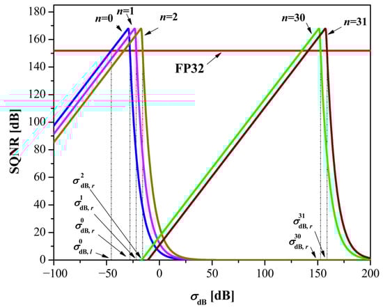
Figure 1.
SQNR as a function of σdB for the FXP32 format, for various n.
Lemma 1.
The SQNR curve of the FXP32 quantizer provided for n + 1 is 6.02 dB away from that provided for n, i.e.:
Proof of Lemma 1.
According to (13) we have
Note that 2 = 106.02/20 and 22 = 106.02/10, so expression (15) becomes
which completes the proof. □
Let us denote with the variance where the SQNR curve for a given n reaches its maximum. This important parameter for further analysis will be determined iteratively, as Lemma 2 shows.
Lemma 2.
The point
at which the SQNR of the FXP32 quantizer provides the maximum can be specified by
Proof of Lemma 2.
Let us define function S as follows:
Using the condition , we get the following identity:
Finally, solving (19) by we have
The last equation can be solved iteratively, and the proof is finished. □
The iterative process (17) can be initialized with , where C = 151.9 dB is the SQNR score of the FP32 format [13], which will also be used during the performance comparison process, as shown below.
By observing a certain value of n, Figure 1 shows a rapid decrease in SQNR when moving away (left and right) from the point . This means that FXP32 is not robust to changes in the variance level (robustness is essential for processing variance-sensitive data). On the other hand, this is not the issue for the FP32 format, which maintains a stable SQNR over a wide variance range. By directly comparing the achieved SQNR values, it can be seen that the FXP32 is able to achieve better scores than FP32 but only in a small range of σdB values. This means that FXP32 can represent data with a higher precision than FP32 within a narrow variance range; hence, it is a great option for data that exhibits low variance range. However, practical applications (e.g., neural networks) typically require a much wider variance range, and improving the FXP32 format is essential for effective use.
By increasing the SQNR in the wide variance range, this work achieves an extension of the FXP32 format’s dynamic range. The method exploits the switching strategy [15] but applies different design criteria, as will be explained in the next section.
3. Switched FXP32 Format
This section presents a switched FXP32 format that uses a range of possible n values, in contrast to the classic FP32 format, where n is fixed. Each n can operate within a certain range of variances while the data variance level defines which one will be chosen (i.e., switching is accomplished variance-wise). Thus, switched FP32 allows partitioning the variance range into non-overlapping ranges and assigns the optimal n to each range. The identification of non-overlapping variance ranges, also known as subranges, is an essential task. The process applied here is distinct from that in [15], where the intersection points of the SQNR curves of neighboring n are used as subrange boundaries. This will be clarified next.
The design of the considered solution seeks to achieve the SQNR performance for each n equal to or higher than the FP32, which can be mathematically formulated as follows:
where and represent the lower and upper bound of the subrange (n in the superscript refers to n value), where 0 ≤ n ≤ 31. Clearly, we set const. = C = 151.9 dB.
We will use Figure 1 to explain the division of the variance range considering criterion (21). Note that the SQNR curve of the classic FXP32 format for each observed n intersects the SQNR curve of the FP32 format at two variance points, left and right from , denoted as and , respectively. Thus, a general rule for creating non-overlapping subranges is introduced:
- Select as the upper bound, i.e., , 0 ≤ n ≤ 31;
- Select the upper bound for the pervious n as the lower bound for the current n, i.e., , 1 ≤ n ≤ 31, except for the case n = 0, where .
To determine an iterative rule is proposed, as Lemma 3 indicates.
Lemma 3.
The upper threshold of the subrange corresponding to n can be found with the following iterative rule:
Proof of Lemma 3.
To prove this, we will use expression (12) and apply the following condition:
that is,
Solving (24) with respect to , we obtain the following equation:
which requires iterative solving, so the proof is completed. □
The appropriate initialization of (22) can be achieved with , where is defined with (17).
Given that is a critical parameter, this paper proposes a very accurate approximate expression for its calculation. According to Figure 1, the SQNR decreases for because the component Dov has a greater effect on the total distortion than Dg. Therefore, the SQNR can be approximated as follows:
Now, the approximate , denoted as , can be obtained as the solution of the following equation:
resulting in
The relative error calculated for n ranging from 0 to 31 is illustrated in Figure 2. It is obvious that the approximate formula (28) is very accurate, with an approximation error below 0.2%.
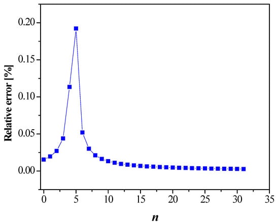
Figure 2.
Relative error for the approximate upper bound defined by (28).
The switched FXP32 format can be described following the subranges’ determination. The principle of work depends on whether the input data has a zero or non-zero mean, as shown in Figure 3. Let xi, i = 1, 2,…, M, denote the input data samples. The mean µ can be calculated as follows [16]:
If µ = 0, then the variance of the data should be estimated as follows [16]:
which is further used to select n for available data according to the following:
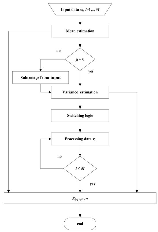
Figure 3.
The flowchart of the proposed switched FXP32 format.
Since n is required in the decoding phase, it should be quantized and stored in the memory using 32 bits. After this, data samples are simultaneously processed using (4), and the quantized data xi,q are obtained. When µ ≠ 0, the aforementioned steps must be applied after subtracting the mean from the input data. In this scenario, 32 bits should be used to quantize and store µ in the memory. In the decoding phase, for zero-mean data, decoding samples are xi,d = xi,q, while in the other case, xi,d = xi,q + µ. Algorithm 1 shows the algorithm for switched FXP32 quantization of input data for a more detailed explanation.
| Algorithm 1: The switched FXP32 quantization procedure |
| (n = 0, …,31) % Encoding phase 1: Estimate mean µ using (29) 2: if µ ≠ 0 then 3: Subtract µ from input data 4: end if 5: Calculate variance σ2 using (30) 6: Apply the switching logic (31) to select n; 7: while i ≤ M do 8: Process data using (4) to obtain quantized samples xi,q 9: end while % Decoding phase Require: quantized data samples xi,q (i = 1,…,M), n, µ 1: while i ≤ M do 2: if µ = 0 then 3: Decode data as xi,d = xi,q 4: else 5: Decode data as xi,d = xi,q + µ 6: end if 7: end while |
The SQNR will also be used to express the performance of the switched FP32 format. It can be derived from the classic FXP32 format’s SQNR utilizing the portions of the curves inside the subrange borders, as expected:
4. Results and Discussion
This section presents the theoretical performance (SQNR) results for the proposed switched FXP32, together with the experimental and simulation results based on real data.
4.1. Theoretical SQNR Results
Figure 4 illustrates the theoretical SQNR for the switched FXP32. It indicates subranges where certain n performs, while the boundaries of these subranges are also determined and reported in Table 1. Figure 4 also shows other relevant parameters, such as the dynamic range limits and , the minimum and maximum values of SQNR, and the SQNR dynamics = − . In addition, δn is also indicated, which denotes the width of the subrange. Note that each subrange, except the one where n = 0 is assigned, has a constant width of 6.02 dB (this can also be concluded from Table 1). The concrete numerical values of these parameters are listed in Table 2.
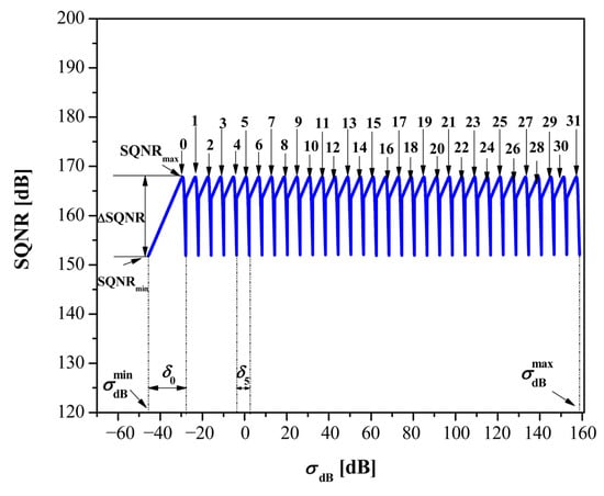
Figure 4.
SQNR of the switched FXP32 format across a wide range of variances.

Table 1.
The values of subrange threshold .
Table 2.
The values of specific parameters of the switched FXP32.
Comparison with fixed-point baselines. As fixed-point baselines, we use the DFP and S-DFP formats [6]. Both DFP and S-DFP use r = 8 bits for the integer part and an 8-bit shared exponent. For DFP8, the shared exponent is given by es = em − (r − 2), where em = is the exponent of the absolute maximum data value, while its step size is ∆DFP = . In the case of S-DFP8, the step size is ∆S-DFP = , where em_mod = em − bias − (r − 2) is the shared exponent and bias = 8. The performance for DFP8 and S-DFP8 formats can be calculated using (6), (7), and (11), assuming that and , and the results are presented in Figure 5 and Figure 6, respectively, for several values of σdB. Figure 5 reveals that DFP8 heavily depends on em for a particular data variance. Note that the optimal em for some variance (e.g., em = 0 for σdB = −10 dB) does not guarantee the maximal SQNR (nearly 35 dB [16]) of the DFP8 format across other variances. So, the rule above for em will provide an optimal choice for some variance, but in most cases, it will differ from the actual variance of the data. Nevertheless, even if the optimal em is chosen, the capabilities of DFP8 are significantly below the proposed switched FXP32 for the same variance values (see Figure 4).
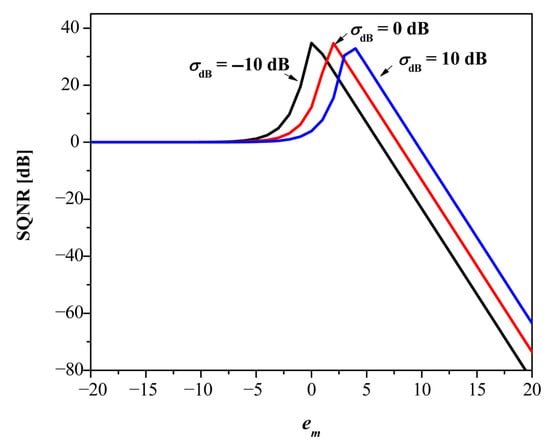
Figure 5.
SQNR vs. em for DFP8 for several data variance values.
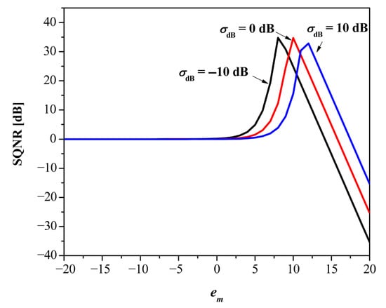
Figure 6.
SQNR vs. em for S-DFP8 for several data variance values.
It is easy to see that the SQNR of the S-DFP8 format is a shifted version of the SQNR of the DFP8, so the conclusions drawn above can be extended to S-DFP8.
Comparison with floating-point baselines. As floating-point baselines, we use the FP32 [13] and bfloat16 [18] formats, as shown in Figure 7.
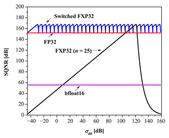
Figure 7.
Comparison of the switched FXP32 with different floating-point solutions.
In the provided figure, we have also added the SQNR curve of the classic FXP32 format, whose key parameter is selected in the following way:
where m = 3000 is the number of variances σj from the range [,]. In other words, within a given variance range, such n should provide the best performance in terms of average SQNR (SQNRav). Figure 8 reveals that n = 25 satisfies the condition (33).
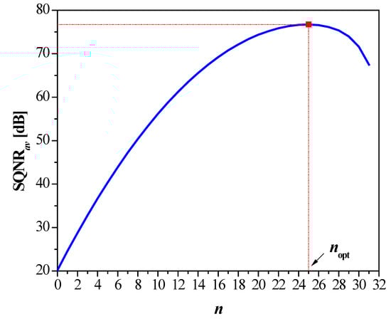
Figure 8.
The average SQNR versus n for the classic FXP32 format.
It is obvious from Figure 8 that the classic FXP32 (n = 25) enables the same maximal SQNR, but it works in a much lower dynamic range with respect to our proposal (16.1 dB vs. 204.3 dB). The included floating-point baselines provide a stable SQNR in the observed variance range, with FP32 achieving the best scores. Interestingly, the classic FXP32 allows for better SQNR across a relatively wide variance range with respect to the bfloat16 format. Compared to FP32 and bfloat16, the switched FXP32 format enables a competitive dynamic range, with gains in maximum SQNR of 15.9 dB and 112.2 dB, respectively. This confirms the high efficiency of the proposed solution.
4.2. Experimental SQNR Results
The experimental part is based on weights obtained from several NN configurations and databases. The networks MLPI (multi-layer perceptron) and CNNI (convolutional neural network) are applied to the MNIST database [19], while more complex MLPII and CNNII are applied to the CIFAR-10 database [20].
MLPI uses one hidden layer with 128 nodes, while its input and output layers use 784 and 10 nodes, respectively. The activation functions used in the hidden and output layers are ReLU and softmax, respectively. Hyper parameters are adopted following values regularization rate = 0.3, learning rate = 0.0005, and batch size =128. Training is performed over 50 epochs.
For CNNI we adopt the model in [12], which incorporates convolutional, max pooling, a fully connected layer, and an output layer. The number of output filters in the convolutional layer is set to 32, while its kernel size is 3 × 3. The size of the pooling window is 2 × 2. The fully connected layer with 100 units on top of it, which is activated by the ReLU activation function, is placed further, before the output layer. Dropout of 0.5 is performed on the fully connected layer. CNNI is trained in batches of size 128 across 10 epochs.
MLPII comprises five fully connected hidden layers with progressively decreasing dimensionality: two layers with 512 units, followed by two with 256 units, and one with 128 units. These are followed by a final output layer that predicts probabilities across the ten CIFAR-10 classes. To improve training dynamics and reduce overfitting, the architecture includes batch normalization (to stabilize and accelerate training) and dropout (as a form of regularization). Data augmentation is applied during training in the form of random cropping and horizontal flipping, while validation and test data are standardized using only pixel-wise normalization. The network is trained for 40 epochs using the Adam optimizer with a learning rate of 0.0001.
CNNII architecture follows a VGG-style design composed of three convolutional blocks. Each block contains two convolutional layers with ReLU activations and same-padding, followed by batch normalization to improve stability, max pooling for spatial down sampling, and dropout for regularization. The number of convolutional filters increases across blocks, from 64 to 128 and, finally, to 256. A fully connected stage with 512 units follows the convolutional blocks, again incorporating batch normalization and dropout. The network is trained for 30 epochs using the Adam optimizer with a learning rate of 0.001.
The weight histograms of the trained MLP and CNN networks are depicted in Figure 9. Observe that the distribution of weights can be approximated using a Laplacian PDF (especially for Figure 9a–c). The existence of Laplacian data in NNs is therefore well validated. For MLPI we used the weights between the input and hidden layer (100,352 in total), whose variance is σw2 = 5.77 × 10⁻⁴ (σw,dB = −32.39 dB) (Figure 9a). In the case of CNNI, we analyzed the weights between the input and hidden layer in the fully connected part (540,800 in total), whose variance is σw2 = 0.0034 (σw,dB = −24.67 dB) (Figure 9b). The weights in MLPII are from the first fully connected layer (1,572,864 in total) whose variance is σw2 = 6.84 × 10⁻⁴ (σw,dB = −31.65 dB) (Figure 9c). Finally, from CNNII we also employ the weights from the fully connected part (2,097,152 in total), having a variance of σw2 = 0.0079 (σw,dB = −21 dB) (Figure 9d). All the weight sets used have a mean value close to zero.
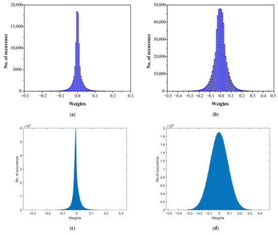
Figure 9.
Histograms of weights of trained neural networks: (a) MLPI (MNIST database); (b) CNNI (MNIST database); (c) MLPII (CIFAR-10 database); (d) CNNII (CIFAR-10 database).
Table 3 gives the experimental SQNR for the proposed FP32 and DFP8 [6] approaches, calculated as follows [12]:
where wi denotes the unquantized weight, wi,q is the quantized weight, and M is the total number of weights. It is evident that the capability of the proposed switched FXP32 on the weights of all the considered MLP/CNN architectures is higher than that of the employed baselines. Note that even in a case that has a slightly different distribution (CNNII weights) and, therefore, suboptimal optimization, evidence suggests that there are still improvements. For identical variance values, the achieved experimental SQNR results are in very good agreement with the theoretical ones displayed in Figure 7.
Table 3.
Experimental SQNR for the switched FXP32, FP32, and DFP8 [6], obtained on weights from different NN architectures.
4.3. Simulation SQNR Results
The simulation part uses the weights from the experimental part (e.g., from the MLPII network) as starting points and aims to verify the efficiency of the switched FXP32 format in situations where the variance of the weights changes. Figure 10 demonstrates the simulation SQNR for weights with variance in the range of −40 dB to 150 dB, provided using the following procedure:
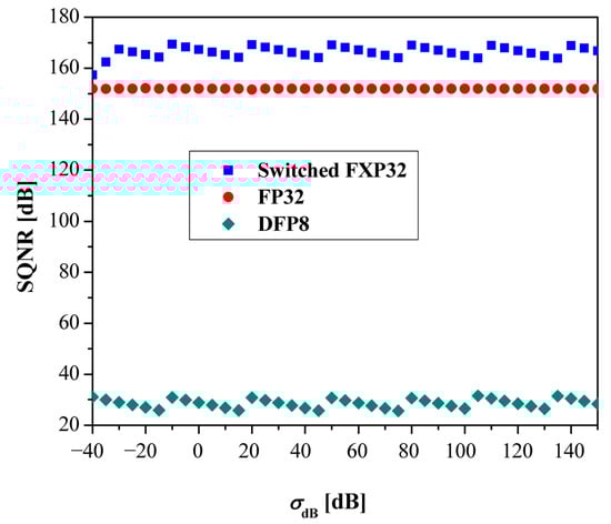
Figure 10.
SQNR simulation results obtained for the weights of the MLPII network.
- (1)
- Scale the initial weights with to obtain the new weights of variance σdB;
- (2)
- Apply Algorithm 1 (Section 3) on the new weights;
- (3)
- Calculate SQNR using (34).
Note that the switched FXP32 format preserves high SQNR values and outperforms the FP32 and DFP8 formats [6], while the simulated SQNR aligns well with the theoretical SQNR shown in Figure 7. This confirms the correctness of the theoretical design method. The fact that this approach achieves high efficiency in encoding various Laplacian-distributed data is a strong indicator of its potential usefulness in neural network applications.
4.4. Limitations
Although our method is effective, it exhibits certain shortcomings. Encoding data with variance outside its dynamic range may be less efficient compared to FP32. As a mitigation measure, a scaling method can be applied to shift the variance of the data into the desired range and return the data with rescaling at the end.
5. Conclusions
An effective method for improving the FXP32 format for the Laplacian-distributed data was presented in this paper. Its main attribute is the ability to vary the number of bits for the integer part (denoted by n) depending on the estimated variance of the input data, unlike the classic FXP32 format, where this parameter is fixed. Due to the calculation of external parameters, a slightly increased computational complexity was introduced compared to the classic variant. The theoretical design process was comprehensively explained, and the critical parameters were determined along with the expression for performance evaluation. Theoretical analysis over a wide variance range was performed using SQNR as a performance metric, revealing a significant gain over existing floating-point (e.g., standardized FP32) and fixed-point baselines. The experimental and simulation analysis based on neural network weights were further included to validate the theoretical results. Based on these encouraging findings, we believe that the presented switched FXP32 can be a useful solution in real-world systems where Laplacian-distributed data occurs, e.g., neural networks. Moreover, future work will include the application in neural networks as an alternative to FP32, where considerable savings in computational and hardware resources are expected.
Author Contributions
Conceptualization, B.D. and Z.P.; methodology, B.D. and Z.P.; software, B.D., M.D., N.S. and M.A.; validation, B.D., Z.P. and M.D.; investigation, B.D., Z.P., M.D. and S.P.; resources, M.D.; data curation, S.P., N.S. and M.A.; writing—original draft preparation, B.D.; writing—review and editing, Z.P. and M.D.; visualization, B.D. and M.D.; supervision, Z.P. All authors have read and agreed to the published version of the manuscript.
Funding
This work was supported by the Ministry of Science, Technological Development and Innovation of the Republic of Serbia (grant number 451-03-136/2025-03/200102), as well as by the European Union’s Horizon 2023 research and innovation program through the AIDA4Edge Twinning project (grant ID 101160293).
Institutional Review Board Statement
Not applicable.
Informed Consent Statement
Not applicable.
Data Availability Statement
The data presented in this study are available on request from the corresponding author.
Conflicts of Interest
The authors declare no conflicts of interest.
Abbreviations
The following abbreviations are used in this manuscript:
| bfloat16 | Brain floating-point format |
| CIFAR-10 | Canadian Institute for Advanced Research database |
| CNN | Convolutional neural network |
| DFP | Dynamic fixed-point format |
| FP | Floating point |
| FP32 | 32-bit floating-point format |
| FXP | Fixed-point format |
| FXP32 | 32-bit fixed-point format |
| MNIST | Modified National Institute of Standards and Technology database |
| MLP | Multilayer perceptron |
| MSE | Mean squared error |
| NN | Neural network |
| Probability density function | |
| S-DFP | Shifted dynamic fixed-point format |
| SQNR | Signal to quantization noise ratio |
References
- IEEE 754-2019; Standard for Floating-Point Arithmetic. IEEE: Piscataway, NJ, USA, 2019. [CrossRef]
- Mienye, I.D.; Swart, T.G.; Obaido, G. Recurrent neural networks: A comprehensive review of architectures, variants, and applications. Information 2024, 15, 517. [Google Scholar] [CrossRef]
- Aymone, F.M.; Pau, D.P. Benchmarking in-sensor machine learning computing: An extension to the MLCommons-Tiny suite. Information 2024, 15, 674. [Google Scholar] [CrossRef]
- He, F.; Ding, K.; Yan, D.; Li, J.; Wang, J.; Chen, M. A novel quantization and model compression approach for hardware accelerators in edge computing. Comput. Mater. Contin. 2024, 80, 3021–3045. [Google Scholar] [CrossRef]
- Das, D.; Mellempudi, N.; Mudigere, D.; Kalamkar, D.; Avancha, S.; Banerjee, K.; Sridharan, S.; Vaidyanathan, K.; Kaul, B.; Georganas, E.; et al. Mixed precision training of convolutional neural networks using integer operations. arXiv 2018, arXiv:1802.00930. [Google Scholar]
- Sakai, Y.; Tamiya, Y. S-DFP: Shifted dynamic fixed point for quantized deep neural network training. Neural Comput. Appl. 2025, 37, 535–542. [Google Scholar] [CrossRef]
- Kummer, L.; Sidak, K.; Reichmann, T.; Gansterer, W. Adaptive Precision Training (AdaPT): A Dynamic Fixed Point Quantized Training Approach for DNNs. In Proceedings of the 2023 SIAM International Conference on Data Mining (SDM23), Minneapolis, MN, USA, 27–29 April 2023. [Google Scholar] [CrossRef]
- Alsuhli, G.; Sakellariou, V.; Saleh, H.; Al-Qutayri, M.; Mohammad, B.; Stouraitis, T. DFXP for DNN architectures. In Number Systems for Deep Neural Network Architectures: Synthesis Lectures on Engineering, Science, and Technology; Springer: Cham, Switzerland, 2024. [Google Scholar] [CrossRef]
- Sungrae, K.; Hyun, K. Zero-centered fixed-point quantization with iterative retraining for deep convolutional neural network-based object detectors. IEEE Access 2021, 9, 20828–20839. [Google Scholar] [CrossRef]
- Wu, S.; Li, G.; Chen, F.; Shi, L. Training and inference with integers in deep neural networks. arXiv 2018, arXiv:1802.04680. [Google Scholar]
- Banner, R.; Nahshan, Y.; Hoffer, E.; Soudry, D. ACIQ: Analytical clipping for integer quantization of neural networks. arXiv 2018, arXiv:1810.05723. [Google Scholar]
- Peric, Z.; Savic, M.; Simic, N.; Denic, B.; Despotovic, V. Design of a 2-bit neural network quantizer for Laplacian source. Entropy 2021, 23, 933. [Google Scholar] [CrossRef] [PubMed]
- Peric, Z.; Savic, M.; Dincic, M.; Vucic, N.; Djosic, D.; Milosavljevic, S. Floating Point and Fixed Point 32-bits Quantizers for Quantization of Weights of Neural Networks. In Proceedings of the 12th International Symposium on Advanced Topics in Electrical Engineering (ATEE 2021), Bucharest, Romania, 25–27 March 2021. [Google Scholar] [CrossRef]
- Peric, Z.; Dincic, M. Optimization of the 24-Bit fixed-point format for the Laplacian source. Mathematics 2023, 11, 568. [Google Scholar] [CrossRef]
- Dincic, M.; Peric, Z.; Denic, D.; Denic, B. Optimization of the fixed-point representation of measurement data for intelligent measurement systems. Measurement 2023, 217, 113037. [Google Scholar] [CrossRef]
- Jayant, N.C.; Noll, P. Digital Coding of Waveforms: Principles and Applications to Speech and Video; Prentice Hall: Englewood Cliffs, NJ, USA, 1984. [Google Scholar]
- Gersho, A.; Gray, R. Vector Quantization and Signal Compression; Kluwer Academic Publishers: New York, NY, USA, 1992. [Google Scholar]
- Burgess, N.; Milanovic, J.; Stephens, N.; Monachopoulos, K.; Mansell, D. Bfloat16 Processing for Neural Networks. In Proceedings of the IEEE 26th Symposium on Computer Arithmetic (ARITH 2019), Kyoto, Japan, 10–12 June 2019. [Google Scholar] [CrossRef]
- Lecun, Y.; Cortez, C.; Burges, C. The MNIST Handwritten Digit Database. Available online: http://yann.lecun.com (accessed on 1 February 2025).
- Krizhevsky, A.; Nair, V. The CIFAR-10 and CIFAR-100 Dataset. 2019. Available online: https://www.cs.toronto.edu (accessed on 1 February 2025).
Disclaimer/Publisher’s Note: The statements, opinions and data contained in all publications are solely those of the individual author(s) and contributor(s) and not of MDPI and/or the editor(s). MDPI and/or the editor(s) disclaim responsibility for any injury to people or property resulting from any ideas, methods, instructions or products referred to in the content. |
© 2025 by the authors. Licensee MDPI, Basel, Switzerland. This article is an open access article distributed under the terms and conditions of the Creative Commons Attribution (CC BY) license (https://creativecommons.org/licenses/by/4.0/).