Research on Resource Allocation Algorithm for Non-Orthogonal Multiple Access Backscatter-Based Cognitive Radio Networks

Abstract

Integrating Non-Orthogonal Multiple Access (NOMA) backscatter with Cognitive Radio (CR) can effectively alleviate the pressure of large-scale Internet of Things (IoT) device connections while reducing power consumption. In the downlink of NOMA backscatter-based CR networks (NB-CR), most researchers only consider the case of a single backscatter device (BD), ignoring the fact that multiple BDs can prolong device usage and enhance system robustness. The resource allocation (RA) problem is crucial in the downlink of NB-CR networks. Most existing RA algorithms focus on system throughput but rarely consider energy efficiency (EE). In this paper, we propose the RA problem for downlink communication (NBCR-RA) in NB-CR networks with multiple BDs. We jointly optimize power allocation coefficients and reflection coefficients (RCs) to maximize EE. We model the NBCR-RA problem as a non-convex problem and divide it into two subproblems: power allocation optimization and RC optimization. Firstly, we propose a Lagrange-based power allocation optimization (L-PA) algorithm to obtain the optimal power allocation coefficients. Secondly, we design an RC optimization algorithm, PS-RC, based on a particle swarm algorithm to determine the optimal RCs. Finally, we validate the superiority of L-PA and PS-RC algorithms in terms of EE. Through multiple experiments, we obtained a $95\%$ confidence interval of [10.5552, 10.6465].

1. Introduction

With the continuous increase in IoT users, the connection of large-scale IoT devices has become a trend. The combination of NOMA and CR can effectively alleviate the pressure caused by massive connections. NOMA technology enables the transmission of multi-user data within the same frequency band, dynamically allocating spectrum based on the needs and channel conditions of different users. CR dynamically adjusts the access power of secondary users based on the activity of the primary user, achieving multi-user access [1]. With the development of the green IoT [2], people are increasingly concerned about energy consumption issues while considering data rates. The concept of energy efficiency can be proposed to consider both user rates and system energy consumption.

In NOMA backscatter networks, the RA problem is a crucial issue that affects the quality of communication. In papers [3,4], a NOMA backscatter network was proposed, consisting of one BS, one BD, and two users for communication. The RA problem was studied under this model. However, the previous research only considered the case of BD and ignored some real-life situations. In situations involving remote or difficult-to-replace equipment, deploying multiple BDs can extend the service life of the system, enhance the robustness of the entire communication system, and prevent system failure due to the malfunction of a single BD. Therefore, it is necessary to study the NOMA backscatter network of multiple BDs. In paper [5], although multiple-BDs NOMA backscatter networks were studied, only the throughput of users was considered, lacking consideration for the overall EE of the system.

In paper [6], although the RA problem in NOMA backscatter networks with multiple BDs was studied and the energy consumption of the system was considered, the research mainly focused on the uplink. In the paper [7], a NOMA backscatter CR uplink network was proposed. In this communication network model, the goal is to maximize throughput, based on the Concave Convex Process (CCCP), and an optimal solution is obtained through iteration. In communication networks, to meet the data transmission needs of different users, it is important to transmit data from the base station (BS) to users through the downlink. Therefore, this paper studies the RA problem in the downlink of NOMA backscatter-based CR networks and considers EE as the optimal objective.

In this article, we propose an NOMA backscatter-based CR network to meet the constraint on the interference of the secondary transmitter (ST) on the primary user (PU). The network consists of one BS, two users, and multiple BDs. BDs not only perform energy harvesting (EH) in this network model but also backscatter the received signals. To achieve this, we have adopted a time slot-based EH method. To reduce energy consumption while ensuring user data rate, we propose the NBCR-RA problem with EE as the optimization objective that satisfies QoS conditions. This problem jointly optimizes the power allocation coefficient and RC. To solve this non-convex problem, we divide it into two optimization subproblems. We prove that the first optimization subproblem is convex and use the L-PA algorithm to obtain the optimal power allocation coefficient. Based on the solution of the first optimization subproblem, we can obtain the relationship between RC and the power allocation coefficient. For the second optimization subproblem, we solve it through the PSO algorithm to obtain the optimal RC.

From the problems mentioned above, we propose an RA algorithm for multiple BDs to solve the NBCR-RA issues. The contributions are described as follows:

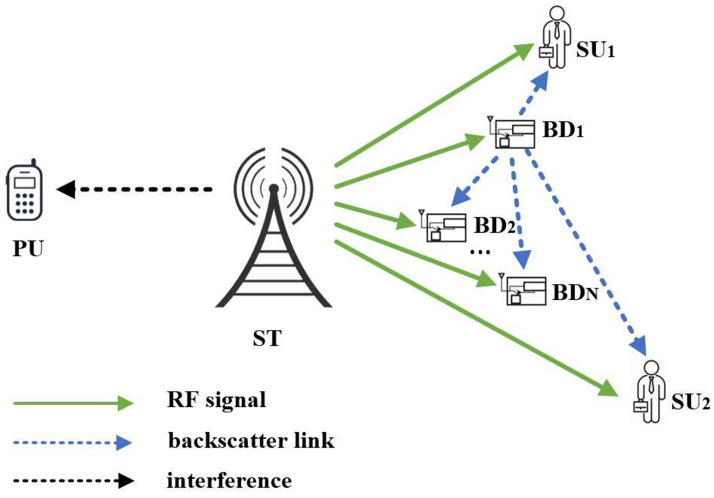
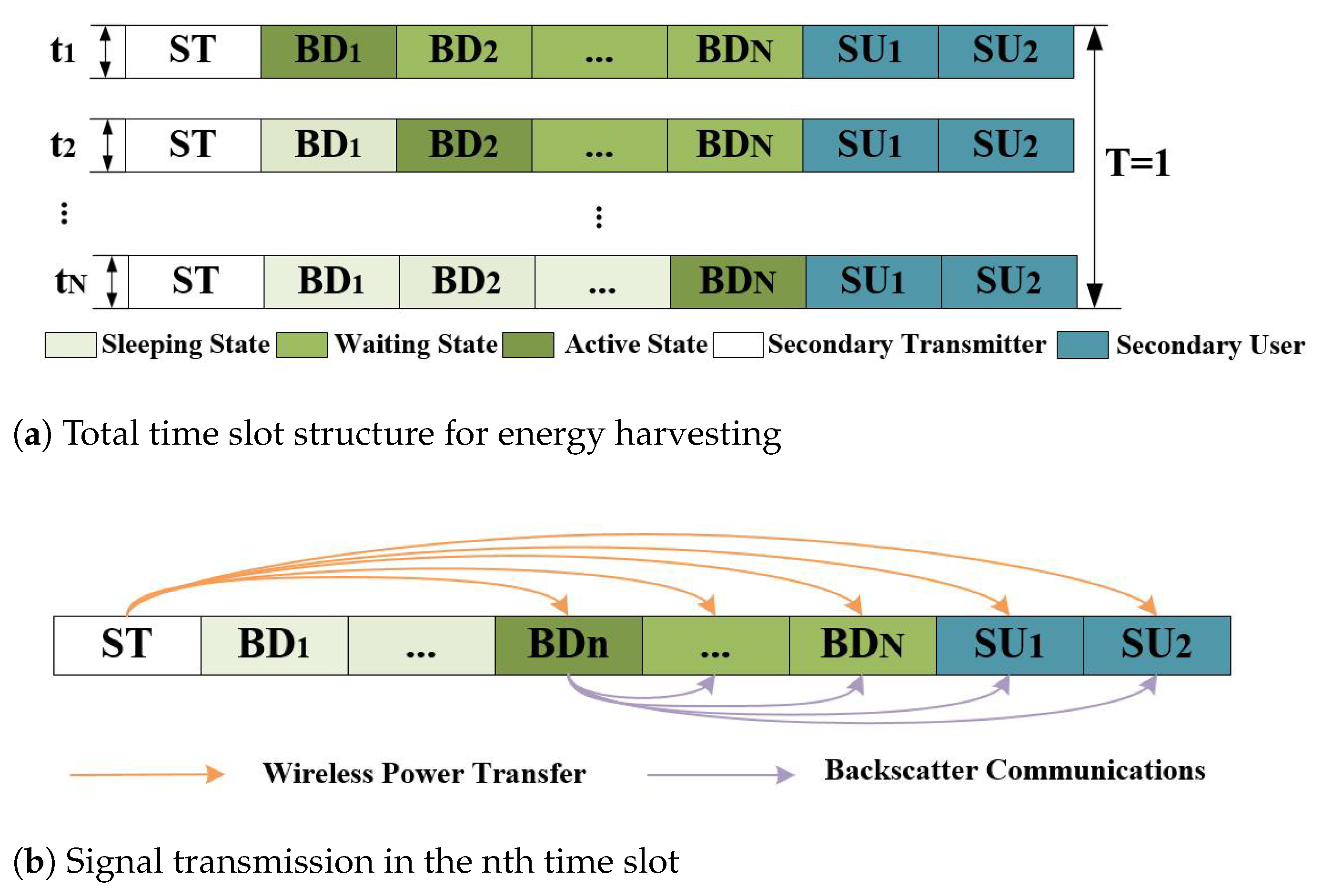
• An NB-CR network is proposed, which contains multiple BDs and two NOMA users. In this network, ST communicates with secondary users (SUs) based on NOMA technology and BDs use a timeslotted method for EH and backscatter communication.
• We formulate an NBCR-RA problem with EE as the optimization objective. We prove that the problem is non-convex and divide it into two subproblems.
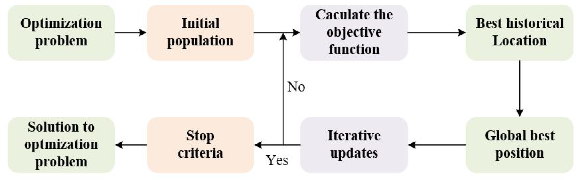
• We design an L-PA algorithm for the first subproblem. This algorithm uses Lagrange and subgradient iterative optimization algorithms to solve the power allocation subproblem. For the second subproblem, we design a PS-RC algorithm to search for the optimal RCs.
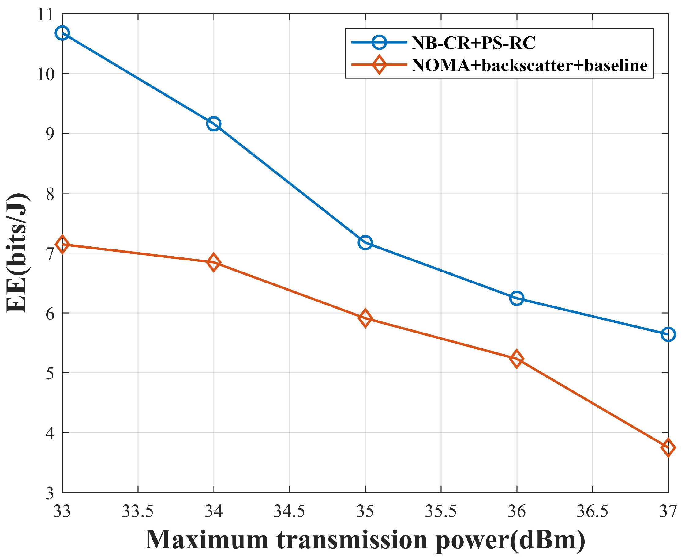
• For comparison, we introduce several baseline models. We compare the performance of the algorithm presented in this article with the traditional power allocation algorithms under different models through simulation experiments to validate the superiority of the algorithm proposed in this article.

2. Related Work

The RA problem is an important issue in NOMA backscatter networks, as it directly impacts communication quality. In paper [8], a NOMA-based CR network is proposed, ensuring that the interference to PU remains within an acceptable range. This network uses simultaneous wireless information and power transfer (SWIPT) technology, transmitting information through coverage and underlying modes. On the basis of this network, a problem aimed at maximizing sum rate is proposed, along with a binary algorithm is proposed to solve the optimal power allocation coefficient and perception time coefficient. In paper [9], the problem of jointly optimizing the power allocation coefficient and RC with the objective of maximizing system EE in the NOMA backscatter network is proposed. To solve this problem, the authors use the Dinkelbach method, decoupling it into two subproblems: the optimal transmission power subproblem and the optimal RC subproblem. The solution is then obtained using duality theory, Karush-Kuhn-Tucker (KKT) conditions, and a subgradient iterative algorithm. These studies highlight the significance of the RA problem in enhancing system performance and user experience in NOMA backscatter networks.

In the NOMA backscatter network, the BS sends signals to two users and one BD, which acts as a relay. Paper [10] maximizes the EE of users under constraints such as Signal-to-Interference-plus-Noise Ratio (SINR) requirements and transmission power. To solve the RA problem, this paper proposes an iterative method based on Dinkelbach. Paper [9] proposes an NOMA backscatter-based CR network, which also contains only one BD in the network and calculates the size of EE. In reality, to ensure the service life and robustness of the system, multiple BDs will have more advantages than one BD.

In paper [11], a typical NOMA backscatter-based CR model is proposed, incorporating multiple BDs. This model enables backscattering communication based on time-division multiple access (TDMA) and active transmission based on NOMA. The main objective of this article is to maximize the throughput of system. To this end, the problem is first represented as a Markov decision process and solved through deep learning. In paper [10], a hybrid relay network for power domain NOMA backscatter is proposed, which includes multiple BDs. They first collect energy and decode information, and then forward the data to the receiver simultaneously based on NOMA. To find the optimal RA solution and reduce complexity, it is divided into two subproblems to solve. In paper [7], the main focus is on an NOMA backscatter-based CR network with multiple BDs, where the goal is to maximize the total rate of users under causal constraints of multi-slot energy. The solution involves calculating the maximum sum rate for a given RC and transmission power. In paper [11], a multi-BD dual base NOMA backscatter network is proposed. To maximize the throughput of all BDs, this paper adopts convex optimization methods and proposes an iterative algorithm to solve the optimal solution. The above paper only considered the throughput during the research process and did not take into account the energy consumption of the system.

In the paper [6], an NOMA backscatter uplink network is proposed, which differs from previous works. The BDs not only obtain energy from the BS but also collect energy from BDs that have previously backscattered. In order to achieve maximum EE, this paper combines RC, transmission time, and beamforming for optimization. In this network, multiple aspects such as the causality of EH and constraints on throughput are considered simultaneously. Under these constraints, a non-convex problem is formulated. The Dinklebach method is used to transform the form and iteratively solve the corresponding optimal solution. However, the research mainly focuses on the uplink. In fact, due to varying data requirements of different users, downlink communication is also necessary. This article mainly studies multiple-BD CR networks based on NOMA backscatter.

3. System Model and RA Problem Formulation

3.1. System Model

We propose an NB-CR network presented in Figure 1. We assume that the ST, BDs, and users are provided with a single antenna, and all channel models follow independent Rayleigh distribution [12]. The network model is divided into primary and secondary networks. The primary network mainly contains the PU, which is mainly affected by interference from the ST. The secondary network contains the ST, two SUs, and N BDs.

The single-antenna ST transmits superposition signals for the two SUs based on NOMA technology and the signals to the BDs. Part of the signals received by the BDs is used for EH to support their circuit operation, and part for backscatters [13]. The BDs modify the received signals and reflect them towards $S{U}_1$, $S{U}_2$, and the rest of the BDs. Thus both $S{U}_1$ and $S{U}_2$ receive information from the ST and the BDs [14]. $S{U}_1$ and $S{U}_2$ decode signals based on successive interference cancellation (SIC) techniques.

In Figure 1, $h_{s{u}_1}(n)$, $h_{s{u}_2}(n)$, $h_{s{b}_n}(n)$, $h_{b_n{u}_1}(n)$, $h_{b_n{u}_2}(n)$, $h_{SR}(n)$, and $h_{b_i{b}_n}(n)$ denote the channels between ST to $S{U}_1$, ST to $S{U}_2$, ST to $B{D}_n$, $B{D}_n$ to $S{U}_1$,$B{D}_n$ to $S{U}_2$, ST to PU, and the i-th BD to the n-th BD, respectively, all of which conform to the complex Gaussian distribution, i.e., $h_j(n)\sim CN(0,{\lambda }_k)$, $j\in (s{u}_1,s{u}_2,s{b}_n,b_n{u}_1,b_n{u}_2,SR,b_i{b}_n)$, $k\in (1,2,3,4,5,6,7)$ [15]. The corresponding channel gains are expected to be constant over a time interval and they are denoted by $d^{(-\alpha )}$, where $\alpha$ indicates the path loss exponent and d indicates the distance between nodes. The magnitude of path loss is related to the distance of signal transmission, and the formula is $PL(d)=PL(d_0)+10\alpha lo{g}_{10}({\displaystyle \frac{d}{d_0}})$ [2]. In this equation, $d_0$ is the reference distance and $PL(d_0)$ represents the path loss at the reference distance $d_0$. Considering the outdoor environment, the path loss index can be set to 3 [4,6,16]. As the transmission power increases, the received power also increases correspondingly.

In this paper, we adopt the method in paper [6] for EH. The ST uses TDMA technology to allocate time slots for each BD to backscatter, ensuring that each BD knows when it should backscatter. The specific frame structure is depicted in Figure 2. In Figure 2a, the frame duration T is standardized to 1, with each time slot having a duration of 1/N. The first BD contains two states: active and sleeping. The n-th BD also contains two states: active and waiting. The remaining BDs possess three states: active, waiting, and sleeping. When a BD is backscattering, it is in the active state. If a BD has not completed backscattering, it is in the waiting state. Once a BD completes its backscatter during its time slots, the ST will no longer send signals to the BDs. Additionally, the backscattered signals from the BDs are too weak to reach the threshold of EH and the threshold of signal reception. So, at this point the BDs neither backscatter nor harvest energy, entering the sleeping state. Figure 2b mainly depicts the signal transmission of the entire system at the n-th time slot.

3.2. Energy Harvesting and Consumption

In CR networks, there is some interference from the secondary network to the primary network. To protect the information transmission of PUs, PUs impose strict interference constraints on the ST [12,17]. The interference allowed at a PU is represented by $PI$, and $P_{sb}$ denotes the maximum transmit power of the ST. Under underlay constraint cognizance, the transmit power of the ST is satisfied:

$$Ps=min(P_{sb},{\displaystyle \frac{PI}{|h_{SR}{|}^2}})$$

(1)

$$EH(n)=\beta (t|h_{s{b}_n}{|}^{2}Ps(1-r_n)+(n-1)t|h_{s{b}_n}{|}^{2}Ps+\sum _{i=1}^{n-1}t|h_{s{b}_i}{|}^{2}Ps{r}_i|h_{b_i{b}_n}{|}^2)$$

(2)

To better analyze the system in this article, in terms of EH, based on the papers [5,6], we adopted an approximate EH model to provide theoretical guidance for further research. Therefore, the collected energy can be represented by Equation (2) [16,18]. Equation (2) represents the energy harvested by the n-th BD in the n-th time slot. The harvested energy consists of three main components: the energy harvested from ST for the current time slot, the energy harvested from ST for the former (n − 1) time slots, and the energy harvested from the former (n − 1) BDs for the former (n − 1) time slots. In the equation, $\beta$ represents the energy transfer efficiency, and t expresses the period of the time slot in which the BD operates. We let $r\in R^{1\times N}$ denote the RCs of all the BDs, where $r=[r_1,r_2,\dots ,r_N]$, and $r_n$ denotes the RC of the n-th BD in the n-th time slot. All the $r_n\in [0,1]$.

From Equation (2), it can be seen that when $n=1$, the BD can only harvest energy at the current time slot. Therefore, we have $EH(1)=\beta t|h_{s{b}_n}{|}^{2}Ps{r}_n$.

When the received energy is too low, the sensitivity threshold of the EH is not reached. As more energy is harvested, the harvested energy can reach the saturation point $E{H}_{max}$. Thus, the harvested energy needs to satisfy

$$E{H}^{*}(n)=min(EH(n),E{H}_{max})$$

(3)

When n = 1, the harvested energy can be represented as $E{H}^{*}(1)=min(EH(1),E{H}_{max})$.

In addition, the total system energy consumption $Ec(n)$ for the n-th time slot can be represented as

$$Ec(n)=t(Ps+P_{bc})+(N-n)t{P}_{sc},$$

(4)

where $P_{bc}$ denotes the circuit energy consumption when BDs are backscattering. $P_{sc}$ represents the circuit energy consumption when BDs are in a waiting state. Both $P_{bc}$ and $P_{sc}$ include the circuit energy consumption of two SUs. The consumed energy $Ecc(n)$, excluding the power at the transmitter, is shown below:

$$Ecc(n)=t{P}_{b_c}+(N-n)t{P}_{s_c}$$

(5)

According to Equations (2) and (4), the accumulated energy of remaining BDs is higher and higher with increasing n, i.e., the more backward the sequence of BD, the more energy the BD collects. It is essential to strike a balance between accumulated energy and energy consumption.

3.3. NOMA Backscatter Communication

For the secondary network, the ST sends superposition information to two users at different levels of transmit power. At the n-th time slot, the ST transmits the signal [19]

$$x(n)=\sqrt{a_1(n)Ps}{x}_1(n)+\sqrt{a_2(n)Ps}{x}_2(n),$$

(6)

where $a_1\in R^{1\times N}$ and $a_2\in R^{1\times N}$ indicate the power allocation coefficients of $S{U}_1$ and $S{U}_2$, respectively. $a_1(n)$ and $a_2(n)$ indicate the power allocation coefficients at the n-th time slot and satisfy $a_1(n)+a_2(n)=1$ [20,21]. $x_1(n)$ and $x_2(n)$ stand for the information that the ST sends to $S{U}_1$ and $S{U}_2$, respectively, where $E[|x_1(n){|}^2]=1$, $E[|x_2(n){|}^2=1$.

The information of the BD is modulated to the main signal. At the n-th time slot, the signals received by the BD vary depending on its state. The n-th BD only receives the transmitted signal from the ST in the n-th time slot, while the BD that has backscattered no longer receives the signal. The BD that has not yet backscattered receives a combination of the signal transmitted by the ST and the signal backscattered by the n-th BD. Therefore, the signal received by a BD can be represented as follows [22]

$$y_{B{D}_i}(n)=\left\{\begin{array}{ccc}{h}_{s{b}_n}x(n)+n_0(n),\hfill & \hfill & i=n\hfill \\ h_{s{b}_i}x(n)+h_{s{b}_n}{h}_{b_i{b}_n}\sqrt{r_n}x(n)c(n)+n_0(n),\hfill & \hfill & i>n\hfill \end{array}\right.$$

(7)

where $n_0(n)$ denotes noise at $B{D}_n$ that obeys a circularly symmetric complex Gaussian distribution, i.e., $n_0(n)\sim CN(0,{\delta }^2)$. $c(n)$ represents the message of BD, where $E[|c(n){|}^2]=1$.

Assuming that the propagation delay at the BDs is negligible, the signal received at the $B{D}_n$ contains four components: the signal transmitted by the ST at the n-th time slot; the signal backscattered by the former (n − 1) BDs at the former (n − 1) time slots; the signal transmitted by the ST to the $B{D}_n$ at the former (n − 1) time slots; and Gaussian noise.

The signal received by $S{U}_1$ is divided into three sections: the signal sent by the ST to $S{U}_1$ in the current time slot, the signal backscattered by the BD to $S{U}_1$ in the current time slot, and noise. The received signal can be represented as

$$y(n)=h_{s{u}_1}x(n)+h_{s{b}_n}x(n)h_{b_n{u}_1}\sqrt{r_n}c(n)+n_1(n),$$

(8)

where $n_1(n)$ represents noise at $S{U}_1$ that obeys a circularly symmetric complex Gaussian distribution, i.e., the noise satisfies $n_1(n)\sim CN(0,{\delta }^2)$.

For the convenience of this study, it is assumed that the ST has access to the complete channel state information (CSI). The channel gain order is as follows: $|h_{s{u}_1}{|}^2>{|h_{s{u}_2}|}^2$. Each user will apply SIC techniques for signal decoding [3,7,23,24]. The sequence of SIC is obtained based on the sequence of channel gains. So, $S{U}_1$ can decode the signal of $S{U}_2$ first, i.e., $S{U}_1$ can decode the interference from the message of $S{U}_2$. The SINR [25] when $S{U}_1$ decodes its message can be depicted as

$${\gamma }_{1->1}(n)={\displaystyle \frac{a_1(n)Ps(|h_{s{u}_1}{|}^2+|h_{s{b}_n}{|}^2|h_{b_n{u}_1}{|}^2{r}_n)}{{\delta }^2}}$$

(9)

When $S{U}_2$ decodes its message, it treats the message of $S{U}_1$ as an interfering message, at which time the SINR is expressed as follows:

$$\begin{array}{c}\hfill {\gamma }_{2->2}(n)={\displaystyle \frac{a_2(n)Ps(|h_{s{u}_2}{|}^2+|h_{s{b}_n}{|}^2|h_{b_n{u}_2}{|}^2{r}_n)}{{\delta }^2+a_1(n)Ps(|h_{s{u}_2}{|}^2+|h_{s{b}_n}{|}^2|h_{b_n{u}_2}{|}^2{r}_n)}}\end{array}$$

(10)

Thus, the total rates of $S{U}_1$ and $S{U}_2$ can be depicted as follows:

$$R_1(n)=lo{g}_2(1+{\gamma }_{1->1}(n))$$

(11)

$$R_2(n)=lo{g}_2(1+{\gamma }_{2->2}(n))$$

(12)

3.4. RA Problem Formulation

As stated in [6,26], the EE is characterized as the total rate to the power consumption ratio. It can be expressed as

$$EE={\displaystyle \frac{{\displaystyle \sum _{n=1}^N}(R_1(n)+R_2(n))}{{\displaystyle \sum _{n=1}^N}Ec(n)}}$$

(13)

Considering the maximum transmit power, and the causal relationship between EH and energy consumption, the NBCR-RA problem under the limitation is formulated as follows:

$$\begin{array}{cc}\hfill & P_1:ma{x}_{a_1,a_2,r}{\displaystyle \frac{{\displaystyle \sum _{n=1}^N}(R_1(n)+R_2(n))}{{\displaystyle \sum _{n=1}^N}Ec(n)}}\hfill \\ \hfill & s.t.C1:0<r_n<1,\hfill \\ \hfill & C2:0<a_1(n)<1,0<a_2(n)<1,\hfill \\ \hfill & C3:a_1(n)+a_2(n)=1,\hfill \\ \hfill & C4:E{H}^{*}(n)\ge Ecc(n),\hfill \\ \hfill & C5:{\gamma }_{1->1}\ge {\gamma }_{1min},{\gamma }_{2->2}\ge {\gamma }_{2min}\hfill \end{array}$$

(14)

where ${\gamma }_{1min}$, ${\gamma }_{2min}$ denote the minimum SINR thresholds for $S{U}_1$ and $S{U}_2$, respectively. $C1$ is the constraint of the RC. $C2$ and $C3$ are the constraints of power allocation coefficients. $C4$ is the constraint between harvested energy and energy consumption. The energy collected from the former slots can be used to sustain the power consumption of the later slots. $C5$ is the constraint that guarantees the QoS for each user.

4. Optimal RA Algorithm

Because the power allocation coefficients $a_1$ and $a_2$ have a coupling relationship with the RC, the problem $P_1$ is a non-convex problem. The proof of non-convexity problem is as follows: the function that needs to be optimized is $Y(n)={\displaystyle \frac{R_1(n)+R_2(n)}{Ec(n)}}$. Due to the relationship between a1 and a2, this function can be transformed into a function about a1 and rn, and its Hessian matrix can be expressed as $\left[\begin{array}{cc}{f}_{r_n{r}_n}& f_{r_n{a}_1}\\ f_{a_1{r}_n}& f_{a_1{a}_1}\end{array}\right]$. For convenience of presentation, let $A\in R^{1\times N},B\in R^{1\times N}$, we have that $A=[A(1),A(2),\dots ,A(n),\dots ,A(N)]$, $B=[B(1),B(2),\dots ,B(n),\dots ,B(N)]$, where $A(n)=Ps(|h_{s{u}_1}{|}^2+|h_{s{b}_n}{|}^2|h_{b_n{u}_1}{|}^2{r}_n)$, $B(n)=Ps(|h_{s{u}_2}{|}^2+|h_{s{b}_n}{|}^2|h_{b_n{u}_2}{|}^2{r}_n)$. So, $f_{r_n{r}_n}$ can be expressed as

$$\begin{array}{cc}\hfill & f_{r_n{r}_n}={\displaystyle \frac{{\partial }^{2}Y(n)}{\partial r_n^2}}={\displaystyle \frac{Ec(n)}{In2}}({\displaystyle \frac{a_1^2(n)(Ps|h_{s{b}_n}{|}^2|h_{b_n{u}_1}{{|}^2)}^2}{{({\delta }^2+a_1(n)A(n))}^2}}+\hfill \\ & (Ps|h_{s{b}_n}{|}^2|h_{b_n{u}_2}{|}^2{)}^2{a}_2(n){\delta }^2{\displaystyle \frac{2{\delta }^2{a}_1(n)+{\delta }^2{a}_2(n)+2a_1^2(n)B(n)+2a_1(n)a_2(n)B(n))}{{({\delta }^2+(a_1(n)+a_2(n))B(n))}^2{({\delta }^2+a_1(n)B(n))}^2}}).\hfill \end{array}$$

(15)

From this, it can be observed that $f_{r_n{r}_n}$ is greater than 0, which means that the first-order sequential primary and secondary equations are positive. When the second-order sequential principal polynomial is greater than or equal to 0, it can indicate that the function is either positive definite or semi-positive definite, and therefore the function is convex. Additionally, since this article needs to solve the maximum optimization problem, $ma{x}_{a_1,r_n}Y(n)$, the problem becomes non-convex. If the second-order sequential primary and secondary equations are less than or equal to 0, then the function is neither convex nor concave, and the optimization problem is still non-convex.

The problem is difficult to derive an optimal solution for directly. To solve problem $P_1$, we convert it into two optimization subproblems. Through argumentation, it is concluded that the first optimization subproblem is a convex problem, and then the L-PA algorithm is used to obtain the optimal power allocation coefficient. The second optimization subproblem is solved by using the PS-RC algorithm. Thus, problem $P_1$ is converted to a two-layer optimization problem as follows:

$$\begin{array}{c}\hfill \begin{array}{cc}\hfill & P_2:ma{x}_r(h(r)=ma{x}_{a_1,a_2}{\displaystyle \frac{{\displaystyle \sum _{n=1}^N}(R_1(n)+R_2(n))}{{\displaystyle \sum _{n=1}^N}Ec(n)}})\hfill \\ \hfill & s.t.C1:0<r_n<1,\hfill \\ \hfill & C2:0<a_1(n)<1,0<a_2(n)<1,\hfill \\ \hfill & C3:a_1(n)+a_2(n)=1,\hfill \\ \hfill & C4:E{H}^{*}(n)\ge Ecc(n),\hfill \\ \hfill & C5:{\gamma }_{1->1}\ge {\gamma }_{1min},{\gamma }_{2->2}\ge {\gamma }_{2min}\hfill \end{array}\end{array}$$

(16)

4.1. L-PA Algorithm

Based on the constraints $C3:a_1(n)+a_2(n)=1$, we can obtain the relationship between the $a_1$ and $a_2$, and express $a_2$ in terms of a1 to obtain $a_2=1-a_1$. Thus, the SINR and total rate can be modified as follows:

$${\gamma }_{2->2}^{\prime }={\displaystyle \frac{(1-a_1(n))Ps(|h_{s{u}_2}{|}^2+|h_{s{b}_n}{|}^2|h_{b_n{u}_2}{|}^2{r}_n)}{{\delta }^2+a_1(n)Ps(|h_{s{u}_2}{|}^2+|h_{s{b}_n}{|}^2|h_{b_n{u}_2}{|}^2{r}_n)}}$$

(17)

$$R_2^{\prime }(n)=lo{g}_2(1+{\gamma }_{2->2}^{\prime }(n))$$

(18)

The EE is also modified as a result of the SINR changes:

$$E{E}_1={\displaystyle \frac{{\displaystyle \sum _{n=1}^N}(R_1(n)+R_2^{\prime }(n))}{{\displaystyle \sum _{n=1}^N}Ec(n)}}$$

(19)

At this point, the optimization variable of the first optimization subproblem is $a_1$, and the second optimization variable is still r. The modified problem can be denoted as

$$\begin{array}{cc}\hfill & P_3:ma{x}_r(h(r)=ma{x}_{a_1}{\displaystyle \frac{{\displaystyle \sum _{n=1}^N}(R_1(n)+R_2^{{}^{\prime }}(n))}{{\displaystyle \sum _{n=1}^N}Ec(n)}})\hfill \\ \hfill & s.t.C1:0<r_n\le 1\hfill \\ \hfill & C2:0<a_1(n)<1,\hfill \\ \hfill & C3:a_1(n)+a_2(n)=1,\hfill \\ \hfill & C4:E{H}^{*}(n)\ge Ecc(n),\hfill \\ \hfill & C{5}^{{}^{\prime }}:{\gamma }_{1->1}\ge {\gamma }_{1min},{\gamma }_{2->2}^{{}^{\prime }}\ge {\gamma }_{2min}\hfill \end{array}$$

(20)

The derivation of the constraint $C{5}^{\prime }$ yields: $C{5}^{″}:{\gamma }_{1->1}-{\gamma }_{1min}\ge 0,{\gamma }_{2->2}^{\prime }-{\gamma }_{2min}\ge 0$, which are further obtained:

$$\begin{array}{c}\hfill Ps(|h_{s{u}_1}{|}^2+|h_{s{b}_n}{|}^2|h_{b_n{u}_1}{|}^2{r}_n)\ge 0\end{array}$$

(21)

$$\begin{array}{c}\hfill Ps(|h_{s{u}_2}{|}^2+|h_{s{b}_n}{|}^2|h_{b_n{u}_2}{|}^2{r}_n)\ge 0\end{array}$$

(22)

Based on the expressions of $A(n)$ and $B(n)$, the formula for user throughput can be rephrased as follows:

$$\begin{array}{cc}\hfill & \overline{R_1}(n)={log}_2(1+{\displaystyle \frac{a_1(n)A(n)}{{\delta }^2}})\hfill \end{array}$$

(23)

$$\begin{array}{cc}\hfill & \overline{R_2}(n)={log}_2(1+{\displaystyle \frac{(1-a_1(n))B(n)}{{\delta }^2+a_1(n)B(n)}})\hfill \end{array}$$

(24)

Let $Ec={\displaystyle \sum _{i=1}^n}Ec(n)$, and the EE can be reconstructed as

$$E{E}_2={\displaystyle \frac{{\displaystyle \sum _{n=1}^N}(\overline{R_1}(n)+\overline{R_2}(n))}{Ec}}$$

(25)

The modified optimization problem is re-characterized as follows:

$$\begin{array}{cc}\hfill & P_4:ma{x}_r(h(r)=ma{x}_{a_1}{\displaystyle \frac{{\displaystyle \sum _{n=1}^N}(\overline{R_1}(n)+\overline{R_2}(n))}{Ec}})\hfill \\ \hfill & s.t.C1:0<r_n\le 1\hfill \\ \hfill & C2:0<a_1(n)<1,\hfill \\ \hfill & C3:a_1(n)+a_2(n)=1,\hfill \\ \hfill & C4:E{H}^{*}(n)\ge Ecc(n),\hfill \\ \hfill & C{5}^{{}^{\prime \prime }}:{\gamma }_{1->1}\ge {\gamma }_{1min},{\gamma }_{2->2}^{{}^{\prime }}\ge {\gamma }_{2min}\hfill \end{array}$$

(26)

We can learn from Equations (23) and (24) that the second-order derivative of $\overline{R_1(n)}+\overline{R_2(n)}$ with respect to $a_1$ can be represented as $\kappa ={\displaystyle \frac{(B(n)-A(n)){\delta }^2}{({\delta }^2+a_1(n)A(n))({\delta }^2+a_1(n)B(n))ln2}}$. The channel gain of $S{U}_1$ is greater than that of $S{U}_2$, so we can obtain that the $\kappa$ is less than 0. From this, we can conclude that the target function is concave about $a_1$. Since the restrictions can be converted to affine functions about $a_1$, the whole optimization problem $P_4$ is a convex problem. The Lagrange function of the first optimization subproblem can be characterized as

$$\begin{array}{cc}\hfill & L(a_1,\alpha ,\beta )={\displaystyle \frac{{\displaystyle \sum _{n=1}^N}({log}_2(1+\frac{a_1(n)A(n)}{{\delta }^2})+{log}_2(1+\frac{1-a_1(n)B(n)}{{\delta }^2+a_1(n)B(n)}))}{Ec}}\hfill \\ \hfill & +\alpha (a_{1}A-{\gamma }_{1min}{\delta }^2)+\beta (B-(1+{\gamma }_{2min})a_{1}B-{\gamma }_{2min}{\delta }^2)),\hfill \end{array}$$

(27)

where $\alpha$ and $\beta$ denote Lagrange multipliers, $\alpha \in R^{1\times N}$, $\beta \in R^{1\times N}$, and fulfill $\alpha (n)\ge 0$, $\beta (n)\ge 0$. For a given r, we first derive the partial derivatives of L with respect to $a_1$, which can be expressed as follows:

$${\displaystyle \frac{\partial L(n)}{\partial a_1(n)}}={\displaystyle \frac{(\frac{A(n)}{({\delta }^2+a_1(n)A(n))ln(2)}-\frac{B(n)}{({\delta }^2+a_1(n)B(n))ln(2)})}{Ec}}+A(n)\alpha (n)-B(n)\beta (n)(1+{\gamma }_{2min})$$

(28)

Calculate for $a_1$ by making ${\displaystyle \frac{\partial L(n)}{\partial a_1(n)}}=0$ [27]. By deduction, it can be expressed as $y=A(n)B(n)a_1^2(n)+(A(n)+B(n)){\delta }^2{a}_1(n)+{\delta }^4-{\displaystyle \frac{(A(n)-B(n)){\delta }^2}{(\beta B(n)(1+{\gamma }_{min})-A(n)\alpha (n))EcIn2}}$. Since y is a quadratic function, the image of this function is a parabola with an opening upwards. We can calculate that the lowest point of the parabola is less than 0. So, this function has two solutions; $▵(n)$ is greater than 0 and has two opposite signs. Because $a_1$ is positive, we obtain a unique solution

$$a_1(n)={\displaystyle \frac{-(A(n)+B(n)){\delta }^2+\sqrt{(}▵(n))}{2A(n)B(n)}},$$

(29)

where $▵(n)={(A(n)+B(n))}^2{\delta }^4-4A(n)B(n)({\delta }^4-{\displaystyle \frac{(A(n)-B(n)){\delta }^2}{(\beta (n)B(n)(1+r_{min})-A(n)\alpha (n)))Ecln2}})$. According to constraint $C2$, we can obtain $a_1^{*}=max(0,min(1,a_1))$. Based on $a_1+a_2=1$, we obtain $a_2^{*}=1-a_1^{*}$. We then use the subgradient iterative algorithm to obtain

$${\alpha }^{t+1}={\alpha }^t-s_1^t(a_1^{*}A-{\delta }^2{\gamma }_{2min})$$

(30)

$${\beta }^{t+1}={\beta }^t-s_2^t(B-a_1^{*}B(1+{\gamma }_{2min})-{\delta }^2{\gamma }_{2min}),$$

(31)

where t denotes the number of iterations, and $s_1$ and $s_2$ represent positive step size of the Lagrange multipliers $\alpha$ and $\beta$, respectively. Algorithm 1 for solving the first optimization subproblem is shown below:

Algorithm 1 L-PA Algorithm

Input: $P_{bc},P_{sc},P_{sb},PI,N,{\delta }^2,{\gamma }_{1min},{\gamma }_{2min}$.   1: Set $T,\epsilon ,t=0$.   2: Initialization: $\alpha (0),\beta (0),s_1(0),s_2(0)$.   3: repeat   4:     Obtain Ps via Equation (1).   5:     Obtain $a_1$ via Equation (29).   6:     $a_1^{*}=max(0,min(1,a_1))$.   7:     if $abs(a_{1}A-noise{r}_{min})>\epsilon \&$          $abs(B-a_{1}B(1+r_{min}))>\epsilon$  then   8:        Update $\alpha ,\beta$ via Equations (30) and (31).   9:         Set Flag = 0 and t = t + 1.   10:    else   11:        Set Flag = 1 and break.   12:    end if   13:  until Flag = 1 or t = Tmax.  Output:  $a_1,a_2$.

4.2. PS-RC Algorithm

From the expression of $a_1$ obtained from the first optimization subproblem above, the relationship between $a_1$ and r is derived. By substituting the expression of $a_1$ into the second optimization subproblem, the second optimization subproblem can be represented by $P_4$. The particle swarm optimization (PSO) has the advantages of low computational complexity over the exhaustive optimization algorithm, global search capability, and high accuracy compared to other search algorithms such as ant colony optimization (ACO) or genetic optimization algorithms [8]. In this paper, we utilize the PSO algorithm, and the flow diagram of PSO is depicted in Figure 3.

The steps of the PSO algorithm are divided into three main steps: (i) initialization, initialize the positions and velocities; (ii) iterative updating, in each iteration, update the global optimal value and position based on historical optimal value and optimal position; and (iii) stopping criterion, stop iteration when it reaches the iteration limit, T, or the objective function is converged.

The position of each particle is a vector composed of RCs, making the number of RCs the particle dimension D. The position values are constrained within the range [0, 1]. Set the historical optimal value as $p_{best}$, the global optimal value as $g_{best}$, the optimal value array is denoted by $gb$, and M denotes the number of population particles.

With constant iterative updates, boundary processing is performed. When a particle exceeds the set velocity boundary $V_{min}$ or $V_{max}$, a random value between the $V_{min}$ and $V_{max}$ will be generated as the value of the velocity. Similarly, if the particle exceeds the position boundary $X_{min}$ or $X_{max}$, the position is restricted to be between $X_{min}$ and $X_{max}$ and a random position value is generated. The objective function corresponds to the second optimization subproblem as a function of r, so the objective function can be represented as the function $func(r)$.

The PSO algorithm can also be combined with other optimization algorithms to improve the solving ability. In this paper, the PSO algorithm is combined with the Lagrange algorithm and subgradient iterative algorithm to derive the solution of the NBCR-RA problem.

The function $func(r)$ is updated by the L-PA algorithm in a single iteration, i.e., the Lagrange multipliers $\alpha$, $\beta$, and the values of the power allocation coefficients $a_1$ are updated by the subgradient iterative algorithm and Lagrange method. The newly obtained values are substituted into the iteration process of the PSO. If the values of $a_1$, $\alpha$, $\beta$ are derived such that ${\lambda }_{1->1}<{\lambda }_{1min}$ as well as ${\lambda }_{2->2}<{\lambda }_{2min}$, $EH<Ecc$, i.e., the constraints of problem $P_4$ are not satisfied, the achievable EE is assigned to 0 and all the values with EE of 0 are discarded in the optimization. Therefore, the objective function $func(r)$ can be represented as follows under the consideration of energy and energy consumption causality and QoS constraints:

$$func(r)=\left\{\begin{array}{ccc}E{E}_2\hfill & \hfill & if C4 and C{5}^{{}^{″}}\hfill \\ 0\hfill & \hfill & if(\neg C4)or(\neg C{5}^{{}^{″}})\hfill \end{array}\right.$$

(32)

Finally, the algorithms for solving the problem $P_4$, combining Algorithm 1 with PSO as described above, are summarized in Algorithm 2.

Algorithm 2 PS-RC Algorithm

Input:  $P_{bc},P_{sc},P_{sb},PI,N,M,D,c_1,c_2,{\gamma }_{1min},{\gamma }_{2min}$.   1: Set $T,\epsilon ,t=0$.   2: Initialization: $\alpha (0),\beta (0),s_1(0),s_2(0),x,v,p,p_{best},g,g_{best},gb$.   3: for each $i=1:T$ do   4:    for each $j=1:M$ do   5:      if $p_{best}(j)<func(r)$ then   6:         Update optimal positions and optimal values of particles history.   7:      end if   8:      if $p_{best}(j)>g_{best}$ then   9:         Update global optimal positions and optimal values.   10:      end if   11:      Update speed of particle v(j,:).   12:      Update position of particle x(j,:).   13:      Handling boundary conditions.   14:      Obtain Ps via Equation (1).   15:      Obtain $a_1$ via Equation (29).   16:      $a_1^{*}=max(0,min(1,a_1))$.   17:      $a_2^{*}=1-a_1^{*}$.   18:      if ${\gamma }_{1->1}<{\gamma }_{1min}\&{\gamma }_{2->2}^{{}^{\prime }}<{\gamma }_{2min}\&EH<Ecc$ then   19:         func(r) = 0.   20:      else   21:         func(r) = $E{E}_2$.   22:      end if   23:      if $abs(a_{1}A-noise{r}_{min})>\epsilon \&abs(B-a_{1}B(1+r_{min}))>\epsilon$ then   24:         Update $\alpha ,\beta$ via Equations (30) and (31).   25:         t = t + 1.   26:      end if   27:    end for   28:    $gb(i)=g_{best}$.   29: end for   Output:  $a_1,a_2,r$.

5. Performance Simulation

In this paper, we compare the energy efficiency (EE) of three scenarios: NB-CR, orthogonal multiple access (OMA)-based backscatter CR, and pure NOMA CR networks. We use the PS-RC algorithm and traditional power allocation algorithm to simulate system performance. The experimental parameters are given in

Table 1. Experimental parameter table.

Simulation Parameter	Value
ST to user	[20 m, 30 m]
ST to BD	[10 m, 20 m]
ST to PU	[40 m, 50 m]
Path loss index ($\alpha$)	3
ST maximum transmit power (Psb)	2 w
Noise power (${\delta }^2$)	−70 dBm
Circuit power consumption in BD
backscatter state (Pbc)	10 dBm
Circuit energy consumption in BD
waiting state (Psc)	0 dBm
SINR thresholds for user 1 and user 2 (${\gamma }_{min}$)	2
Population particle number (M)	100
Dimensionality of a particle (D)	[2, 5]

. The traditional algorithm usually refers to the average power allocation algorithm. We set convergence accuracy of $\eta ={10}^{(-6)}$ [26]. The particle dimension D denotes the number of RCs. The majority of papers studied the case of one BD [3,26], but we extend it to multiple BDs, with the particle dimension D having a minimum value of 2. To facilitate the simulation experiment, we set the maximum value of D to 5. In our experiments, we set the SINR thresholds of $S{U}_1$ and $S{U}_2$ to the same value, i.e., ${\gamma }_{1min}={\gamma }_{2min}={\gamma }_{min}=2$.

Figure 4 depicts the variation of EE with the number of iterations for a fixed SINR threshold ${\gamma }_{min}=2$. In the figure, the PS-RC algorithm results in the highest EE of the system. In the network of NOMA without backscatter, the EE is lower than the network proposed in this paper. Because of the combined network of NOMA with backscatter, BDs can harvest energy, which affects the magnitude of the power allocation coefficients and RCs through the constraint relationship between energy and energy consumption.

Figure 5 depicts the variation in EE with the SINR threshold of users, where the SINR threshold is varied from 2 to 7. The PS-RC algorithm proposed in this paper is experimented with three networks: NB-CR, pure NOMA CR, and OMA backscatter CR. From the figure, the EE under the NB-CR network using the PS-RC algorithm is the best.

Figure 6 depicts the variation in EE when the number of BDs is taken differently under the NB-CR network and the pure NOMA CR network, respectively. The algorithm proposed in this paper achieves higher EE under both networks when the number of BDs is 2. When the number of BDs is 3, the PS-RC algorithm can achieve higher EE under the NB-CR network than the pure NOMA CR network.

Figure 7 depicts the variation in EE with the times of iteration for a fixed SINR threshold ${\gamma }_{min}=2$. When N = 2, the system has the highest EE. When the number of BDs gradually grows, the system still maintains a high EE.

Figure 8 depicts the variation in EE with maximum transmit power for a fixed SINR threshold of ${\gamma }_{min}=2$. As the transmission power increases, the overall EE of the system shows an downward trend. Due to the increase in throughput being less than the increase in system energy consumption, EE becomes higher.

Figure 9 depicts the variation of EE under two different networks with different numbers of BDs, where the SINR threshold ${\gamma }_{min}=2$ and the number of BDs is mainly considered to vary in number from 2 to 5. The PS-RC algorithm is higher than the average power algorithm in the NB-CR network under different numbers of BDs. With the number of BDs increasing, the EE still maintains a high value. From the figure, we can also see that the EE in the NB-CR network is better than in the OMA backscatter CR network under the same optimization algorithm.

Figure 10 depicts the variation in EE under the optimization algorithm in this paper and the algorithm in reference [26], where the SINR threshold ${\gamma }_{min}$ is 2. In order to facilitate comparison with the baseline algorithm in reference [26], we set the number of BDs to 1, i.e., the dimension D of the particles is set to 1. In this figure, it can be seen that the PS-RC algorithm has improved EE by $20\%$ compared to the baseline algorithm.

Figure 11 mainly describes the variation in the parameters of the PSO algorithm in the random state of EE, where the number of BDs is 2. To ensure the reliability of the optimization algorithm in this article, we randomly selected the parameters of the PSO algorithm and calculated the average value. The random parameters include two learning factors $c_1$ and $c_2$, as well as the maximum and minimum values of inertia weights. From the graph, it can be observed that, although there is some difference between the EE in the random state and the EE in the fixed parameter state as the transmission power changes, the overall difference is not significant. This consistency helps ensure the reliability of the experiment.

6. Conclusions

We proposed an optimization problem for the NB-CR network model with multiple BDs. To maximize the EE, we designed the L-PA and PS-RC optimization algorithms to achieve the optimal power allocation coefficient and backscatter coefficient, respectively. We modeled the power allocation coefficient optimization as a convex problem based on the Lagrange multiplier method, and obtained the relationship between power allocation coefficient and backscatter coefficient. Then, we used the particle swarm optimization algorithm to obtain the optimal backscatter coefficient. We evaluated the EE performance of our proposed algorithms through extensive simulation experiments. Experimental results show that our algorithm can achieve higher EE compared to the existing algorithms.

References

1. Goldsmith, A.; Jafar, S.A.; Maric, I.; Srinivasa, S. Breaking Spectrum Gridlock with Cognitive Radios: An Information Theoretic Perspective. Proc. IEEE 2009, 97, 894–914. [Google Scholar] [CrossRef]
2. Verma, S.; Kaur, S.; Khan, M.A.; Ayoub, M.; Sehdev, P.S. Toward Green Communication in 6G-Enabled Massive Internet of Things. IEEE Internet Things J. 2021, 8, 5408–5415. [Google Scholar] [CrossRef]
3. Le, C.B.; Do, D.T.; Silva, A.; Khan, W.U.; Khalid, W.; Yu, H.; Nguyen, N.D. Joint Design of Improved Spectrum and Energy Efficiency With Backscatter NOMA for IoT. IEEE Access 2022, 10, 7504–7519. [Google Scholar] [CrossRef]
4. Xu, Y.; Qin, Z.; Gui, G.; Gacanin, H.; Sari, H.; Adachi, F. Energy Efficiency Maximization in NOMA Enabled Backscatter Communications With QoS Guarantee. IEEE Wirel. Commun. Lett. 2021, 10, 353–357. [Google Scholar] [CrossRef]
5. Zhuang, Y.; Li, X.; Ji, H.; Zhang, H. Exploiting Hybrid SWIPT in Ambient Backscatter Communication-Enabled Relay Networks: Optimize Power Allocation and Time Scheduling. IEEE IoT J. 2022, 9, 24655–24668. [Google Scholar] [CrossRef]
6. Gu, B.; Li, D.; Xu, Y.; Li, C.; Sun, S. Many a Little Makes a Mickle: Probing Backscattering Energy Recycling for Backscatter Communications. IEEE Trans.Veh. Technol. 2023, 72, 1343–1348. [Google Scholar] [CrossRef]
7. Wang, J.; Ye, H.T.; Kang, X.; Sun, S.; Liang, Y.C. Cognitive Backscatter NOMA Networks with Multi-Slot Energy Causality. IEEE Commun. Lett. 2020, 24, 2854–2858. [Google Scholar] [CrossRef]
8. Song, Z.; Wang, X.; Liu, Y.; Zhang, Z. Joint Spectrum Resource Allocation in NOMA-based Cognitive Radio Network with SWIPT. IEEE Wirel. Commun. Lett. 2019, 7, 89594–89603. [Google Scholar] [CrossRef]
9. Khan, W.U.; Javed, M.A.; Nguyen, T.N.; Khan, S.; Elhalawany, B.M.E. Energy-Efficient Resource Allocation for 6G Backscatter-Enabled NOMA IoV Networks. IEEE Trans. Intell. Transp. 2022, 23, 9775–9785. [Google Scholar] [CrossRef]
10. Chen, Y.; Li, Y.; Gao, M.; Tian, X.; Chi, K.T. Throughput optimization for backscatter-and-NOMA-enabled wireless powered cognitive radio network. Telecommun. Syst. 2023, 83, 135–146. [Google Scholar] [CrossRef]
11. Yang, G.; Xu, X.; Liang, Y.C. Resource Allocation in NOMA-Enhanced Backscatter Communication Networks for Wireless Powered IoT. IEEE Wirel. Commun. Lett. 2020, 9, 117–120. [Google Scholar] [CrossRef]
12. Lyu, B.; Yang, Z.; Gui, G.; Sari, H. Optimal Time Allocation in Backscatter Assisted Wireless Powered Communication Networks. Sensors 2017, 17, 1258. [Google Scholar] [CrossRef] [PubMed]
13. Chenren, X.; Lei, Y.; Pengyu, Z. Practical Backscatter Communication Systems for Battery-Free Internet of Things: A Tutorial and Survey of Recent Research. IEEE Signal Process. Mag. 2018, 35, 16–27. [Google Scholar] [CrossRef]
14. Lyu, B.; Yang, Z.; Gui, G. Backscatter Assisted Wireless Powered Communication Networks with Non-Orthogonal Multiple Access. IEICE Trans. Fundam. Electron. Commun. Comput. Sci. 2017, E100A, 1724–1728. [Google Scholar] [CrossRef]
15. Li, S.; Bariah, L.; Muhaidat, S.; Wang, A.; Liang, J. Outage Analysis of NOMA-Enabled Backscatter Communications with Intelligent Reflecting Surfaces. IEEE IoT J. 2022, 9, 15390–15400. [Google Scholar] [CrossRef]
16. Gu, B.; Xu, Y.; Huang, C.; Hu, R.Q.E. Energy-Efficient Resource Allocation for OFDMA-based Wireless-Powered Backscatter Communications. In Proceedings of the ICC 2021—IEEE International Conference on Communications, Montreal, QC, Canada, 14–23 June 2021; pp. 1–6. [Google Scholar] [CrossRef]
17. Zhuang, Y.; Li, X.; Ji, H.; Zhang, H.; Leung, V.C.M. Optimal Resource Allocation for RF-Powered Underlay Cognitive Radio Networks With AmbientBackscatter Communication. IEEE Trans. Veh. Technol. 2020, 69, 15216–15228. [Google Scholar] [CrossRef]
18. Guo, J.; Zhou, X.; Durrani, S.; Yanikomeroglu, H. Backscatter communications with NOMA (Invited Paper). In Proceedings of the International 463 Symposium on Wireless Communication Systems (ISWCS), Lisbon, Portugal, 28–31 August 2018; pp. 1–5. [Google Scholar] [CrossRef]
19. Zhang, Q.; Zhang, L.; Liang, Y.C.; Kam, P.Y. Backscatter-NOMA: An Integrated System of Cellular and Internet-of-Things Networks. In Proceedings of the IEEE International Conference on Communications (ICC), Shanghai, China, 20–24 May 2019; pp. 1–6. [Google Scholar] [CrossRef]
20. Saito, Y.; Kishiyama, Y.; Benjebbour, A.; Nakamura, T.; Higuchi, K. Non-Orthogonal Multiple Access (NOMA) for Cellular Future Radio Access. In Proceedings of the 2013 IEEE 77th Vehicular Technology Conference (VTC Spring), Dresden, Germany, 2–5 June 2013; pp. 1–5. [Google Scholar] [CrossRef]
21. Le, A.T.; Hieu, T.D.; Nguyen, T.N.; Le, T.L.; Nguyen, S.Q.; Voznak, M. Physical layer security analysis for RIS-aided NOMA systems with non-colluding eavesdroppers. Comput. Commun. 2024, 219, 194–203. [Google Scholar] [CrossRef]
22. Chen, W.; Ding, H.; Wang, S.; Costa, D.B.D.; Gong, F.; Nardelli, P.H.J. Backscatter Cooperation in NOMA Communications Systems. IEEE Trans. Wirel. Commun. (TWC) 2021, 20, 3458–3474. [Google Scholar] [CrossRef]
23. Li, X.; Zheng, Y.; Alshehri, M.D.; Hai, L.; Balasubramanian, V.; Zeng, M.; Nie, G. Cognitive AmBC-NOMA IoV-MTS Networks With IQI: Reliability and Security Analysis. IEEE Trans. Intell. Transp. Syst. 2023, 24, 2596–2607. [Google Scholar] [CrossRef]
24. Zhou, S.; Xu, W.; Wang, K.; Pan, C.; Alouini, M.S.; Nallanathan, A. Ergodic Rate Analysis of Cooperative Ambient Backscatter Communication. IEEE Wirel. Commun. Lett. 2019, 8, 1679–1682. [Google Scholar] [CrossRef]
25. Boyd, S.; Vandenberghe, L. Convex Optimization: Theory. In First-Order and Stochastic Optimization Methods for Machine Learning; Springer: Cham, Switzerland, 2004. [Google Scholar] [CrossRef]
26. Garcia, C.E.; Tuan, P.V.; Camana, M.R.; Koo, I. Optimized Power Allocation for A Cooperative Noma System with Swipt and an Energy-Harvesting User. Int. J. Electron. 2020, 107, 1704–1733. [Google Scholar] [CrossRef]
27. Hassani, H.E.; Savard, A.; Belmega, E.V.; de Lamare, R.C. Energy-Efficient Solutions in Two-user Downlink NOMA Systems Aided by Ambient Backscattering. In Proceedings of the 2022 IEEE Global Communications Conference, Rio de Janeiro, Brazil, 4–8 December 2022; pp. 1673–1678. [Google Scholar] [CrossRef]
Figure 1. Network with NB-CR downlink with multiple BDs.
Information 16 00098 g001
Figure 2. Time slot structure for energy harvesting and signal transmission.
Information 16 00098 g002
Figure 3. Specific steps of particle swarm optimization algorithm.
Information 16 00098 g003
Figure 4. The variation of EE with iteration times under SINR constraints.
Information 16 00098 g004
Figure 5. Variation in EE with SINR threshold in different networks with the same algorithm.
Information 16 00098 g005
Figure 6. The variation in EE with iteration times for different networks with different numbers of BDs.
Information 16 00098 g006
Figure 7. Variation in EE under different BD quantities in NB-CR network.
Information 16 00098 g007
Figure 8. Variation in EE with transmit power for different number of BDs.
Information 16 00098 g008
Figure 9. The variation in EE with the number of BDs under different networks and algorithms.
Information 16 00098 g009
Figure 10. Variation in EE under baseline algorithm and optimization algorithm.
Information 16 00098 g010
Figure 11. EE versus the maximum transmission power.
Information 16 00098 g011