Abstract
Several authors have attempted to compute the asymptotic Fisher information matrix for a univariate or multivariate time-series model to check for its identifiability. This has the form of a contour integral of a matrix of rational functions. A recent paper has proposed a short Wolfram Mathematica notebook for VARMAX models that makes use of symbolic integration. It cannot be used in open-source symbolic computation software like GNU Octave and GNU Maxima. It was based on symbolic integration but the integrand lacked symmetry characteristics in the appearance of polynomial roots smaller or greater than 1 in modulus. A more symmetric form of the integrand is proposed for VARMA models that first allows a simpler approach to symbolic integration. Second, the computation of the integral through Cauchy residues is also possible. Third, an old numerical algorithm by Söderström is used symbolically. These three approaches are investigated and compared on a pair of examples, not only for the Wolfram Language in Mathematica but also for GNU Octave and GNU Maxima. As a consequence, there are now sufficient conditions for exact model identifiability with fast procedures.
1. Introduction
The asymptotic Fisher information matrix (AFIM) plays an important role in statistical model estimation since inverting it provides the asymptotic covariance matrix of the maximum likelihood estimators. Model identifiability is of major importance since the parameters in an unidentifiable model cannot be estimated correctly. In particular, in univariate time-series modeling, autoregressive moving average (ARMA) models are not identifiable if there is at least one common root to the autoregressive (AR) and the moving-average (MA) polynomials. The situation is more complex in multivariate time-series modeling, for vector ARMA (VARMA) models [1], but the absence of a common eigenvalue to the AR and MA matrix polynomials is a sufficient condition for identifiability. There are also time-series models with exogenous variables, like transfer function models, single-input single-output (SISO) models, ARMAX, and VARMAX models. For the identifiability of VARMAX models, see [2] or [3].
Many authors have proposed methods or computational algorithms for obtaining the Fisher information matrix for various univariate or multivariate time-series models that are assumed to be completely specified. Here are a few major references:
- For ARMA models: [4,5,6,7,8];
- For seasonal ARMA models (with 4 polynomials): [9,10,11];
- For ARMAX models (with 3 polynomials): [12,13];
- For SISO models (with 6 polynomials) or seasonal SISO models (with 12 polynomials): [14,15,16];
- For VARMA models: [17,18,19,20];
- For VARMAX models: [21,22,23,24,25,26].
Most of these algorithms are long and complex and practically all make use of floating-point calculations; hence, they do not deliver exact results. Several of them, like [7,22], or [25], are about a so-called exact form of the information matrix that is not considered here since I focus on the AFIM, as defined in Section 2.
Ref. [26] has proposed a short Wolfram Mathematica notebook that gives the AFIM of any ARMA, ARMAX, VARMA, or VARMAX model. Written in the Wolfram Language, it is based on formulas generalizing those in [27]. Moreover, because it makes use of a symbolic integration of matrices, it is exact, provided that all coefficients are expressed either as fractions or symbols, not as decimal numbers. The inconvenience is that it is very slow. We also have noticed that it is not possible to port the algorithm to open-source symbolic computation software packages like GNU Octave and GNU Maxima because symbolic integration gives a wrong result therein. In this paper, I did not consider R but it should be possible, as is discussed in the conclusions.
The purpose of this article is, therefore, to propose alternative procedures for symbolic computation software packages that are faster and more reliable. For that reason, I first change the original algorithm and make it more symmetric by separating polynomials with roots inside and outside the unit circle of the complex plane or Gauss plane, also called the Argand diagram, e.g., [28], because it is essential for several of the procedures. For Wolfram Mathematica, I benefit from a recently introduced procedure for computing sums of Cauchy residues. It is sometimes faster but ultimately based on solving polynomial equations, as will be discussed later. In GNU Maxima, there is a less advanced procedure for Cauchy residues. Finally, I write for GNU Octave a symbolic procedure based on an old algorithm by Söderström [29], aimed at the numerical contour integration of rational functions. Henceforth, I speak of Mathematica, Maxima, and Octave, respectively, to mean the Wolfram Languages used in Mathematica, GNU Maxima, and GNU Octave.
In Section 2, I summarize the method in [26] in the case of an ARMA or VARMA model. A review of VARMA models is available [30]. I also mention ARMAX or VARMAX models for completeness but, since these models simply require an additional integration, it will not be necessary to detail the changes. In Section 3, I present the new algorithms for Mathematica, Maxima, and Octave. I will compare the results in Section 4 and conclude the article in Section 5. Supplementary Materials are indicated as S1, S2, etc.
2. Materials and Methods
In the whole paper, is the identity matrix of order ; and * denote transposition and complex conjugate, respectively; ⊗ is the Kronecker product; and vec is the column vector obtained by stacking the columns of a matrix.
Let be an n-dimensional time series, the observed output, and be an m-dimensional time series, the observed input. Let be an n-dimensional sequence of independent and identically distributed random vectors with mean 0 and a positive definite covariance matrix , the unobserved errors. Let , be the parameter matrices, with . A vector autoregressive-moving-average model with an explanatory variable (VARMAX) is defined by the equation
When , we have an ARMAX model. When , there is no explanatory variable and we have a VARMA model—or an ARMA model if also.
The parameter vector is , where , , . Let the matrix polynomials , , and . Here, z denotes a complex variable. The equations and should have their roots, the eigenvalues of the matrix polynomials, outside the unit circle. Let be the residual of (1) at time t obtained recursively. We consider the Gaussian likelihood, i.e., we proceed as if were normally distributed—hence, as if the process was Gaussian. This is known as working with a Gaussian quasi-likelihood.
Remark 1.
The Gaussian quasi-likelihood estimators are consistent and asymptotically normal under rather general conditions (including the existence of second-order moments) but they are not necessarily efficient [31]. It is well-known that the least-squares estimation method (also called the conditional estimation method) is an approximation of the Gaussian quasi-likelihood method, the difference being in the treatment of the first observations. The AFIM I consider is thus based on a Gaussian assumption but it does not prevent from having another distribution. For instance, if we generate univariate time series using another distribution, like a logistic or a Laplace (also called double-exponential) distribution, but we use the Gaussian likelihood or the least-squares estimation methods, the standard errors obtained using the AFIM will be the same and will be correct (meaning that they will equate the standard deviation of the estimates).
The asymptotic Fisher information matrix (AFIM) at is defined by
Generalizing [27] (with , itself a huge improvement w.r.t. [32]) like in [26] and then particularizing to the case where , using the notations , for , and
then the AFIM can be computed as
Here, is the imaginary unit and the symbol ∮ represents a contour integral around the unit circle of the complex plane, i.e., , traversed counterclockwise, e.g., [28]. Making the substitution , where the angle f varies between 0 and , the contour integral can be replaced by a trigonometric integral since . This is seen in Example 1.
If , a second integral is added to the right-hand side but the treatment is similar to what is performed on the shown integral, so I omit this, take , and stay with ARMA (when ) and VARMA (when ) models in this paper. See [26] for more details and illustrations on ARMAX and VARMAX models.
Example 1.
If , , , we have the autoregressive model of order 1, or AR(1) model, defined by
where . The AFIM is equal to . Note that it can be obtained as the integral
The Fisher information for a series of length T is T times the AFIM: , so the standard error of the (maximum likelihood) estimator of A is
There is no problem of identifiability for the AR(1) model in Example 1, contrary to the ARMA(1, 1) model in the following example.
Example 2.
The ARMA(1,1) model corresponds to the selection , , . It is defined by the equation
Then, the Fisher information for a series of length T is
so that it becomes singular if (and only if) . Indeed, using a lag operator L such that , the model equation becomes and it simplifies to if and only if . In the latter case, there is thus an identifiability problem and it is not possible to estimate either A or B. As suggested by a reviewer, if the data-generating process is such that and a series is generated using it, the estimation algorithm will not converge well, and the standard errors of the estimates of A and B will often be so large that the estimates are not significant, pointing out clearly that at least one of the parameters should be deleted.
In the Introduction, I wrote that [26] (Figure 1) has proposed a short Mathematica notebook that gives the AFIM of any ARMA, ARMAX, VARMA, or VARMAX model. We gave it there for a VARMAX model. For a VARMA model, it is still shorter (see Figure 1).
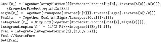
Figure 1.
Mathematica notebook to treat a VARMA model (6 lines!).
As mentioned in the conclusions of [26] (p. 12),
The open-source packages Octave and Maxima should be able to do the job since their symbolic integration procedure can work on matrices of functions, but they do not work presently. More developments would be needed to circumvent their failing integration.
- I tried with more recent versions without much success. Therefore, I had no other choice than to search for alternative approaches.
Meanwhile, it appeared that Mathematica version 13.3 has a new experimental procedure called ResidueSum for evaluating the integral of a rational function, based on Cauchy’s residue Theorem. The open-source symbolic computation software Maxima 5.47.0 offers a function called residue to evaluate a Cauchy residue provided that the poles within the unit circle are specified. The open-source scientific programming language Octave 8.1 is largely compatible with Mathworks Matlab and possesses a function residue but is numerical.
In several papers [8,9], we have used an algorithm [29] from Söderström in a numerical way. That algorithm is aimed at computing a circular integral of a rational function along the unit circle of the complex plane. That rational function has the form , where and are polynomials having their roots strictly inside and strictly outside, respectively, of the unit circle, and is a polynomial. The algorithm proceeds by using recurrences where the degrees of the polynomials are reduced one by one in turn until the integrand becomes a constant. Consequently, no integration is performed; computations are only performed on the coefficients of the polynomials.
3. Results
As a consequence of the arguments in Section 2, this article presents different solutions to compute the Fisher information matrix of ARMA and VARMA models for Mathematica, Maxima, and Octave. I first propose a symmetric alternative to the algorithm in [26] that is necessary for most of the approaches. Then, I use Cauchy’s residues for the three packages Mathematica, Maxima, and Octave. Finally, to circumvent the fact that Octave’s residue is numerical, I use a symbolic version of Söderström’s algorithm.
I illustrate the different methods in two examples.
Example 3.
I take the ARMA(2,2) model extracted from the ARMAX model used in [26] and first in [12]. It is based on the model defined by the equation , so and . I take . The model has parameters.
Example 4.
I take the VARMA(1,1) model treated by [33] extracted from the VARMAX model used in [18]. It is based on the model equation , with
I take . There are parameters.
3.1. An Alternative Integral Representation
The representation of the Fisher information matrix presented in (3)–(6) is nice but has the inconvenience of having polynomials in z and at several places. This is not convenient, neither for the use of Söderström’s algorithm in [29] nor for computing residues. Thus, I investigated an alternative integral representation of (6) that would be more symmetric in z and . Instead of integrating the matrix with and , I compute , the positive definite square root of , define , and exploit the identity
Hence, (6) can be equivalently obtained by
where is a block matrix with entries being rational functions in z while is a block matrix with entries being rational functions in . Moreover, by construction, the entries of have a denominator with roots outside the unit circle whereas those of are inside the unit circle. Consequently, we are able to compute Cauchy’s residues or to use that alternative representation for the algorithm of Söderström (1984) for a contour integral of a rational function.
To illustrate that alternative representation, let us consider a univariate model, so . Then, is an vector and is a vector. We perform a simplification of the rational functions and isolate the numerators and denominators. Then, the entry , of the product has as numerator and as denominator . Now, we can use either the residues at the roots of or Söderström’s algorithm with , , and .
3.2. Methods Using Cauchy’s Residues
It is well known that a contour integral of a meromorphic function can be evaluated as a sum of residues by using Cauchy’s residue theorem. We can use it to evaluate the integral in (6) or in (11). The sum includes only the residues that correspond to a pole inside the contour. Since version 13.3, Mathematica has a new experimental function ResidueSum for evaluating such an integral, based on Cauchy’s residue theorem.
A double loop over the rows and columns of the information matrix is needed because, presently, ResidueSum is unable to work on a matrix. The advantage is, however, that the double loop around ResidueSum can take care of the symmetry property of the information matrix, contrary to Integrate, as supposed (although I do not know the function’s internals). That double loop wis also necessary with the other packages. It appears that the code using ResidueSum is much faster than Integrate (see below). There is, however, a serious restriction on the size of the model, i.e., p, q, and r. For instance, , , and or , , and would work but not, in general, , , and or , , and because it would involve polynomials of degrees 5 or more for which there is no algebraic solution using radicals, by Abel–Ruffini theorem. This restriction is, of course, valid for the other packages using residues.
Both Octave and Maxima have a function residue to compute these residues. Maxima’s residue function is symbolic (provided that the poles can be computed symbolically). Note that the computation of these poles in Maxima should be carried out before calling the function, although this is not required by Mathematica. This implies using the solve function and managing the poles for their use in the call to residue.
Contrary to Maxima, Octave’s residue function is numerical, not symbolic. For Maxima and Octave, some care is needed in the case of multiplicity because only the terms corresponding to the first pole need to be used. This is performed for Octave in a function called residuesum.m, available in Supplementary Material S1.
3.3. An Algorithm for Integrating Rational Functions Around the Unit Circle
Ref. [29] is a working paper that describes an algorithm integrating rational functions around the unit circle. It is said that the algorithm is inspired by [34], whose aim was to evaluate an integral of a rational function along the whole imaginary axis. The working paper also contains an implementation: a Fortran function called CINT. In several papers [8,9], that algorithm was used in a numerical way. Here, I propose a symbolic variation programmed in Matlab/Octave.
Let , , and be polynomials with respective degrees , , and . We suppose the following:
- has all its zeros strictly inside the unit circle; and
- has all its zeros strictly outside the unit circle;
whereas there is no restriction on . We need to compute the contour integral
The algorithm has a finite number of steps with linearly transformed polynomials while keeping the integral’s value. At each step, one of the polynomials has a smaller degree, i.e., with decreasing , , and . At the end, or , and the calculation is elementary.
Since the symbolic Matlab/Octave program and its procedures are too long to be included in these pages, they are available as Supplementary Materials. This is carried out for Octave in a function called circintrat.m, available as Supplementary Material S2. Note that the original numerical Fortran code is still there but presented as comments.
3.4. A New Algorithm for Mathematica
In [26], we used the symbolic integration in (6) not as a circular integral but after a change of variable , i.e., using a definite trigonometric integral over . We showed a figure with the most important part of the Mathematica notebook. Figure 2, part (a), shows the part of the notebook using my alternative representation of Section 3.1 with the computation of the contour integral directly, without a change of variable.
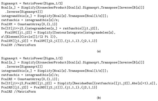
Figure 2.
Parts of a Mathematica notebook showing two new procedures for computing the AFIM. (a) Computation of the contour integral using the alternative representation of Section 3.1. (b) Computation using ResidueSum, as in Section 3.2.
Moreover, the new ResidueSum function of Mathematica version 13.3 for evaluating the integral of a rational function, based on Cauchy’s residue theorem, is also added in Figure 2, part (b). The whole notebooks are available as Supplementary Materials S3 and S4 for Examples 3 and 4, respectively, with their output in Supplementary Materials S5 and S6, respectively. There was no reason to adapt the algorithm in [29] to Mathematica since we already have several computationally efficient solutions.
Let us now consider the application in the two examples.
Example 5. 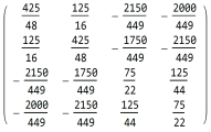 or
or 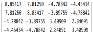
For the univariate ARMA(2,2) model with four parameters, with each of the three methods, the one in [26], the variant in Section 3.1, or the experimental ResidueSum function, we have the same results:
or The determinant of the exact AFIM is given by the fraction . The model is therefore identifiable.
Example 6.
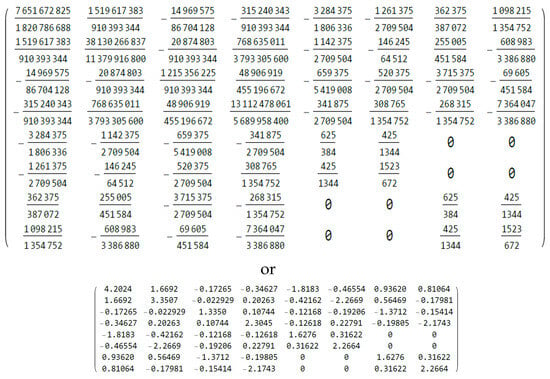
For the VARMA(1,1) model with eight parameters, using either of the three methods, we obtain the same matrix of rational numbers shown in Figure 3. The matrix of numerical values is also shown. The smallest eigenvalue of the exact AFIM is ; hence, the model is identifiable. Note that, like in [26] (Example 1 and Figure 5), it would be possible to have a very small number of symbolic parameters (such as a or b) instead of fractions (like ) for the coefficients, but the resulting output would be expressions using these literal parameters.
Figure 3.
AFIM for Example 6 in exact rational and numerical forms, as output from Mathematica 14.0.
3.5. An Algorithm for Maxima
As explained in Section 2, although Maxima is, in principle, able to symbolically evaluate an integral of a matrix, it failed to provide the correct results. Hopefully, I found a residue function, but it is essential to describe the condition on the roots. The function does not work on a matrix, so we have to perform a double loop on the rows and columns (taking into account the symmetry of the matrix, of course) and symbolically evaluate the polynomials involved in each entry at the numerator and at the denominator. That required using the alternative integral representation in Section 3.1 because the asymmetric original representation used in [26] makes it difficult to separate the roots with respect to the unit circle. For the two examples, the results obtained with Maxima are exactly the same as with Mathematica. I have used wxMaxima 23.05.1. I discuss the practical aspects and the timings of the examples in Section 4. The whole Maxima workspaces are available as Supplementary Materials S7 and S8 for Examples 3 and 4, respectively, with their output in Supplementary Materials S9 and S10, respectively.
3.6. An Algorithm for Octave
Octave is a scientific programming language that is largely compatible with Matlab but it is open-source. Like Matlab, it contains a symbolic computation toolbox. It is based on Python SymPy. As for Maxima, Octave is, in principle, able to symbolically evaluate an integral of a matrix but it failed to provide the correct results.
Like Maxima, there is also a residue function but it is numerical, not symbolic, and, hence, unable to provide the same exact results as Mathematica and Maxima. To have an exact expression for the Fisher information matrix, I considered Söderström’s algorithm (1984) described in Section 3.3 and ported to the Matlab/Octave language. As for Maxima, it is not possible to implement either residuesum.m or circintrat.m straightforwardly on matrices: we have to perform a double or a triple loop on the rows and the columns and a summation index in order to prepare the polynomials to be used. Here, the alternative integral representation of Section 3.1 is again essential. The whole scripts are available as Supplementary Materials S11 and S12 for Examples 3 and 4, respectively, with their output in Supplementary Materials S13 and S14, respectively.
In the two examples, the results are the same as for Mathematica, under the form of fractions for circintrat.m or decimal numbers for residuesum.m. I have used Octave 8.1. Note that there is a pending problem for treating the examples in version 9.2. I again discuss the practical aspects and the timings in Section 4.
3.7. Application on Examples 3 and 4
The difference between Mathematica, Maxima, and Octave is in the computation time of the different methods. This is discussed in Section 4.
4. Discussion
In Section 3.4, Section 3.5 and Section 3.6, I have proposed algorithms for the computation of the Fisher information matrix of univariate ARMA or multivariate VARMA time-series models.
These algorithms are all based on the new integral representation in Section 3.1 and one of them makes use of Söderström’s algorithm in [29] described in Section 3.3.
I have used the following in Mathematica:
- The method proposed in [26];
- The variant proposed in Section 3.3;
- The method based on the experimental ResidueSum.
- We have seen in Section 3.3 that the three methods give the same exact results.
I have used in Maxima the method based on residue, which has the disadvantage of requiring the preliminary determination of the poles of the rational functions being involved. I could have considered porting circintrat.m to Maxima but this would require programming in LISP.
In the case of Octave, I have used the following two methods:
- The symbolic method using circintrat.m based on Söderström’s algorithm that gives the same exact results as Mathematica;
- The numerical method based on a function residuesum.m that gives approximately the same numerical results, at least in the examples.
- There is no doubt that the latter method with the function residuesum.m in Octave can lead to problems in near-singular cases.
The computation time of the different methods in Mathematica, Maxima, and Octave is quite variable. I give some orders of magnitude for the different methods and packages in Table 1 for Example 3 and Table 2 for Example 4. They are given in seconds but, of course, they depend on the processor (an x64-based processor 11th Gen Intel Core i7-1165G7 clocked at 2.80 GHz, with 16 GB of installed RAM, and under Windows 11 version 23H2) and the charge. I took averages over 10,000 runs for the Maxima fast Example 3, 100 runs for Mathematica trigonometric integrals and the two slow methods with Octave, and 1000 runs for all the other methods. For Mathematica, I had to slightly change the model for each repetition because, otherwise, the results after the first run would be taken from the internal cache. For Example 3, the clear winner is residue in Maxima. For Example 4, the method of [26] in Mathematica was the best one, followed by residue in Maxima. Among the two methods used with Octave, the exact method using circintrat.m takes only about twice the time as the approximate method based on residuesum.m. They are much slower than the other methods. For Maxima, the reservations discussed previously about the need to determine the poles make it uneasy. Moreover, even for slightly more complex models, the impossibility of obtaining the poles symbolically will not allow us to use the methods based on Cauchy’s residues exactly, including ResidueSum in Mathematica. An alternative that is currently slow in Octave but does not require solving polynomial equations is provided by Söderström’s algorithm in [29].

Table 1.
Computation time for running Example 3.
Table 2.
Computation time for running Example 4.
5. Conclusions
To summarize, I have shown that a slight change in the presentation of the integrand (by making it more symmetric) in the integration procedure in the Wolfram Mathematica notebook proposed by [26] has allowed the development of two new methods and to address two other software packages, GNU Maxima and GNU Octave. Using Cauchy residues can lead to an improvement and is the solution for GNU Maxima, where the integration procedure does not work well presently. I have also tried a second open-source program with GNU Octave, where integration fails and the residue function is numeric. I have nevertheless obtained the correct results with a symbolic implementation of Söderström’s algorithm [29], although it is much slower than with the other solutions. I have mentioned in Section 4 the limitations of the methods based on residues.
As I have said in Section 2, there would be no problem for handling linearly and possibly lagged explanatory or exogenous variables, e.g., ARMAX or VARMAX models, since that would add a second matrix integral for which the methods discussed in this paper can be used. Consequently, there are now several exact procedures to check the identifiability of the ARMA, ARMAX, VARMA, and VARMAX models.
On the contrary, working with multiplicative seasonal ARMA or VARMA models, like in [10,11], is not so immediate but should be possible.
A reviewer has questioned the need for normality and why I did not consider the R language.
I have made clear that normality is related to the likelihood function. This means that the exact AFIM is obtained if parameter estimation is performed by maximizing the Gaussian quasi-likelihood or by least-squares, whatever the true distribution of the model errors.
If we know the distribution of , another likelihood can be considered that should provide another AFIM, but there are relatively few popular alternatives except for count time series, e.g., [35,36,37,38,39], with a few exceptions like [40] or [41]. When we use the Gaussian likelihood instead of the appropriate likelihood, the information matrix is multiplied by a known factor, under very general conditions. As mentioned by [42] or [43], that factor is equal to for the logistic distribution or 2 for the Laplace distribution. This means that it is possible, in the latter case and with the correct likelihood, to decrease the asymptotic standard errors of the parameter estimators by a factor of ; see also [16].
Alternatively, it is possible to use adaptive estimation methods like in [42] or R-estimation methods that are based on ranks. R-estimation is relatively easy for univariate time series like in [44] but much more difficult in the multivariate case, e.g., [45] or [46] and the references cited therein.
As for the R language, it is true that I did not consider R as a computer algebra system (CAS). After a search, I found at least two R packages on CRAN that offer exact computation and would be worth being considered: Caracas and Ryacas, which can be used for symbolic computations within R. Caracas offers an interface to SymPy, whereas Ryacas offers an interface to Yacas. Time constraints did not allow me to add them to the present study but I intend to consider them in the future. An alternative would be to use Python directly with SymPy. SymPy and Yacas offer matrices, polynomials, and integration, although not contour integration, apparently. I doubt that the program will be as short as the Mathematica code in Figure 1 and Figure 2. There is no reason why the Söderström approach would not work after reprogramming in the R language.
Supplementary Materials
The following supporting information can be downloaded at: https://www.mdpi.com/article/10.3390/info16010016/s1. S1, Type: Octave function residuesum (.m)—for use in S11 and S12; S2, Type: Octave function circintrat (.m)—for use in S11 and S12; S3, Type: Mathematica notebook (.nb)—input for Example 3 in Mathematica; S4, Type: Mathematica notebook (.nb)—input for Example 4 in Mathematica; S5, Type: Mathematica notebook (.pdf)—output of Example 3 from Mathematica; S6, Type: Mathematica notebook (.pdf)—output of Example 4 from Mathematica; S7, Type: Maxima workspace (.wxmx)—input for Example 3 in Maxima; S8, Type: Maxima workspace (.wxmx)—input for Example 4 in Maxima; S9, Type: Maxima workspace (.pdf)—output of Example 3 from Maxima; S10, Type: Maxima workspace (.pdf)—output of Example 4 from Maxima; S11, Type: Octave script (.m)—input for Example 3 in Octave; S12, Type: Octave script (.m)—input for Example 4 in Octave; S13, Type: Octave output (.pdf)—output of Example 3 from Octave; S14, Type: Octave output (.pdf)—output of Example 4 from Octave.
Funding
This research received no external funding.
Institutional Review Board Statement
Not applicable.
Informed Consent Statement
Not applicable.
Data Availability Statement
No data were used.
Acknowledgments
I acknowledge moral support from my research department ECARES and my university. I thank my longtime coauthor André Klein not only for his encouragement but also for his comments on the preceding versions of this project.
Conflicts of Interest
The author declares no conflicts of interest.
Abbreviations
The following abbreviations are used in this manuscript:
| AFIM | Asymptotic Fisher information matrix |
| AR | Autoregressive |
| ARMA | Autoregressive moving average |
| ARMAX | Autoregressive moving average with explanatory variables |
| MA | Moving average |
| SISO | Single-input single-output |
| VARMA | Vector autoregressive moving average |
| VARMAX | Vector autoregressive moving average with explanatory variables |
References
- Hannan, E.J. The identification of vector mixed autoregressive-moving average systems. Biometrika 1969, 56, 223–225. [Google Scholar]
- Hannan, E.J. The identification problem for multiple equation systems with moving average errors. Econometrica 1971, 39, 751–765. [Google Scholar] [CrossRef]
- Hannan, E.J.; Deistler, M. The Statistical Theory of Linear Systems; Wiley: New York, NY, USA, 1988. [Google Scholar]
- Whittle, P. Estimation and information in time series. Ark. Mat. 1953, 2, 423–434. [Google Scholar] [CrossRef]
- Box, G.E.P.; Jenkins, G.M.; Reinsel, G.C.; Ljung, G.M. Time Series Analysis Forecasting and Control, 5th ed.; Wiley: Hoboken, NJ, USA, 2015. [Google Scholar]
- Godolphin, E.J.; Unwin, J.M. Evaluation of the covariance matrix for the maximum likelihood estimator of a Gaussian autoregressive-moving average process. Biometrika 1983, 70, 279–284. [Google Scholar] [CrossRef]
- Porat, B.; Friedlander, B. Computation of the exact information matrix of Gaussian time series with stationary random components. IEEE T. Acoust. Speech 1986, 14, 118–130. [Google Scholar] [CrossRef]
- Klein, A.; Mélard, G. On algorithms for computing the covariance matrix of estimates in autoregressive-moving average models. Comput. Stat. Q. 1989, 5, 1–9. [Google Scholar]
- Klein, A.; Mélard, G. Fisher’s information matrix for seasonal autoregressive-moving average models. J. Time Ser. Anal. 1990, 11, 231–237. [Google Scholar] [CrossRef]
- Godolphin, E.J.; Bane, S.R. On the evaluation of the information matrix for multiplicative seasonal time-series models. J. Time Ser. Anal. 2005, 27, 167–190. [Google Scholar] [CrossRef]
- Godolphin, E.J.; Godolphin, J.D. A note on the information matrix for multiplicative seasonal autoregressive moving average models. J. Time Ser. Anal. 2007, 28, 167–190. [Google Scholar] [CrossRef]
- Gevers, M.; Ljung, L. Optimal experiment designs with respect to the intended model application. Automatica 1986, 22, 543–544. [Google Scholar] [CrossRef]
- Klein, A.; Spreij, P. On Fisher’s information matrix of an ARMAX process and Sylvester’s resultant matrices. Linear Algebra Appl. 1996, 237/238, 579–590. [Google Scholar] [CrossRef]
- Ljung, L.; Söderström, T. Theory and Practice of Recursive Identification; MIT Press: Cambridge, MA, USA, 1983. [Google Scholar]
- Young, P.C. Recursive Estimation and Time-Series Analysis: An Introduction for the Student and the Practitioner, 4th ed.; Springer: Heidelberg, Germany, 2011. [Google Scholar]
- Klein, A.; Mélard, G. An algorithm for computing the asymptotic Fisher information matrix for seasonal SISO models. J. Time Ser. Anal. 2004, 25, 627–648. [Google Scholar] [CrossRef]
- Newton, H.J. The information matrices of the parameters of multiple mixed time series. J. Multivar. Anal. 1978, 8, 317–323. [Google Scholar] [CrossRef]
- Klein, A.; Mélard, G.; Spreij, P. On the resultant property of the Fisher information matrix of a vector ARMA process. Linear Algebra Appl. 2005, 403, 291–313. [Google Scholar] [CrossRef]
- Athanasopoulos, G.; Vahid, F. VARMA versus VAR for macroeconomic forecasting. J. Bus. Econ. Stat. 2008, 26, 237–252. [Google Scholar] [CrossRef]
- Bao, Y.; Hua, Y. On the Fisher information matrix of a vector ARMA process. Econ. Lett. 2014, 123, 14–16. [Google Scholar] [CrossRef]
- Zadrozny, P.A. Analytical derivatives for estimation of linear dynamic models. Comput. Math. Appl. 1989, 18, 539–553. [Google Scholar] [CrossRef]
- Lomba, J.T. Estimation of Dynamic Econometric Models with Errors in Variables; Springer: Berlin, Germany, 1990. [Google Scholar]
- Zadrozny, P.A. Errata to ’Analytical derivatives for estimation of linear dynamic models’. Comput. Math. Appl. 1992, 24, 289–290. [Google Scholar] [CrossRef]
- Mittnik, S.; Zadrozny, P.A. Asymptotic distributions of impulse responses, step responses, and variance decompositions of estimated linear dynamic model. Econom. 1993, 61, 857–870. [Google Scholar] [CrossRef]
- Jerez, M.; Casals, J.; Sotoca, S. Signal Extraction for Linear State-Space Models; Lambert Academic Publishing: Saarbrücken, Germany, 2011. [Google Scholar]
- Klein, A.; Mélard, G. An algorithm for the Fisher information matrix of a VARMAX process. Algorithms 2023, 16, 364. [Google Scholar] [CrossRef]
- Klein, A.; Spreij, P. Tensor Sylvester matrices and the Fisher information matrix of VARMAX processes. Linear Algebra Appl. 2010, 432, 1975–1989. [Google Scholar] [CrossRef]
- Dym, H. Linear Algebra in Action, 2nd ed.; American Mathematical Society: Providence, RI, USA, 2013. [Google Scholar]
- Söderström, T. Description of a Program for Integrating Rational Functions Around the Unit Circle; Technical Report 8467R; Department of Technology, Uppsala University: Uppsala, Sweden, 1984; Unpublished work. [Google Scholar]
- Düker, M.-C.; Matteson, D.S.; Tsay, R.S.; Wilms, I. Vector autoregressive moving average models: A review. arXiv 2024, arXiv:2406.19702. [Google Scholar]
- Gourieroux, C.; Monfort, A.; Trognon, A. Pseudo maximum likelihood methods: Theory. Econometrica 1984, 52, 681–700. [Google Scholar] [CrossRef]
- Klein, A.; Spreij, P. Matrix differential calculus applied to multiple stationary time series and an extended Whittle formula for information matrices. Linear Algebra Appl. 2010, 430, 674–691. [Google Scholar] [CrossRef]
- Mélard, G. An indirect proof for the asymptotic properties of VARMA model estimators. Econom. Stat. 2022, 21, 96–111. [Google Scholar] [CrossRef]
- Peterka, V.; Vidinčev, P. Rational-fraction approximation of transfer functions. In Proceedings of the IFAC Symposium on Identification in Automatic Control Systems, Prague, Czechoslovakia, 12–17 June 1967. [Google Scholar]
- Davis, R.A.; Dunsmuir, W.T.M.; Streett, S.B. Maximum likelihood estimation for an observation driven model for Poisson counts. Methodol. Comput. Appl. 2005, 7, 149–159. [Google Scholar] [CrossRef]
- Fokianos, K.; Rahbek, A.; Tjøstheim, D. Poisson autoregression. J. Am. Stat. Assoc. 2009, 104, 1430–1439. [Google Scholar] [CrossRef]
- Fokianos, K. Count time series models. In Time Series: Methods and Applications, Handbook of Time Series Analysis; Subba Rao, T., Subba Rao, S., Rao, C.R., Eds.; Elsevier: Amsterdam, The Netherlands, 2012; Volume 30, pp. 315–347. [Google Scholar]
- Liboschik, T.; Fokianos, K.; Fried, R. tscount: An R package for analysis of count time series following generalized linear models. J. Stat. Softw. 2017, 82, 5. [Google Scholar] [CrossRef]
- Fokianos, K.; Støve, B.; Tjøstheim, D.; Doukhan, P. Multivariate count autoregression. Bernoulli 2020, 26, 471–499. [Google Scholar] [CrossRef]
- Benjamin, M.A.; Rigby, R.A.; Stasinopoulos, M.D. Fitting non-Gaussian time series models. In COMPSTAT 1998: Proceedings in Computational Statistics; Payne, R., Green, P., Eds.; Physica Verlag: Heidelberg, Germany, 1998; pp. 191–196. [Google Scholar]
- Kugiumtzis, D.; Bora-Senta, E. Gaussian analysis of non-Gaussian time series. Bruss. Econ. Rev. 2010, 53, 295–322. [Google Scholar]
- Drost, F.C.; Klaassen, C.A.J.; Werker, B.J.M. Adaptive estimation in time-series models. Ann. Stat. 1997, 25, 786–818. [Google Scholar] [CrossRef]
- Hallin, M.; Werker, B.J.M. Optimal testing for semiparametric AR models: From Lagrange multipliers to autoregression rank scores and adaptive tests. In Asymptotics, Nonparametrics and Time Series; Ghosh, S., Ed.; Marcel Dekker: New York, NY, USA, 1999; pp. 295–350. [Google Scholar]
- Hallin, M.; Paindaveine, D. Rank-based optimal tests of the adequacy of an elliptic VARMA model. Ann. Stat. 2004, 32, 2642–2678. [Google Scholar] [CrossRef]
- Hallin, M.; La Vecchia, D. R-estimation in semiparametric dynamic location-scale models. J. Econom. 2017, 196, 233–247. [Google Scholar] [CrossRef]
- Hallin, M.; La Vecchia, D.; Liu, H. Center-outward R-estimation for semiparametric VARMA models. J. Am. Stat. Assoc. 2020, 117, 925–938. [Google Scholar] [CrossRef]
Disclaimer/Publisher’s Note: The statements, opinions and data contained in all publications are solely those of the individual author(s) and contributor(s) and not of MDPI and/or the editor(s). MDPI and/or the editor(s) disclaim responsibility for any injury to people or property resulting from any ideas, methods, instructions or products referred to in the content. |
© 2024 by the author. Licensee MDPI, Basel, Switzerland. This article is an open access article distributed under the terms and conditions of the Creative Commons Attribution (CC BY) license (https://creativecommons.org/licenses/by/4.0/).