Quantum Algorithms for the Multiplication of Circulant Matrices and Vectors

Abstract

This article presents two quantum algorithms for computing the product of a circulant matrix and a vector. The arithmetic complexity of the first algorithm is $O(N{log}^{2}N)$ in most cases. For the second algorithm, when the entries in the circulant matrix and the vector take values in $\mathbb{C}$ or $\mathbb{R}$, the complexity is $O(\sqrt{N}{log}^{2}N)$ in most cases. However, when these entries take values from positive real numbers, the complexity is reduced to $O({log}^{3}N)$ in most cases, which presents an exponential speedup compared to the classical complexity of $O(NlogN)$ for computing the product of a circulant matrix and vector. We apply this algorithm to the convolution calculation in quantum convolutional neural networks, which effectively accelerates the computation of convolutions. Additionally, we present a concrete quantum circuit structure for quantum convolutional neural networks.

1. Introduction

Quantum computing, as a disruptive technology, has received widespread attention from various fields, since it can efficiently accelerate the solving of some fundamental computational problems. For example, Shor’s algorithm [1] can solve the factorization problem in polynomial time, posing a great threat to modern cryptography in theory. Grover’s algorithm [2] can achieve a square-root speedup in unstructured search. The HHL algorithm [3] proposed in 2006 has an exponential speedup in solving linear equations.

As a linear equation solver, the HHL algorithm consists of three main parts. The first part employs quantum phase estimation to achieve the eigenvalues of the matrix being calculated. The second part applies quantum controlled gates to flip the auxiliary qubits based on the given eigenvalues. The third part uses the inverse of quantum phase estimation to undo the entanglement and restore some of the auxiliary qubits. By measuring the remaining auxiliary qubits, one can obtain the target state. By modifying the second step of the HHL algorithm, we can easily apply the idea of the HHL algorithm to matrix–vector multiplication. It should be noted that the complexity of the HHL algorithm depends not only on the size of the matrix but also on the condition number of the matrix. The condition number of a matrix is an indicator of the sensitivity of the matrix to changes in the result, and is an inherent property of the matrix. Therefore, it is difficult to manually constrain the condition number of the matrix. There are some types of matrices that may have a high condition number but contain some specific structures, which could lead to more efficient computation. Circulant matrices are one of these types and, in this paper, we focus on their computation.

Circulant matrices have been well studied in both classical and quantum settings. In the classical setting, it was shown that the product of a circulant matrix and a vector of size N can be computed with $O(NlogN)$ operations using FFT (Fast Fourier Transformation) [4]. By expressing a Toeplitz matrix as a circulant matrix, Golub and van Loan showed that a Toeplitz matrix and a vector can also be multiplied in time $O(NlogN)$ [4]. Circulant matrices and related structured matrices were also studied in [5,6,7]. In the quantum setting, different quantum expressions for the circulant matrix were presented in [8,9,10]. Reference [8] presents a quantum construction method for cyclic matrices. Where the Toeplitz matrix can serve as a submatrix of the cyclic matrix, reference [9] provides an asymptotic method for solving Toeplitz systems. Reference [10] applies cyclic matrices to quantum string processing.

In this paper, we propose two new quantum algorithms for circulant matrix–vector multiplication, which take advantage of the features of quantum mechanics and have better computational complexity compared to classical algorithms. For the first algorithm we propose, the complexity is $O(N{log}^{2}N)$ in most case. For the second algorithm, if the elements in the circulant matrix and vector are randomly chosen from $\mathbb{R}$ or $\mathbb{C}$ with a norm no larger than d, then the proportion of matrices and vectors that can be computed with complexity $O(\sqrt{N}{log}^{2}N)$ approaches 1 as the dimension of the matrix increases. Similarly, if the elements are randomly chosen from ${\mathbb{R}}^{+}$ with a norm no larger than d, then the proportion of matrices that can be computed with complexity $O({log}^{3}N)$ also approaches 1 as the dimension increases.

Theorem 1. 

There exists two quantum algorithms which compute the multiplication of the circulant matrix and vector. For the first algorithm, it computes the multiplication of a circulant matrix and a vector over $\mathbb{C}$ (or $\mathbb{R})$ with a probability of at least $1-{\displaystyle \frac{1}{N}}$ and complexity $O(N{log}^{2}N)$, where N is the dimension of the matrix, and the proportion of the circulant matrix and vector combinations that can be effectively computed approaches 1 as the dimension increases. For the second algorithm, it computes the multiplication of the most circulant matrix and vector over $\mathbb{C}$ (or $\mathbb{R})$ with a probability of at least $1-{\displaystyle \frac{1}{N}}$ and complexity $O(\sqrt{N}{log}^{2}N)$, where N is the dimension of the matrix, and the proportion of the circulant matrix and vector combinations that can be effectively computed approaches 1 as the dimension increases.

Compared to the approach similar to the HHL algorithm, our second algorithm has two advantages. Firstly, our second algorithm directly performs calculations on quantum states without the need for Hamiltonian simulations, thus reducing computational complexity and errors. Secondly, our second algorithm does not have the process of quantum phase estimation (QPE), thus reducing the use of auxiliary bits and errors. Our second algorithm also has a measurement step and has the same complexity as the HHL approach during measurement. The comparison is shown in the Table 1. In particular, when the circulant matrix and vector values are in ${\mathbb{R}}^{+}$, the algorithm complexity is logarithmic with respect to the size of the matrix.

Table 1. Comparison of HHL method, Algorithm 1, and Algorithm 2.

	HHL Method	Algorithm 1	Algorithm 2
Hamiltonian simulation	need	need not	need not
QPE	need	need not	need not
Number of auxiliary qubits	$O(log(N))$	$2log(N)+2$	$log(N)$
Measurement probability	$O(\sqrt{N})$	$O(N)$	$O(\sqrt{N})$
Error	exist	no	no

Furthermore, we apply our algorithms in convolution computation, which is an important and fundamental problem in quantum machine learning (QML). The field of quantum machine learning has been developing rapidly in recent years. Machine learning algorithms suffer from computational bottlenecks as the dimensionality increases. To promote experimental progress towards realizing quantum information processors, the approach of using quantum computers to enhance conventional machine learning tasks was proposed, and this led to the development of quantum convolutional neural networks (QCNNs). The earliest QCNN was proposed in [11] for solving quantum many-body problems. Subsequently, in [12,13], QCNNs for image recognition were discussed. The difference of their results is that the quantum circuit in [12] is a purely random quantum circuit, while the quantum circuit in [13] has a simple design. In [12], the authors presented real experiments to confirm that their algorithm still has some effect even when using a fully random quantum circuit. The quantum circuit designed in [13] only entangles different qubits without a more specific definition of the quantum circuit. In this paper, we present an effective quantum circuit for computing convolutions, which may be used as a sub-circuit in the quantum circuit of QCNNs.

The structure of this article is as follows. In Section 2, we introduce circulant matrices and some basics of quantum computing, and present some quantum circuit structures that will be used in the quantum algorithms for circulant matrix–vector multiplication. In Section 3, we describe the details of our new algorithms and analyze their running times. As both algorithms involve quantum measurements, Section 4 presents a probability analysis of the measurements and, for parts where theoretical analysis is not available, we present experimental results to support our algorithms. In Section 5, we discuss the specific application of circulant matrix–vector multiplication in convolution computation. Finally, conclusions and future directions are presented in Section 6.

2. Preliminaries

In this section, we will present some background information that will be used in our later discussion of the circulant matrix–vector algorithm. This includes properties of circulant matrices, existing results in quantum computing, and structures of quantum circuits, as well as the effects that these structures can achieve in quantum circuits.

2.1. Circulant Matrix

For any vector $\mathbf{a}$$={(a_0,a_1,\dots ,a_{N-1})}^{\top }$ in ${\mathbb{C}}^N$, its corresponding circulant matrix is denoted by $\mathbf{A}$ and is represented as follows:

$$\mathbf{A}=\left(\begin{array}{ccccc}{a}_0& a_1& a_2& \dots & a_{N-1}\\ a_{N-1}& a_0& a_1& \dots & a_{N-2}\\ ⋮& ⋮& ⋮& \ddots & ⋮\\ a_1& a_2& a_3& \dots & a_0\end{array}\right)$$

(1)

The circulant matrix $\mathbf{A}$ can be represented as a linear combination of matrix $\mathbf{T}$, denoted as

$$\begin{array}{c}\hfill \mathbf{A}=\sum _{j=0}^{N-1}{a}_j{\mathbf{T}}^j,\end{array}$$

(2)

where $\mathbf{T}$ is the cyclic permutation matrix and can be represented as

$$\mathbf{T}={\left(\begin{array}{ccccc}0& 1& 0& \dots & 0\\ 0& 0& \ddots & \ddots & ⋮\\ ⋮& ⋮& \ddots & \ddots & 0\\ 0& 0& \dots & 0& 1\\ 1& 0& \dots & 0& 0\end{array}\right)}_{N\times N}$$

(3)

In addition, a circulant matrix can also be diagonalized by a Fourier matrix of the same order. Let $\mathbf{F}$ be the Fourier matrix in ${\mathbb{C}}^{N\times N}$, and let $\omega =e^{{\displaystyle \frac{2\pi i}{N}}}$; then, $\mathbf{F}$ can be expressed as

$$\mathbf{F}=\left(\begin{array}{ccccc}1& 1& 1& \dots & 1\\ 1& \omega & {\omega }^2& \dots & {\omega }^{N-1}\\ ⋮& ⋮& ⋮& \ddots & ⋮\\ 1& {\omega }^{N-1}& {\omega }^{2(N-1)}& \dots & {\omega }^{{(N-1)}^2}\end{array}\right)$$

(4)

Using $\mathbf{F}$, we can diagonalize $\mathbf{A}$ to a diagonal matrix ${\mathbf{A}}^{\prime }$. Specifically, if we denote $diag\left\{{\mathbf{F}}^{-\mathbf{1}}\mathbf{a}\right\}$ as the diagonal matrix with ${\mathbf{F}}^{-\mathbf{1}}\mathbf{a}$ on its diagonal, then, we have

$$\begin{array}{c}\hfill {\mathbf{A}}^{\prime }={\displaystyle \frac{1}{N}}{\mathbf{FAF}}^{-1}=diag\left\{{\mathbf{F}}^{-1}\mathbf{a}\right\}.\end{array}$$

(5)

In this paper, we are calculating the matrix–vector multiplication of a circulant matrix $\mathbf{A}$ and a vector $\mathbf{x}={(x_0,x_1,\dots ,x_{N-1})}^{\top }$ over $\mathbb{C}$. Here, $\mathbf{A}$ is given by a vector $\mathbf{a}={(a_0,a_1,\dots ,a_{N-1})}^{\top }$, and their correspondence can be found in Equation (1). It is easy to check that the k-th eigenvalue of $\mathbf{A}$ is ${\lambda }_k={\sum }_{j=0}^{N-1}{a}_j{\omega }^{-jk}$, and ${\Lambda }_k={\displaystyle \frac{1}{\sqrt{N}}}{(1,{\omega }^{-k},\dots ,{\omega }^{-k(N-1)})}^{\top }$ is the corresponding eigenvector. Moreover, we have $\mathbf{x}={\sum }_{k=0}^{N-1}({\displaystyle \frac{1}{\sqrt{N}}}{\sum }_{j=0}^{N-1}{x}_j{\omega }^{jk}){\Lambda }_k$ and, in the following, we denote ${\displaystyle \frac{1}{\sqrt{N}}}{\sum }_{j=0}^{N-1}{x}_j{\omega }^{jk}$ by ${\lambda }_k^x$ for simplicity.

To compute matrix–vector multiplication by a quantum algorithm, we need to represent the given two vectors by quantum states. The modulus squared of the coefficients of the quantum state corresponds to the probability of measuring that quantum state. Therefore, we first normalize the two given vectors and then convert them into the representation of quantum states. Unless otherwise specified, the vectors $\mathbf{a}$ and $\mathbf{x}$ we use later are both in the normalized form. As argued in most of quantum algorithms, we always assume that the quantum states $|a⟩={\sum }_{j=0}^{N-1}{a}_j|j⟩$ and $|x⟩={\sum }_{j=0}^{N-1}{x}_j|j⟩$ are already effectively prepared and we can directly use them for calculation. For example, our algorithm can serve as a subroutine in a larger algorithm and, in this case, the required quantum states $|a⟩$ and $|x⟩$ have already been generated. Generally speaking, it is difficult to prepare an arbitrary initial state, and there are only a few methods available now [14,15,16].

2.2. Quantum Computing

Definition 1. 

Let $n\ge 0$ be an integer, and $N=2^n$. The quantum Fourier transform on n qubits is defined by

$$\begin{array}{c}\hfill F_N:|x⟩\to {\displaystyle \frac{1}{\sqrt{2^n}}}\sum _{y=0}^{2^n-1}{e}^{2\pi ixy/2^n}|y⟩(0\le x\le 2^n-1)\end{array}$$

(6)

The complexity of the quantum Fourier transform is $O(n^2)$, and its quantum circuit diagram is as shown in Figure 1.

Figure 1. Quantum circuit for the quantum Fourier transform.

Next, we introduce the quantum amplitude amplification algorithm [17]. The quantum amplitude amplification algorithm can be classified into two types: the first type is when we already know the success rate of the target algorithm, while the second type is when we only know the possible values of the target algorithm. Both types achieve quadratic speedup. The algorithm can be described as follows.

There exists a quantum algorithm QSearch with the following property. Let $\mathcal{A}$ be any quantum algorithm that uses no measurements, and let $\chi :\mathbb{Z}\to \{0,1\}$ be any Boolean function. The Boolean function $\chi :\mathbb{Z}\to \{0,1\}$ induces a partition of the values of algorithm $\mathcal{A}$ into a direct sum of two subspaces, a good subspace and a bad subspace. The probability that the measurement result of the quantum algorithm $\mathcal{A}$ falls onto a good subspace is a. Algorithm QSearch finds a good solution using an expected number of applications of $\mathcal{A}$ and ${\mathcal{A}}^{-1}$, which are in $O({\displaystyle \frac{1}{\sqrt{a}}})$ if $a>0$, and otherwise runs forever. Please refer to [17] for more specific details.

2.3. Quantum Circuit

Here, we will introduce some quantum circuits that we will use and their roles.

Quantum Arithmetic Operation

We only need addition among quantum arithmetic operations. Here, we use the quantum adder given in [18], which consists of two parts. The first part is the calculation of carry, composed of the sub-circuit $\mathbf{MAJ}$, and the second part is the addition process using the carry calculation, composed of the sub-circuit $\mathbf{UMA}$. This adder is an in-place circuit, and its result is stored in the second register to reduce the number of qubits used. The relevant structures and circuit diagrams of the sub-circuits are shown below (calculate $a_2{a}_1{a}_0+b_2{b}_1{b}_0=c_3{s}_2{s}_1{s}_0$).

In Figure 2, M and U correspond to the sub-circuits $\mathbf{MAJ}$ and $\mathbf{UMA}$ in Figure 3, respectively, as detailed below:

Figure 2. Quantum addition circuit.

Figure 3. Sub-circuits of quantum addition circuit.

From the above circuit diagrams, we can see that the number of gates required to perform the addition of two n-bit numbers is $O(n)$.

2.4. Quantum Circuit for the ${\mathit{U}}^{\mathit{i}}$ Transformation

In this subsection, we suppose that we have the quantum circuit for the unitary matrix U; then, we introduce the quantum circuit for the $U^i$ transformation, which appears as a sub-circuit in quantum phase estimation. Specifically, given a quantum state $|a⟩$ and a unitary matrix U, the $U^j$ transformation

$${|0⟩}^{\otimes n}|a⟩\to \sum _{i=0}^{2^n-1}{\displaystyle \frac{1}{\sqrt{2^n}}}|i⟩U^i|a⟩$$

(7)

can be implemented as shown in Figure 4.

Figure 4. Quantum controlled-U circuit.

This circuit requires n controlled-U gates and performs a total of $O(n)$ quantum gates. Later, we will present the specific structure of the U gate to analyze the complexity of our first algorithm.

2.4.1. Quantum Circuit for the Cyclic Permutation

According to Equation (2) in Section 2.1, we know that the circulant matrix $\mathbf{A}$ can be represented by the cyclic permutation matrix $\mathbf{T}$. Here, we present a specific implementation for $\mathbf{T}$, where $\mathbf{T}$ is a $2^n\times 2^n$ cyclic permutation matrix.

Let $\mathbf{F}$ be the $2^n\times 2^n$ Fourier matrix. It is easy to check that

$${\mathbf{T}}^{\prime }={\mathbf{FTF}}^{-\mathbf{1}}=diag\{{\omega }^0,{\omega }^{-1},\dots ,{\omega }^{-(2^n-1)}\}$$

(8)

is a diagonal unitary matrix, and ${\mathbf{T}}^{\prime }$ can be implemented in Figure 5:

Figure 5. Quantum circuit for transformation ${\mathbf{T}}^{\prime }$.

where

$$R_{{\omega }^{-1}}(k)=\left(\begin{array}{cc}1& 0\\ 0& {\omega }^{-2^k}\end{array}\right).$$

(9)

As introduced in Definition 1, we can implement $\mathbf{F}$ with complexity $O(n^2)$. Then, using $\mathbf{T}={\mathbf{F}}^{-\mathbf{1}}{\mathbf{T}}^{\prime }\mathbf{F}$, we can derive the implementation of $\mathbf{T}$ from those of $\mathbf{F}$ and ${\mathbf{T}}^{\prime }$. Moreover, we can construct ${\mathbf{T}}^{2^s}$ similarly. Since we have ${\mathbf{T}}^{2^s}={({\mathbf{F}}^{-\mathbf{1}}{\mathbf{T}}^{\prime }\mathbf{F})}^{2^s}={\mathbf{F}}^{-1}{\mathbf{T}}^{\prime 2^s}\mathbf{F}$, we only need to construct ${\mathbf{T}}^{\prime 2^s}$. From our previous result, we have ${\mathbf{T}}^{\prime 2^s}=diag\{{\omega }^{0·2^s},{\omega }^{-1·2^s},\dots ,{\omega }^{-(2^n-1)·2^s}\}$; thus, the circuit for ${\mathbf{T}}^{{\mathbf{2}}^{\mathbf{s}}}$ can be easily achieved by replacing $R_{{\omega }^{-1}}(k)$ with $R_{{\omega }^{-2^s}}(k)$ in the circuit for ${\mathbf{T}}^{\prime }$, where

$$R_{{\omega }^{-2^s}}(k)=\left(\begin{array}{cc}1& 0\\ 0& {\omega }^{-2^{k+s}}\end{array}\right).$$

(10)

In this way, for any $s\in \{0,1,\dots ,n-1\}$, we can implement the matrix ${\mathbf{T}}^{\prime 2^s}$ with $O(n)$ quantum operations, and we can further implement the matrix ${\mathbf{T}}^{2^s}$ with $O(n^2)$ quantum operations.

2.4.2. Quantum Extraction Circuit

We introduce a circuit that can extract the target state ${\sum }_{i=0}^{2^n-1}c{a}_i{x}_i|i⟩|0⟩$ from a given quantum state ${\sum }_{i=0}^{2^n-1}{\sum }_{j=0}^{2^n-1}{a}_i{x}_j|i⟩|j⟩$, where c is the change coefficient due to the collapse of the original state to the target state after measurement. For example, if $n=3$, the quantum extraction circuit is in Figure 6:

Figure 6. Quantum extraction circuit.

When the measurement results for the last three qubits are $|000⟩$, we can obtain our target state. In this way, the probability of obtaining the target state is ${\sum }_{i=0}^{2^n-1}{\left|a_i{x}_i\right|}^2$. This probability can be increased by using the quantum amplitude amplification algorithm, and we will give a specific probability analysis later.

3. Multiplication of Circulant Matrices and Vectors

We present two different algorithms for computing the product of a circulant matrix and a vector, which result in different representations. It should be noted that, when the entries of the circulant matrix and the vector are all in $R^{+}$, our second algorithm can achieve exponential acceleration compared to classical algorithms. In this section, the computation of the indices and the binary numbers (or integers) corresponding to basis states is in the ring ${\mathbf{Z}}_N$, where $N=2^n$ and n is the number of qubits. For the sake of simplicity, we omit the “$\mathrm{mod}N$” symbol in their expression. Specifically, for a variable $a_i$ or a basis state $|i⟩$ with $i\ge N$ or $i<0$, we mean $a_j$ or $|j⟩$, with $j=i$ mod $N$.

3.1. The First Algorithm

Theorem 2. 

There exists a quantum algorithm that computes the multiplication of a circulant matrix and a vector over $\mathbb{C}$ (or $\mathbb{R})$ with a probability of at least $1-{\displaystyle \frac{1}{N}}$ and complexity $O(N{log}^{2}N)$, where N is the dimension of the matrix, and the proportion of the circulant matrix and vector combinations that can be effectively computed approaches 1 as the dimension increases.

We suppose that $\mathbf{a}={(a_0,a_1,\dots ,a_{n-1})}^{\top }$, and $\mathbf{A}$ is the corresponding circulant matrix for $\mathbf{a}$. Let $\mathbf{x}={(x_0,x_1,\dots ,x_{n-1})}^{\top }$. Then, the input of our algorithm is

$${|0⟩}^{\otimes n}|a⟩|b⟩=\sum _{j=0}^{N-1}\sum _{k=0}^{N-1}{a}_j{x}_k{|0⟩}^{\otimes n}|j⟩|k⟩$$

(11)

where $|a⟩={\sum }_{j=0}^{N-1}{a}_j|j⟩$ and $|x⟩={\sum }_{k=0}^{N-1}{x}_k|k⟩$ are the quantum states corresponding to the vectors $\mathbf{a}$ and $\mathbf{x}$, respectively.

Obviously, we have

$$\begin{array}{ccc}\mathbf{Ax}& =& \left(\begin{array}{ccc}{a}_0{x}_0+& \dots & +a_{N-1}{x}_{N-1}\\ a_{N-1}{x}_0+& \dots & +a_{N-2}{x}_{N-1}\\ ⋮& & ⋮\\ a_{N-k}{x}_0+& \dots & +a_{N-k-1}{x}_{N-1}\\ ⋮& & ⋮\\ a_1{x}_0+& \dots & +a_0{x}_{N-1}\end{array}\right)\\ & =& \left(\begin{array}{ccc}{a}_0{x}_0+& \dots & +a_{N-1}{x}_{N-1}\\ a_1{x}_2+& \dots & +a_0{x}_1\\ ⋮& & ⋮\\ a_k{x}_{2k}+& \dots & +a_{k-1}{x}_{2k-1}\\ ⋮& & ⋮\\ a_{N-1}{x}_{N-2}+& \dots & +a_{N-2}{x}_{N-3}\end{array}\right)\end{array}$$

(12)

If we remove the + sign on the right-hand side, then we can achieve a matrix ${\mathbf{A}}^{*}$ with ${\mathbf{A}}_{ij}^{*}=a_{i+j}{x}_{2i+j}$. Then, the output of our algorithm is the quantum state $({\sum }_{i=0}^{2^n-1}({\sum }_{j=0}^{2^n-1}{a}_{i+j}{x}_{2i+j})|i⟩){|0⟩}^{\otimes n}{|0⟩}^{\otimes n}$, whose amplitudes are equal to $\mathbf{Ax}$.

Our algorithm is presented in Algorithm 1. In the following, we provide a detailed analysis of each step of this algorithm.

Algorithm 1 Multiplication of a circulant matrix and a vector

Input:  The quantum state ${|0⟩}^{\otimes n}|a⟩|x⟩$ Output:  The quantum state    $({\sum }_{i=0}^{2^n-1}({\sum }_{j=0}^{2^n-1}{a}_{i+j}{x}_{2i+j})|i⟩){|0⟩}^{\otimes n}{|0⟩}^{\otimes n}.$  1: Apply the ${\mathbf{H}}^n$ transformation on the first register.  2: Apply the ${\mathbf{T}}^i$ transformation on the second register, then get the state $$\begin{array}{ccc}& \sum _{i=0}^{2^n-1}\sum _{j=0}^{2^n-1}{\displaystyle \frac{1}{\sqrt{2^n}}}{a}_j|i⟩{\mathbf{T}}^i|j⟩|x⟩=& \sum _{i=0}^{2^n-1}\sum _{j=0}^{2^n-1}{\displaystyle \frac{1}{\sqrt{2^n}}}{a}_{i+j}|i⟩|j⟩|x⟩.\end{array}$$ (13)  3: Double the basis state of the first register, then get the state $$\sum _{i=0}^{2^n-1}\sum _{j=0}^{2^n-1}{\displaystyle \frac{1}{\sqrt{2^n}}}{a}_{i+j}|2i⟩|j⟩|x⟩.$$ (14)  4: Apply the quantum adder for the states of the first two registers with the result stored in the first register, then get the state $$\sum _{i=0}^{2^n-1}\sum _{j=0}^{2^n-1}{\displaystyle \frac{1}{\sqrt{2^n}}}{a}_{i+j}|2i+j⟩|j⟩(\sum _{k=0}^{2^n-1}{x}_k|k⟩)=\sum _{i=0}^{2^n-1}\sum _{j=0}^{2^n-1}\sum _{k=0}^{2^n-1}{\displaystyle \frac{1}{\sqrt{2^n}}}{a}_{i+j}{x}_k|2i+j⟩|j⟩|k⟩.$$ (15)  5: Run the quantum state extraction circuit in Figure 6. Then, with some probability the state of the first three registers is $$\sum _{i=0}^{2^n-1}\sum _{j=0}^{2^n-1}{\displaystyle \frac{c}{\sqrt{2^n}}}{a}_{i+j}{x}_{2i+j}|2i+j⟩|i⟩{|0⟩}^{\otimes n}.$$ (16)  6: Reverse the quantum arithmetic operations performed on the first register, then get the state $$\sum _{i=0}^{2^n-1}\sum _{j=0}^{2^n-1}{a}_{i+j}{x}_{2i+j}|i⟩|j⟩{|0⟩}^{\otimes n}.$$ (17)  7: Apply the ${\mathbf{H}}^n$ transformation on the second register, and then measure the second register, when the measurement results for the second register is ${|0⟩}^{\otimes n}$, then get the state $$c^{\prime }(\sum _{i=0}^{2^n-1}(\sum _{j=0}^{2^n-1}{a}_{i+j}{x}_{2i+j})|i⟩){|0⟩}^{\otimes n}{|0⟩}^{\otimes n}.$$ (18)  8: return$({\sum }_{i=0}^{2^n-1}({\sum }_{j=0}^{2^n-1}{a}_{i+j}{x}_{2i+j})|i⟩){|0⟩}^{\otimes n}{|0⟩}^{\otimes n}$.

Step 1. We apply the ${\mathbf{H}}^n$ transformation on the first register.

Step 2. We apply the ${\mathbf{T}}^i$ transformation to the second register, with the qubits in the first register serving as the control qubits. Based on the circuit in Figure 4 and the properties of the matrix $\mathbf{T}$, we can easily obtain the circuit of the controlled-T operations as shown in Figure 7:

Figure 7. Quantum C-T circuit.

In this circuit, implementing $\mathbf{F}$ and ${\mathbf{F}}^{-\mathbf{1}}$ requires $O(n^2)$ operations as mentioned earlier, and implementing each controlled-${\mathbf{T}}^{\prime 2^s}$ requires $O(n)$ operations. Therefore, Step 1 requires $O(n^2)$ operations. It should be noted that, for a basis state $|j⟩$, $\mathbf{T}|j⟩=|j-1⟩$; hence, ${\mathbf{T}}^i|j⟩=|j-i⟩$. Therefore, by modifying the indices of these $a_j$s, we can obtain the expression in Equation (13).

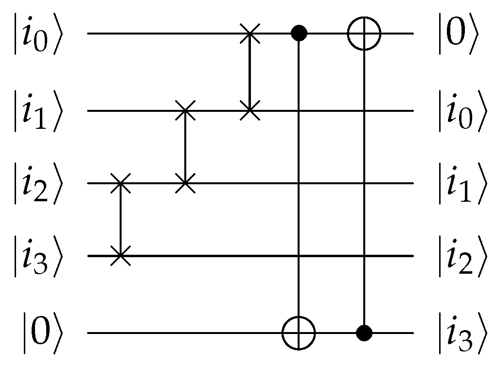
Step 3. We double the basis states of the first register: $|i_n{i}_{n-1}\dots i_1⟩\to |i_n{i}_{n-1}\dots i_{1}0mod{2}^n⟩=|i_{n-1}{i}_{n-2}\dots i_{1}0⟩$. This can be implemented directly by some swap gates, CNOT gates, and one auxiliary qubit.

In Figure 8, we present the circuit for doubling the basis state of four qubits. In this circuit, we want to double $|i_3{i}_2{i}_1{i}_0⟩$. By using one auxiliary qubit, we convert $|0i_3{i}_2{i}_1{i}_0⟩$ to $|i_3{i}_2{i}_1{i}_{0}0⟩$, and the output we need is $|i_2{i}_1{i}_{0}0⟩$. This means that $|i_3⟩$ on the auxiliary qubit is a garbage output. Here, we do not restore it to $|0⟩$ immediately, since its value will not affect the following steps. In Step 5, this auxiliary qubit will be restored to $|0⟩$ by uncomputation. Therefore, we omit this qubit in the description of our algorithm.

Figure 8. Quantum circuit for doubling.

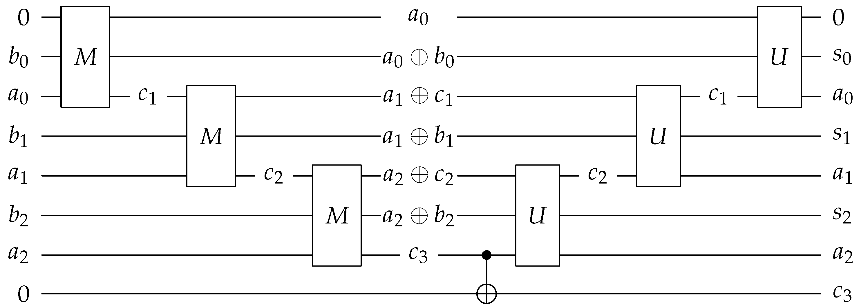
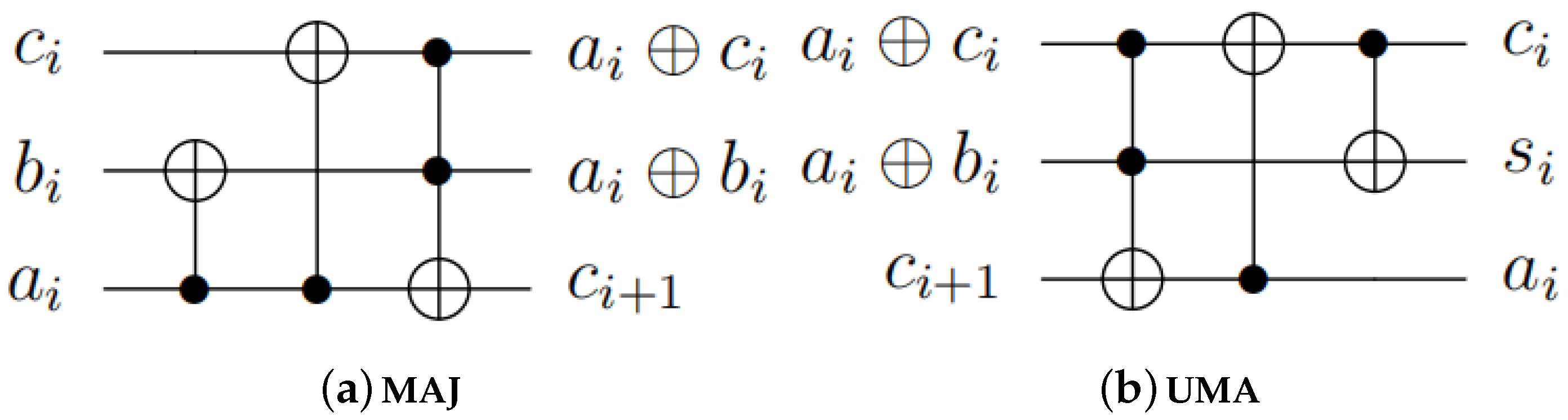
Step 4. We use the quantum adder in Figure 2 to apply the modular addition for the first two registers and store the result in the first register. It should be noted that the mod $2^n$ operation can be easily implemented by removing the operations that generate the highest carry in the quantum adder circuit. Therefore, the complexity of this step is $O(n)$.

Step 5. We run the quantum state extraction circuit in Figure 6 for the first and third registers in order to obtain the desired state. The complexity of this step is $O(n)$. The probability of obtaining this result is ${\displaystyle \frac{1}{2^n}}$. Since the state of the third register collapses to ${|0⟩}^{\otimes n}$, the normalized state is multiplied by a coefficient c, which is equal to $\sqrt{2^n}$ and can be cancelled out with the denominator. As the probability of the measurement outcome being ${|0⟩}^{\otimes n}$ is ${\displaystyle \frac{1}{2^n}}$, the quantum amplitude amplification algorithm can increase the probability to over $1-{\displaystyle \frac{1}{2^n}}$ with complexity $O(\sqrt{2^n})$. A detailed analysis of the measurement success probability will be presented in Section 4.

Step 6. We reverse the quantum arithmetic operations performed on the first register. This step has a complexity of $O(n)$.

Step 7. We apply the ${\mathbf{H}}^n$ transformation on the second register, and then measure the second register; the normalized state is multiplied by a coefficient $c^{\prime }$; the probability of the measurement outcome being ${|0⟩}^{\otimes n}$ is $O(\sqrt{N})$ in most case. A detailed analysis of the measurement success probability will be presented in Section 4.

Step 8. We return the quantum state of the three registers.

After organizing the complexity of the previous calculations, the overall complexity of the algorithm was determined to be $O(N{log}^2(N))$. Ultimately, we obtained a quantum state containing result information. Compared with classical results, the quantum state we obtained may have more applications, for example, when used in quantum convolutional neural networks.

In this section, we also present a new quantum representation method for circulant matrices, which is given through controlled matrices and related quantum states, with the expectation of having better applications.

3.2. The Second Algorithm

Theorem 3. 

There exists a quantum algorithm which computes the multiplication of the most circulant matrix and vector over $\mathbb{C}$ (or $\mathbb{R})$ with a probability of at least $1-{\displaystyle \frac{1}{N}}$ and complexity $O(\sqrt{N}{log}^{2}N)$, where N is the dimension of the matrix, and the proportion of the circulant matrix and vector combinations that can be effectively computed approaches 1 as the dimension increases.

We suppose that $\mathbf{a}={(a_0,a_1,\dots ,a_{n-1})}^{\top }$, and $\mathbf{A}$ is the corresponding circulant matrix for $\mathbf{a}$. Let $\mathbf{x}={(x_0,x_1,\dots ,x_{n-1})}^{\top }$; then, we have that computing $\mathbf{Ax}=\mathbf{b}$ is equivalent to computing ${\mathbf{FAF}}^{-1}\mathbf{Fx}=\mathbf{Fb}$. Moreover, we have ${\mathbf{FAF}}^{-1}=diag({\mathbf{F}}^{-1}\mathbf{a})$, so $\mathbf{Fb}$ can be computed by ${\mathbf{F}}^{-1}\mathbf{a}$ and $\mathbf{Fx}$. We can then use a quantum extraction circuit to extract the target state, and the whole algorithm is presented in Algorithm 2.

Algorithm 2 Multiplication of a circulant matrix and a vector

Input:  The quantum state $|a⟩|x⟩$ Output:  The quantum state    ${\displaystyle \frac{c}{\sqrt{(2^n)}}}{\sum }_{r=0}^{2^n-1}({\sum }_{j=0}^{2^n-1}{a}_j{x}_{j+r})|r⟩$  1: Apply the inverse quantum Fourier transform (${\mathrm{QFT}}^{†}$) to $|a⟩$ and the quantum Fourier transform (QFT) to $|x⟩$, then get the state $${\displaystyle \frac{1}{2^n}}\sum _{j=0}^{2^n-1}{a}_j(\sum _{k=0}^{2^n-1}{e}^{-2\pi ijk/2^n}|k⟩)\sum _{p=0}^{2^n-1}{x}_p(\sum _{q=0}^{2^n-1}{e}^{2\pi ipq/2^n}|q⟩).$$ (19)  2: Use the quantum extraction circuit in Figure 6 to extract our target state from the first two registers. Then, with some probability, we get the state $${\displaystyle \frac{c}{2^n}}\sum _{k=0}^{2^n-1}(\sum _{j=0}^{2^n-1}{a}_j{e}^{-2\pi ijk/2^n})(\sum _{p=0}^{2^n-1}{x}_p{e}^{2\pi ipk/2^n})|k⟩{|0⟩}^{\otimes n}.$$ (20)  3: Perform ${\mathrm{QFT}}^{†}$ on the first register, then get the state $${\displaystyle \frac{c}{{(2^n)}^{\frac{3}{2}}}}\sum _{k=0}^{2^n-1}(\sum _{j=0}^{2^n-1}{a}_j{e}^{-2\pi ijk/2^n})(\sum _{p=0}^{2^n-1}{x}_p{e}^{2\pi ipk/2^n})(\sum _{r=0}^{2^n-1}{e}^{-2\pi irk/2^n}|r⟩).$$ (21)  4: Return the quantum state $${\displaystyle \frac{c}{\sqrt{(2^n)}}}\sum _{r=0}^{2^n-1}(\sum _{j=0}^{2^n-1}{a}_j{x}_{j+r})|r⟩.$$ (22)

Here, we analyze the complexity of each step in detail.

Step 1. We apply ${\mathrm{QFT}}^{†}$ to $|a⟩$ and QFT to $|x⟩$. Obviously, the complexity of this step is $O(n^2)$.

Step 2. We use the quantum extraction circuit in Figure 6 to extract our target state from the first two registers. This step has a complexity of $O(n)$. When the measurement outcome is ${|0⟩}^{\otimes n}$, we obtain the target state. Since the state of the second register collapses to ${|0⟩}^{\otimes n}$, the normalized state is multiplied by a coefficient c. If the elements of vectors $\mathbf{a}$ and $\mathbf{x}$ (not normalized) are randomly chosen from $(-1,1)$ (over $\mathbb{R})$, or the ball (over $\mathbb{C}$) with a norm of 1, then, for most cases, the probability of the measurement outcome being ${|0⟩}^{\otimes n}$ exceeds ${\displaystyle \frac{1}{2N}}$. With a complexity of $O(\sqrt{N})$, the quantum amplitude amplification algorithm can increase this probability to at least $1-{\displaystyle \frac{1}{N}}$. Moreover, if the elements of $|a⟩$ and $|x⟩$ are randomly chosen from $(0,1)$, then, for most cases, the probability of obtaining ${|0⟩}^{\otimes n}$ exceeds ${\displaystyle \frac{1}{2}}$. The specific analysis will be discussed in the next section.

Step 3. We perform ${\mathrm{QFT}}^{†}$ on the first register, with a complexity of $O(n^2)$. Then, the amplitude of $|r⟩$ is

$$\begin{array}{cc}\hfill & {\displaystyle \frac{c}{{(2^n)}^{\frac{3}{2}}}}\sum _{k=0}^{2^n-1}(\sum _{j=0}^{2^n-1}{a}_j{e}^{-2\pi ijk/2^n})(\sum _{p=0}^{2^n-1}{x}_p{e}^{2\pi ipk/2^n})e^{-2\pi irk/2^n}\hfill \\ \hfill =& {\displaystyle \frac{c}{{(2^n)}^{\frac{3}{2}}}}\sum _{j=0}^{2^n-1}\sum _{p=0}^{2^n-1}\sum _{k=0}^{2^n-1}{a}_j{x}_p{e}^{{\displaystyle \frac{2\pi i(-j+p-r)k}{2^n}}}\hfill \\ \hfill =& {\displaystyle \frac{c}{{(2^n)}^{\frac{3}{2}}}}\sum _{j=0}^{2^n-1}\sum _{t=0}^{2^n-1}{a}_j{x}_{t+j}(\sum _{k=0}^{2^n-1}{e}^{{\displaystyle \frac{2\pi i(-j+(t+j)-r)k}{2^n}}})\hfill \\ \hfill & /*\mathtt{Substitute}\mathtt{p}\mathtt{with}\mathtt{t}+\mathtt{j}*/\hfill \\ \hfill =& {\displaystyle \frac{c}{{(2^n)}^{\frac{3}{2}}}}\sum _{j=0}^{2^n-1}\sum _{t=0}^{2^n-1}{a}_j{x}_{t+j}(\sum _{k=0}^{2^n-1}{e}^{{\displaystyle \frac{2\pi i(t-r)k}{2^n}}})\hfill \\ \hfill =& {\displaystyle \frac{c{2}^n}{{(2^n)}^{\frac{3}{2}}}}\sum _{j=0}^{2^n-1}{a}_j{x}_{j+r}={\displaystyle \frac{c}{\sqrt{(2^n)}}}\sum _{r=0}^{2^n-1}(\sum _{j=0}^{2^n-1}{a}_j{x}_{j+r})\hfill \end{array}$$

(23)

Step 4. We return the quantum state ${\displaystyle \frac{c}{\sqrt{(2^n)}}}{\sum }_{r=0}^{2^n-1}({\sum }_{j=0}^{2^n-1}{a}_j{x}_{j+r})|r⟩.$

In summary, the output of this algorithm is exactly the result of the circulant matrix–vector product given in the first algorithm. If the components of the vectors $\mathbf{a}$ and $\mathbf{x}$ (not normalized) are randomly selected from $(-1,1)$ (over $\mathbb{R}$), or the ball (over $\mathbb{C}$) with a norm of 1, then, for most cases, the complexity of this algorithm is $O(\sqrt{N}{log}^2(N))$. If the components of $|a⟩$ and $|x⟩$ are randomly selected from $(0,1)$, then the complexity of this algorithm is $O({log}^3(N))$, achieving exponential acceleration compared to classical algorithms.

4. Measurement Success Probability Calculation

In this section, we will present a detailed analysis of the probability of obtaining the target states after measurements in Algorithms Section 3.1 and Section 3.2. Here, we also omit the “mod N” symbol in the indices with $N=2^n$. The vectors $\mathbf{a}$ and $\mathbf{x}$ in this section are no longer normalized, and the conditions they satisfy will be given below.

For Algorithm 1, we have the following success rate of measurement in Step 4:

$$\begin{array}{cc}\hfill {\mathrm{Pr}}_{\mathrm{succ}}=& {\displaystyle \frac{{\sum }_{i=0}^{2^n-1}{\sum }_{j=0}^{2^n-1}(\frac{1}{\sqrt{2^n}}{a}_{i+j}{x}_{2i+j})(\frac{1}{\sqrt{2^n}}{\overline{a}}_{i+j}{\overline{x}}_{2i+j})}{{\sum }_{i=0}^{2^n-1}{\sum }_{j=0}^{2^n-1}{\sum }_{k=0}^{2^n-1}(\frac{1}{\sqrt{2^n}}{a}_{i+j}{x}_k)(\frac{1}{\sqrt{2^n}}{\overline{a}}_{i+j}{\overline{x}}_k)}}\hfill \\ \hfill =& {\displaystyle \frac{{\sum }_{i=0}^{2^n-1}{\sum }_{j=0}^{2^n-1}(\frac{1}{\sqrt{2^n}}{a}_{i+j}{x}_{2i+j})(\frac{1}{\sqrt{2^n}}{\overline{a}}_{i+j}{\overline{x}}_{2i+j})}{\frac{1}{2^n}{\sum }_{i=0}^{2^n-1}{\sum }_{j=0}^{2^n-1}{a}_{i+j}{\overline{a}}_{i+j}{\sum }_{k=0}^{2^n-1}{x}_k{\overline{x}}_k}}\hfill \\ \hfill =& \sum _{i=0}^{2^n-1}\sum _{j=0}^{2^n-1}({\displaystyle \frac{1}{\sqrt{2^n}}}{a}_{i+j}{x}_{2i+j})({\displaystyle \frac{1}{\sqrt{2^n}}}{\overline{a}}_{i+j}{\overline{x}}_{2i+j})\hfill \\ \hfill =& {\displaystyle \frac{1}{2^n}}\sum _{i=0}^{2^n-1}\sum _{t=0}^{2^n-1}{a}_{i+(t-i)}{x}_{2i+(t-i)}{\overline{a}}_{i+(t-i)}{\overline{x}}_{2i+(t-i)}\hfill \\ \hfill =& {\displaystyle \frac{1}{2^n}}\sum _{t=0}^{2^n-1}{a}_t{\overline{a}}_t(\sum _{i=0}^{2^n-1}{x}_{i+t}{\overline{x}}_{i+t})\hfill \\ \hfill =& {\displaystyle \frac{1}{2^n}}\hfill \end{array}$$

(24)

In Step 7, we have the state

$${\displaystyle \frac{1}{\sqrt{2^n}}}(\sum _{i=0}^{2^n-1}(\sum _{j=0}^{2^n-1}{a}_{i+j}{x}_{2i+j})|i⟩){|0⟩}^{\otimes n}{|0⟩}^{\otimes n}+|\perp ⟩,$$

(25)

where $|\perp ⟩$ is orthogonal to

$${\displaystyle \frac{1}{\sqrt{2^n}}}(\sum _{i=0}^{2^n-1}(\sum _{j=0}^{2^n-1}{a}_{i+j}{x}_{2i+j})|i⟩){|0⟩}^{\otimes n}{|0⟩}^{\otimes n},$$

(26)

so the success rate of measurement in Step 7 is ${\displaystyle \frac{1}{N}}({\sum }_{i=0}^{2^n-1}({\sum }_{j=0}^{2^n-1}{a}_{i+j}{x}_{2i+j})({\sum }_{j=0}^{2^n-1}{\overline{a}}_{i+j}{\overline{x}}_{2i+j}))$ and is $O(\sqrt{N})$ in most cases. We will use experiments later to illustrate.

For the probability calculation of Algorithm 2, unfortunately, we were unable to present an explicit formula. Therefore, we used experimental results to demonstrate that, for most matrices, we can effectively compute them in Algorithm 2. Our goal was to estimate the proportion of circulant matrix–vector combinations that our algorithm could effectively compute, in all circulant matrix–vector combinations. We randomly generated matrices and vectors by selecting elements from a given interval, and then used classical algorithms to calculate the required probability. We then recorded the proportion of circulant matrix–vector combinations that we could effectively compute, and observed how this proportion changes with the interval and dimension.

We first considered the circulant matrix–vector multiplication on $\mathbb{R}$ with the norm of the elements not exceeding d. Let $\mathbf{a}={(a_0,a_1,\dots ,a_{s-1})}^{\top }$ and $\mathbf{x}={(x_0,x_1,\dots ,x_{s-1})}^{\top }$ be two vectors with each component randomly chosen from $(-d,d)$. To satisfy the condition of quantum state, we need to normalize them, which gives

$${\mathbf{a}}^{\prime }={({\displaystyle \frac{a_0}{\sqrt{{\sum }_{i=0}^{s-1}{a}_i^2}}},{\displaystyle \frac{a_1}{\sqrt{{\sum }_{i=0}^{s-1}{a}_i^2}}},\dots ,{\displaystyle \frac{a_{s-1}}{\sqrt{{\sum }_{i=0}^{s-1}{a}_i^2}}})}^{\top }.$$

(27)

Moreover, we have

$${\mathbf{a}}^{\prime }={({\displaystyle \frac{\frac{a_0}{d}}{\sqrt{{\sum }_{i=0}^{s-1}{(\frac{a_i}{d})}^2}}},{\displaystyle \frac{\frac{a_1}{d}}{\sqrt{{\sum }_{i=0}^{s-1}{(\frac{a_i}{d})}^2}}},\dots ,{\displaystyle \frac{\frac{a_{s-1}}{d}}{\sqrt{{\sum }_{i=0}^{s-1}{(\frac{a_i}{d})}^2}}})}^{\top }.$$

(28)

If $a_i$ is randomly chosen from $(-d,d)$, then ${\displaystyle \frac{a_i}{d}}$ is randomly chosen from $(-1,1)$. Therefore, to simplify the computation, we can assume $d=1$. Similarly, we have

$${\mathbf{x}}^{\prime }={({\displaystyle \frac{x_0}{\sqrt{{\sum }_{i=0}^{s-1}{x}_i^2}}},{\displaystyle \frac{x_1}{\sqrt{{\sum }_{i=0}^{s-1}{x}_i^2}}},\dots ,{\displaystyle \frac{x_{s-1}}{\sqrt{{\sum }_{i=0}^{s-1}{x}_i^2}}})}^{\top }.$$

(29)

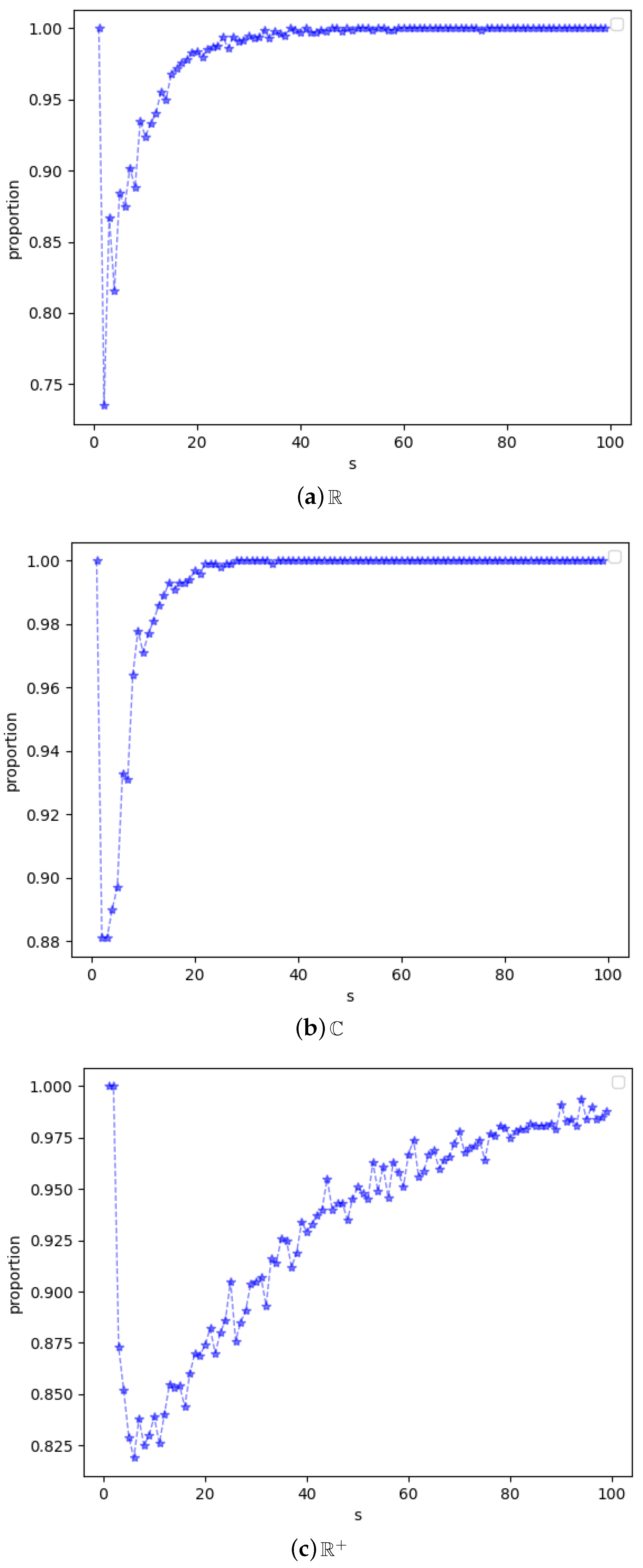
We consider the trend of the proportion of circulant matrix–vector combinations whose probability of obtaining the target state under this interval condition is greater than ${\displaystyle \frac{1}{2s}}$ as the dimension s varies. We randomly selected 1000 sets of $\mathbf{a}$ and $\mathbf{x}$ for each $s\in (1,2,\dots ,100)$ in the manner described above, and plotted Figure 9a based on the proportion of circulant matrix–vector combinations whose probability of obtaining the target state was greater than ${\displaystyle \frac{1}{2s}}$.

Figure 9. Proportion of valid circulant matrix–vector combinations on different domains with the change of dimension.

We notice that, as s increases, the values of the proportions from Figure 9a gradually approach 1. Therefore, we believe that our algorithm can effectively compute most of the circulant matrix–vector combinations on $\mathbb{R}$ with the norm of the elements in the matrix and vector not exceeding d, and the proportion of circulant matrix–vector combinations that can be effectively computed gradually approaches 1 as s increases. (It is obvious that the success rate is 1 when $s=1$).

Further, we consider the computation of circulant matrix–vector products with the norm of elements not exceeding 1 over $\mathbb{C}$, and discuss it in the same way as over $\mathbb{R}$, obtaining (b) of Figure 9. We also believe that our algorithm can effectively compute most circulant matrix–vector combinations over $\mathbb{C}$ with the elements’ norm in matrix and vector not exceeding 1, and the proportion of circulant matrix–vector combinations that can be effectively computed gradually approaches 1 as s increases.

When the elements are all in ${\mathbb{R}}^{+}$, we can obtain more exciting results compared to the first two domains under the same conditions. We raised the baseline probability of the target to ${\displaystyle \frac{1}{2}}$. The proportion of circulant matrices and vector combinations that satisfy the condition of having a probability greater than ${\displaystyle \frac{1}{2}}$ to measure the target state changes with the dimension s, as shown in Figure 9c. We find that this proportion also approaches 1 as s increases. Since ${\displaystyle \frac{1}{2}}$ is a constant, for matrix–vector combinations that satisfy the condition of having a probability greater than ${\displaystyle \frac{1}{2}}$, we need k measurements to get the target state with a probability of more than $1-{\displaystyle \frac{1}{2^k}}$.

Here, we also present some theoretical analysis results that we obtained. Let $|a⟩={\sum }_{k=0}^{N-1}{a}_k|k⟩,|x⟩={\sum }_{k=0}^{N-1}{x}_k|k⟩$; then, we have

$$F^{-1}|a⟩={\displaystyle \frac{1}{\sqrt{N}}}\sum _{j=0}^{N-1}(\sum _{k=0}^{N-1}{a}_k{e}^{{\displaystyle \frac{-2\pi ijk}{N}}})|j⟩,$$

(30)

$$F|x⟩={\displaystyle \frac{1}{\sqrt{N}}}\sum _{j=0}^{N-1}(\sum _{k=0}^{N-1}{x}_k{e}^{{\displaystyle \frac{2\pi ijk}{N}}})|j⟩,$$

(31)

$$(F^{-1}|a⟩)\otimes (F|x⟩)={\displaystyle \frac{1}{N}}\sum _{j_0=0}^{N-1}\sum _{j_1=0}^{N-1}[(\sum _{k=0}^{N-1}{a}_k{e}^{{\displaystyle \frac{-2\pi i{j}_{0}k}{N}}})(\sum _{k=0}^{N-1}{x}_k{e}^{{\displaystyle \frac{2\pi i{j}_{1}k}{N}}})]|j_0⟩|j_1⟩.$$

(32)

The coefficients of the basis state $|j_0⟩|j_1⟩$ in the aforementioned state can be denoted as $F_{j_0{j}_1}$. Let $F_t={\sum }_{j=0}^{N-1}{a}_j{x}_{j+t}$; then, we have

$$F_{kk}={\displaystyle \frac{1}{N}}\sum _{t=0}^{N-1}\sum _{j=0}^{N-1}{a}_j{x}_{j+t}{e}^{{\displaystyle \frac{2\pi itk}{N}}}={\displaystyle \frac{1}{N}}\sum _{t=0}^{N-1}{e}^{{\displaystyle \frac{2\pi itk}{N}}}{F}_t$$

(33)

The probability of obtaining the target state is

$$\begin{array}{cc}\hfill \sum _{k=0}^{N-1}{\left|F_{kk}\right|}^2& =\sum _{k=0}^{N-1}{F}_{kk}·\overline{F_{kk}}\hfill \\ \hfill & ={\displaystyle \frac{1}{N^2}}\sum _{k=0}^{N-1}(\sum _{t=0}^{N-1}{e}^{{\displaystyle \frac{2\pi itk}{N}}}{F}_t)(\sum _{t=0}^{N-1}{e}^{{\displaystyle \frac{-2\pi itk}{N}}}\overline{F_t})\hfill \\ \hfill & ={\displaystyle \frac{1}{N^2}}\sum _{k=0}^{N-1}(\sum _{t_0=0}^{N-1}\sum _{t_1=0}^{N-1}{e}^{{\displaystyle \frac{2\pi ik(t_0-t_1)}{N}}}{F}_{t_0}\overline{F_{t_1}})\hfill \\ \hfill & ={\displaystyle \frac{1}{N^2}}\sum _{t=0}^{N-1}(\sum _{k=0}^{N-1}{F}_t\overline{F_t})\hfill \\ \hfill & ={\displaystyle \frac{1}{N}}\sum _{t=0}^{N-1}{F}_t\overline{F_t}\hfill \end{array}$$

(34)

We look forward to someone providing an explicit formula for the probability distribution that correspond to the above expression when the entries of $|a⟩$ and $|b⟩$ satisfy some specific distributions.

If the approach modified by the HHL algorithm is used, we only need to calculate the multiplication instead of finding the inverse, so we have the state

$$\sqrt{{\displaystyle \frac{1}{{\sum }_{k=0}^{N-1}{({\lambda }_k^x)}^2{\widehat{{\lambda }_k}}^2{\mathbf{C}}^2}}}\sum _{k=0}^{n-1}\mathbf{C}{\lambda }_k^x\widehat{{\lambda }_k}|0⟩{|0⟩}^{\otimes m}|{\Lambda }_k⟩$$

(35)

where $\mathbf{C}$ is chosen to be $O(1)$ and $\widehat{{\lambda }_k}={\displaystyle \frac{{\lambda }_k}{{\lambda }_{max}}}$. Since ${\lambda }_k={\sum }_{j=0}^{N-1}{a}_j{\omega }^{-jk}\le {\sum }_{j=0}^{N-1}\left|a_j\right|\le \sqrt{N}$, ${\lambda }_{max}\le \sqrt{N}$. The complexity of quantum state extraction is $O({\sum }_{k=0}^{N-1}{({\lambda }_k^x)}^2{\widehat{{\lambda }_k}}^2{\mathbf{C}}^2)=O({\sum }_{k=0}^{N-1}|F_{kk}{|}^2)$. So, our second algorithm has the same probability of obtaining the target state as the approach modified by the HHL algorithm.

5. Quantum Convolution Computation

Quantum machine learning is a rapidly developing direction in quantum computing. Quantum convolutional neural networks have been proposed for image recognition and classical information classification. An example of a convolutional neural network was first proposed in [11]. For a typical image recognition problem, the input image undergoes convolution to generate a feature map, which is then classified. Rather than completing general convolution calculations like classical convolutional neural networks, existing convolutional neural networks use one of the following three approaches to entangle different qubits and improve parameters through optimization algorithms: use a fully random circuit, treat the circuit as a black box, and simply use CNOT gates. In contrast, we can use a quantum circuit to complete general convolution calculations.

Here, we focus on the problem of image recognition. First, we consider the conversion from classical information to quantum information. For this goal, Venegas-Andraca et al. [19] proposed a storage method based on a “qubit lattice”, where each pixel in an input image is represented by a qubit, requiring at least $2^n$ bits of storage. Le et al. [20] proposed an FRQI model, which associates pixel values and positions through the tensor product of quantum states. One qubit is used to encode pixel values, and color information is encoded in the probability amplitude. In [21], a NEQR model was proposed, which also associates pixel values and positions through tensor products, but uses d qubits to encode pixel values and encodes grayscale information in the basis state. In [22], a QImR model is proposed to encode 2D images into quantum pure states. In this model, pixel values are represented by the probability amplitude of the quantum state, and pixel positions are represented by the basis state of the quantum state.

We used the QImR model and assumed that we completed the representation of the image. We considered a one-dimensional convolution calculation and, below, we give the definition of convolution calculation.

$\mathbf{a}={(a_0,a_1,\dots ,a_{m-1})}^{\top }$ and $\mathbf{x}={(x_0,x_1,\dots ,x_{n-1})}^{\top }$ are sequences of length m and n, respectively. Their convolution is denoted as $\mathbf{h}=(h_0,h_1,\dots ,h_{m+n-2})$, where $h_i={\sum }_{j=0}^i{x}_j{a}_{i-j}$.

We set D to be the minimal integer satisfying $D\le m+n-1$ and $D=2^l$ for certain $l\in \mathbf{N}$. According to the definition of the QImR model, the quantum states $|a⟩$ and $|x⟩$ are given as follows: $|a⟩={\sum }_{i=0}^{D-1}{a}_i^{\prime }|i⟩$ and $|x⟩={\sum }_{i=0}^{D-1}{x}_i^{\prime }|i⟩$, where $a_i^{\prime }$ and $x_i^{\prime }$ satisfy

$$a_i^{\prime }=\left\{\begin{array}{cc}{\displaystyle \frac{a_i}{\sqrt{{\sum }_{j=0}^{m-1}{a}_j^2}}}\hfill & i\in [0,m-1]\hfill \\ 0\hfill & i\in (m-1,D)\hfill \end{array}\right.$$

(36)

$$x_i^{\prime }=\left\{\begin{array}{cc}{\displaystyle \frac{x_i}{\sqrt{{\sum }_{j=0}^{n-1}{x}_j^2}}}\hfill & i\in [0,n-1]\hfill \\ 0\hfill & i\in (n-1,D)\hfill \end{array}\right.$$

(37)

Their convolution is denoted as $|h⟩={\sum }_{i=0}^{D-1}{h}_i^{\prime }|i⟩$, where $h_i^{\prime }$ satisfies

$$h_i^{\prime }=\left\{\begin{array}{cc}{\displaystyle \frac{h_i}{\sqrt{({\sum }_{j=0}^{m-1}{a}_j^2)({\sum }_{k=0}^{n-1}{x}_k^2)}}}\hfill & i\in [0,m+n-2]\hfill \\ 0\hfill & i\in (m+n-2,D)\hfill \end{array}\right.$$

(38)

We plan to use circular matrix–vector multiplication to compute the convolution. The circular matrix corresponding to $|a⟩$ and required for convolution computation should be of the form

$$\mathbf{A}=\left(\begin{array}{ccccc}{a}_0^{\prime }& a_{D-1}^{\prime }& a_{D-2}^{\prime }& \dots & a_1^{\prime }\\ a_1^{\prime }& a_0^{\prime }& a_{D-1}^{\prime }& \dots & a_2^{\prime }\\ ⋮& ⋮& ⋮& \ddots & ⋮\\ a_{D-1}^{\prime }& a_{D-2}^{\prime }& a_{D-3}^{\prime }& \dots & a_0^{\prime }\end{array}\right)$$

(39)

It should be noted that the matrix here is the transpose of the matrix we previously introduced. Therefore, we need to construct $|a^{\prime }⟩$ from $|a⟩$, where $|a^{\prime }⟩={\sum }_{i=0}^{D-1}{a}_i^{\prime \prime }|i⟩$ and $a_i^{\prime \prime }=a_{D-i}^{\prime }$. We can first use apply an X gate to each qubit of the state $|a⟩={\sum }_{i=0}^{D-1}{a}_i^{\prime }|i⟩$ to obtain ${\sum }_{i=0}^{D-1}{a}_{D-1-i}^{\prime }|i⟩$, then apply $T^{-1}$ to obtain the target state $|a^{\prime }⟩$. The complexity of this part is $O({log}^{2}D)$.

Then, our two different multiplication algorithms can be used according to different result requirements. Compared with the classical one-dimensional convolution with a complexity of $O(DlogD)$, our algorithm can effectively accelerate it. The computation of two-dimensional convolution can also be extended in the same way.

In recent years, quantum neural networks have continuously developed, and improving their performance is a worthwhile research topic. For example, reference [23] proposes a new framework, ResQuNNs, as an improvement direction. The algorithm presented in this paper can improve the circuit of each layer and be combined with other methods to expect good results. On the other hand, quantum machine learning also poses significant challenges, such as the existence of plateaus. For this issue, improvements can be made in terms of framework and structure, as seen in references [24,25]. On the other hand, improvements can also be made to each layer of the circuit, combining the two aspects to further reduce the impact of high altitude.

6. Conclusions

We present two different algorithms for computing the multiplication of a circulant matrix and a vector. The two algorithms yielded results of different forms, and the appropriate algorithm can be chosen according to the computational needs. For most circulant matrices and vectors with elements in $\mathbb{C}$ or $\mathbb{R}$, our algorithm has a complexity of $O(\sqrt{N}{log}^{2}N)$ to compute their product. For most circulant matrices and vectors with elements in ${\mathbf{R}}^{+}$, we were able to reduce the complexity to $O({log}^{3}N)$, which achieves exponential acceleration compared to the classical complexity of $O(NlogN)$ for computing circulant matrix–vector multiplication.

Our algorithms are based on efficient quantum circuits for circulant matrices. With quantum circuits that can efficiently implement the quantum Fourier transforms, the multiplication of circulant matrices and vectors can be significantly accelerated. Compared to the HHL algorithm, our algorithms have the following advantages. First, we can complete the matrix operation through quantum circuits and corresponding vectors; hence, we no longer need to use quantum simulation to simulate the matrix to be calculated. Second, our complexity is no longer affected by the condition number, and we can present effective calculation for matrices with large condition numbers.

Furthermore, we have applied our approach to accelerate the basic convolution calculations for convolutional neural networks in machine learning. Our quantum circuit holds significant potential for applications in quantum machine learning, especially in convolutional neural networks.

In the success rate analysis of our second algorithm, we only presented some experimental results, which should also be expressed more clearly through probability theory in the future. Since different problems have different calculation intervals, finding more effective calculation intervals for this algorithm is also an interesting problem.