Scheduling for the Flexible Job-Shop Problem with a Dynamic Number of Machines Using Deep Reinforcement Learning

Abstract

The dynamic flexible job-shop problem (DFJSP) is a realistic and challenging problem that many production plants face. As the product line becomes more complex, the machines may suddenly break down or resume service, so we need a dynamic scheduling framework to cope with the changing number of machines over time. This issue has been rarely addressed in the literature. In this paper, we propose an improved learning-to-dispatch (L2D) model to generate a reasonable and good schedule to minimize the makespan. We formulate a DFJSP as a disjunctive graph and use graph neural networks (GINs) to embed the disjunctive graph into states for the agent to learn. The use of GINs enables the model to handle the dynamic number of machines and to effectively generalize to large-scale instances. The learning agent is a multi-layer feedforward network trained with a reinforcement learning algorithm, called proximal policy optimization. We trained the model on small-sized problems and tested it on various-sized problems. The experimental results show that our model outperforms the existing best priority dispatching rule algorithms, such as shortest processing time, most work remaining, flow due date per most work remaining, and most operations remaining. The results verify that the model has a good generalization capability and, thus, demonstrate its effectiveness.

1. Introduction

The job scheduling problem is a well-known and challenging optimization problem that occurs in many manufacturing and transportation scenarios [1]. For example, suppose a plant has several jobs to complete, and each job requires a sequence of tasks or operations. The plant also has some machines that can perform each task with a known processing time for each job. The goal is to assign the tasks to the machines so that the total completion time of all the jobs is minimized. This is a practical and important problem for efficient production.

A job scheduling problem consists of three basic elements: jobs, tasks, and machines. A job is a collection of one or more tasks, and a machine can process only one task at a time without interruption. Depending on the shop environments, job scheduling problems can be classified into different types, such as single-machine, parallel-machine, flow-shop, job-shop, and open-shop problems [2].

A single-machine problem involves multiple jobs, each with only one task. The goal is to find the optimal order of the jobs for a single machine. A parallel machine problem has multiple jobs, each with multiple tasks. A flow-shop problem has all jobs following the same sequence of tasks. A job-shop problem has different sequences of tasks for different jobs. This problem is NP-hard [3] and a major research topic in academia. An open-shop problem is similar to a job-shop problem, but the order of the tasks for each job does not matter.

A job-shop scheduling problem (JSSP) involves several jobs, each with a different number of tasks. Each task type has only one machine available. A flexible job-shop scheduling problem (FJSP) is a variant of the JSSP that allows for multiple machines for each task type. However, in some situations, new jobs may arrive or some machines may break down over time. This leads to a dynamic flexible job-shop scheduling problem (DFJSP), which is explained in detail in Section 3.

The job-shop scheduling problem (JSSP) is NP-hard, so finding optimal solutions for large problems is impractical. Therefore, priority dispatching rules (PDR) are often used, and many PDRs have been studied and compared in previous works [4]. However, deep reinforcement learning (DRL) methods have recently shown better performance than PDR methods for various DFJSPs.

Most of the existing DFJSP methods only consider dynamic job arrival, not dynamic machine availability. In this paper, we propose a scheduling method that can cope with dynamic machine availability and achieve efficient job scheduling with an end-to-end architecture, called the learning to dispatch (L2D) framework [5]. The L2D was initially designed for JSSP, which does not include any dynamic events. We adapt it to handle DFJSPs with dynamic machine availability. The contributions of this paper are as follows:

• We revise the end-to-end L2D framework to handle DFJSP with dynamic machine availability.
• We perform a simulation-based evaluation of the revised L2D algorithm.
• We enrich the node features in the graph representation of s DFJSP.
• We incorporate a baseline policy to compute rewards for improved performance.
• We open our source code for further research and development.

The outline of this paper is as follows: Section 2 covers the related work. Section 3 is the proposed approach to handle DFJSPs with a dynamic machine number. Section 4 contains the experiments and results, and Section 5 presents the conclusions and future research directions. To help the reader, we have included a list of acronyms in the Abbreviations.

2. Literature Review

According to Wikipedia, reinforcement learning (RL) is an area of machine learning to study how an agent takes actions in a dynamic environment to maximize the cumulative reward [6]. Recently, incorporating neural networks in RL agents has received lots of attention [7,8,9,10]. There are several types of RL algorithms based on different optimality criteria. One type is the value-based algorithms, such as Q learning [11], deep Q-learning (DQN) algorithm [12], and double deep Q-learning (DDQN) [13]. The Q-learning and DQN approaches have been widely used in production scheduling problems [14,15,16,17,18,19,20,21,22], as discussed below. Another type of RL algorithms is the actor–critic type and its variants, such as proximal policy optimization (PPO) [23]. The PPO algorithm has also been used in production scheduling problems [5,24,25,26].

Conventional Q-learning has been applied to production scheduling problems with success. Fonseca-Reyna et al. [14] used it for solving job-shop scheduling problems. They achieved better results in a shorter computing time. Shahrabi et al. [15] applied it to update the parameters of the variable neighborhood search algorithm, which is used as the scheduling algorithm for the studied dynamic job-shop scheduling problems with random job arrivals. Wang et al. [16] proposed a multi-agent approach for solving JSSP. They used a weighted Q-learning algorithm to determine the most suitable operation with better performance. Wang et al. [17] used two Q-learning agents for assembly job-shop scheduling, which consists of job-shop scheduling and an additional stage to assemble parts to jobs according to a bill of material. Their results showed that better results could be obtained than the single Q-learning and other scheduling rule approaches.

For applications of DQN to DFJSPs, Luo [18] showed promising results for random job arrivals by letting the DQN agent select dispatching rules. Luo et al. [19] subsequently used a two-hierarchy deep Q network to handle online multi-objective rescheduling for DFJSPs, such as new job arrivals and machine breakdowns. In their approach, the higher-level DQN determines the optimization goals, and the lower one selects the dispatching rules. Heger et al. [20] used Q-learning to handle DFJSPs with varying job arrival times and product flows, and they demonstrated the feasibility of their method in unseen scenarios. Turgut et al. [21] used the deep Q-network (DQN) to solve DFJSP with dynamic job arrivals, where the agent has to select and assign one of the waiting tasks to the first available machine. Their method outperformed the shortest processing time (SPT) and earliest due date (EDD), two conventional PDR methods. Chang et al. [22] used DDQN to solve a DFJSP with stochastic job arrivals and showed that their method outperformed existing RL and heuristic methods in dynamic scheduling problems.

Graph neural networks (GNNs) are a type of artificial neural networks that can process data that have a graph structure [27]. GNNs can learn from the graph data by using a message passing mechanism and update internal representations based on the local and global structures of the graph. A variant of the GNN is the graph isomorphism network (GIN), which is suitable for graph classification tasks [28]. Several studies have combined GIN and PPO to solve DFJSPs with a dynamic job arrival [5,24,25]. Zhang et al. introduced the L2D framework [5], which combines the graph neural network (GNN) and proximal policy optimization (PPO) to solve JSSP. They proposed a novel idea of using jobs and machines as the state space and letting the reinforcement-learning agent assign tasks based on the state representation. L2D learns the policy in an end-to-end manner without relying on predefined rules. A modified version of L2D open-source software can be found in [29]. Lei et al. [24,25] extended the L2D framework to handle dynamic job arrival problems. Their approach incorporated a high-level agent, based on double deep Q-networks (DDQN), to cache and dispatch the newly arrived jobs. Thus, a DFJSP can be transformed into static FJSPs and solved by the low-level L2D agent. Zhang et al. [26] introduced a multi-agent-based distributed scheduling architecture, which reduces the workload on the central server. They used a scheduling model based on the PPO algorithm, which can handle unpredictable events, such as new job arrivals and machine breakdowns.

From the above review, we know that most of the existing studies use reinforcement learning algorithms to select dispatch functions based on designed features [14,15,16,17,18,19,20,21,22]. However, this is not the ultimate goal that neural-network researchers are aiming for: an end-to-end architecture that can solve a problem [30]. By using an end-to-end architecture, the learning algorithm can adjust its internal representations to better fit the problem.

The end-to-end L2D model was originally proposed for solving the JSPP. Although it was later extended to solve the DFJSP with a stochastic job arrival, it did not address the dynamic change in the number of machines. In fact, only a few papers have ever considered the breakdown of a machine, let alone the dynamic number of machines. We believe that this problem has not been adequately investigated in the literature.

3. Proposed Approach

This section describes the proposed approach and all necessary materials. This section starts with the mathematical description of the DFJSP. It is followed by a Markov decision process, the graph representation of the states, the node features, the calculation of rewards, and the proposed approach.

3.1. Dynamic Flexible Job-Shop Scheduling Problem

Before we formally define the studied problem, we first describe the JSSP. A JSSP instance consists of a set of jobs $\mathit{J}=\left\{J_1,J_2,\cdots ,J_n\right\}$ and a set of machines $\mathit{M}=\left\{M_1,M_2,\cdots ,M_m\right\}$. Each job $J_i$ contains multiple tasks $O_{ij}$, $1\le j\le m_i$, where $m_i$ indicates the number of machines that $J_i$ needs to visit to complete the job. The size of a JSSP instance is expressed as |J| × |M|, where $|·|$ denotes the cardinality (i.e., the number of elements) of the set. The JSSP has three constraints: (i) each task $O_{ij}$ needs to be processed by a specified machine $M_k\in \mathit{M}$. (ii) Tasks $\left\{O_{i1},O_{i2},\cdots ,O_{i{m}_i}\right\}$ must be processed in order, expressed as $O_{i1}\to O_{i2}\to \cdots \to O_{i{m}_i},$ which is known as “precedence constraint”. (iii) Each machine can only process one task at a time, and the processing is non-preemptive.

For a specific task $O_{ij}$, its makespan is $c_{i,j}=s_{ij}+p_{ij}$, where $s_{ij}$ is the staring time of the task, and $p_{ij}\in \mathbb{N}$ is the processing time. The optimal solution of a JSSP instance is to minimize $c_{max}=\underset{i,j}{max}{c}_{ij}$.

The flexible job-shop scheduling problem (FJSP) allows for more than one machine for each task type. Let $\mathit{M}=\left\{{\mathit{M}}_1,{\mathit{M}}_2,\dots ,{\mathit{M}}_m\right\}$ be the set machine types, where each type ${\mathit{M}}_k$ has $l_k$ identical machines, i.e., ${\mathit{M}}_k=\left\{M_{k1},M_{k2},\dots ,M_{k{l}_k}\right\}$. Unlike the JSSP, $O_{ij}$ can now be processed by any machine in ${\mathit{M}}_k$, instead of one dedicated machine.

In this paper, we study the problem of dynamic machine numbers in the FJSP. We assume that the number of machines of each type follows a Poisson distribution and changes randomly over time. Therefore, the value $l_k$ will vary over time with an upper bound of $n_k$, i.e., $l_k\in \left\{1,2,\dots ,n_k\right\}$. The details of the Poisson distribution and the formula for increasing and decreasing the number of machines are given in Section 4.1.

3.2. Markov Decision Process for Scheduling JSSP

Before we describe the proposed approach, we first explain how to solve a JSSP by using a Markov decision process (MDP), which contains states and actions.

States. Let $\mathit{O}$ be the set of nodes containing tasks, let C be the set of directed arcs (conjunction) that connect two tasks based on the precedence constraints, and let D be the set of nondirectional edges (disjunctions) that connect two tasks that need the same machine for processing. We define the state $S_t$ of an MDP at step t as a graph $G=\left(\mathit{O},\mathit{C}{\displaystyle \cup }{\mathit{D}}_u\left(t\right),\mathit{D}\left(t\right)\right)$ that represents the solution up to t, where ${\mathit{D}}_u\left(t\right)\subseteq \mathit{D}$ is the set of edges that have been assigned a direction up to t, $\mathit{D}\left(t\right)$ is the set of the remaining $\mathit{D}$, and $t=\left\{0,1,\dots ,T\right\}$, where T is the maximum number of decision steps. Each node $O_{ij}$ has two features: the first feature ${\tilde{c}}_{i,j}$ is the lower bound of the makespan $c_{i,j}$ of the task, and the second feature is a binary indicator $I\left(O_{ij},S_t\right)\in \left\{0,1\right\}$, which is 1 if $O_{ij}$ has been scheduled before $S_t$, and 0 otherwise.

As an example, we use a simple JSSP instance, shown in Figure 1. The dummy nodes (begin and end) are omitted for simplicity. The instance has three jobs, each with three tasks. Each task is represented by a circle, and the color of the circle indicates the machine type (A, B, or C) required for the task. The solid arrows indicate the precedence constraints of the jobs. The two numbers above each node (task) are the features explained earlier. As shown in Figure 1, the first feature is the lower bound of its makespan of the task, which depends only on the precedence constraints, since no task has been scheduled yet.

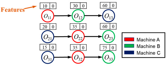
Figure 1. A simple JSSP instance.

Action. An action $a_t\in {\mathit{A}}_t$ is a task that can be scheduled at step t. The action space ${\mathit{A}}_t$ is a set whose elements are feasible tasks in the current state $S_t$. Feasible tasks are determined by the precedence constraints and the availability of the required machine. Figure 2a illustrates the action space of a JSSP in a specific state, $S_3$. Note that $O_{11}, O_{31}, O_{32}$are filled with purple color to indicate that they have been scheduled (as indicated by the $I\left(O_{ij},s_t\right)$ indicators in these nodes). Therefore, they will not be in the action space anymore. Feasible tasks are the ones that are ready to be processed for each job. For instance, $O_{22}$ is not a feasible task because $O_{21}$ has not been scheduled yet. All feasible tasks are filled with yellow color in Figure 2a, i.e., ${\mathit{A}}_3=\left\{O_{12}, O_{21}, O_{33}\right\}$.

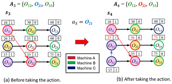
Figure 2. An example of state transition. A dash line shows the sequence of machine A in processing tasks. The red numbers indicate the changed feature values after taking the action. (a) Before taking the action. (b) After taking the action.

State Transition. When an action $a_t$ is selected in state $S_t$, the state transitions to $S_{t+1}$. This changes $D_u\left(t\right)$ in the graph $G$ and some node features accordingly. Figure 2b shows an example after the transition. When $a_3=O_{21}$. is chosen, machine C moves from $O_{31}$ to $O_{21}$to start processing, so an edge is directed from $O_{31}$ to $O_{21}$ in $D_u\left(t\right)$. The dashed lines in Figure 2b show the assignments of machines A (in red circles) and C (in blue circles) to tasks. Then, task $O_{21}$ and its successors $O_{22}$, $O_{23}$ (under precedence constraints) update their first features, as ${\tilde{c}}_{ij}=r_{ij}+p_{ij}$. If $a_t=O_{ij}$, then $r_{ij}=s_{ij}$, the start time of the task based on the machine availability. Otherwise, $r_{ij}$ is set as ${\tilde{c}}_{ij}$ of $O_{\left(i-1\right)j}.$ The second feature of $O_{21}$ is also set to 1. Note that ${\tilde{c}}_{ij}$ may be updated only based on ${\tilde{c}}_{i\left(j-1\right)}$; therefore, it is not the actual makespan of task $O_{ij}$.

3.3. Graph Representation for the Proposed Approach

To apply the L2D model, we first need to represent the problem as a graph. Recall that in the DFJSP instance, each task type has a dynamic number of identical machines. Therefore, each, $O_{ij}$has multiple parallel subtasks $O_{ijq}\in O_{ij}, 1\le j\le m_i$, $1\le q\le l_k$. Each $O_{ijq}$ has a processing time $p_{ij}\in \mathbb{N}$ for all $q$. A task $O_{ijq}$ is considered scheduled if any of the subtasks is scheduled.

We define the initial state $S_0$ of the graph $G=\left(\mathit{O},\mathit{C}, \mathit{D}\right)$ with $\mathit{O}, \mathit{C}$, and $\mathit{D}$ defined previously. If $O_{i\left(j+1\right)q }$ exists, then $O_{ijq}\to O_{i\left(j+1\right)q},1\le q\le l_k$. This represents the precedence constraint between nodes. Each node $O_{ijq}$can only be processed by one specific machine $M_{kr}$. If the number of machines changes, for example, if machine $M_{kr}$ is removed, then we need to remove the set of nodes $\left\{O_{1jq}, O_{2jq}\dots ,O_{ijq}\right\}$ that are processed by $M_{kr}$ from the graph G, and also the precedence constraints related to these nodes. The same idea applies when adding a new machine to a type.

Figure 3a illustrates the initial state $S_0$ of the problem. There are three machine types: ${\mathit{M}}_1$ with one machine $\left\{M_{11}\right\}$, ${\mathit{M}}_2$ with two machines $\left\{M_{21},M_{22}\right\}$, and ${\mathit{M}}_3$ with three machines $\left\{M_{31}, M_{32}, M_{33}\right\}$. Each task of each job has multiple parallel nodes in the graph, representing the same task processed by different machines. These parallel nodes are considered as one task, and only one of them can be scheduled. The other parallel nodes will be in the graph, but become invalid actions, once one of them is scheduled. It is possible to remove the unused parallel nodes. However, our preliminary experiments show that keeping them in the graph achieves better performance. The solid arrows indicate the precedence constraints between different tasks, as shown in Figure 3a. The construction of $D_u\left(t\right)$ follows the same procedure as before.

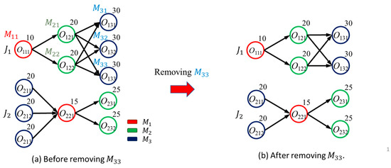
Figure 3. Removing a machine in the DFJSP. (a) Before removing $M_{33}.$ (b) After removing $M_{33}.$

Suppose we randomly remove one machine from $M_3$, for example, $M_{33}$. Then, we also have to delete all the nodes that $M_{33}$ processed, as Figure 3b illustrates. However, this representation has a drawback: the graph will grow very large as the number of machines increases.

3.4. Proposed Features for Each Node

As mentioned in Section 3.2, the original L2D approach uses only two features. However, these features are not enough to differentiate the states of the same task on different machines. Hence, we introduce a third feature $s_{ijq}$ as the actual start time of the task $O_{ijq}$. We compute it as follows:

$$s_{ijq}=\max \left({\tilde{c}}_{ijq}-p_{ij}, s\left(M_{kr}\right)\right),$$

(1)

where $s\left(M_{kr}\right)$ is the start time of machine $M_{kr}.$ The start time of the task depends on both the end time of the previous task and the start time of the machine. The task can begin processing only when the previous task is completed and the machine is free. Thus, the actual start time of the task is the maximum of these two values.

Let us use Figure 4 as an example. The rightmost feature is the new feature we added. Suppose the current state has an action space of ${\mathit{A}}_1=\left\{O_{121}, O_{122}\right\}$, and $M_{21}$ is busy with other tasks until time 20. Then, $M_{21}$ can start processing $O_{121}$ at time 20. $M_{22}$ is idle, so it can start processing $O_{122}$ at time 0. Without the third feature, we cannot tell the difference between the feature values of $O_{121}$ and $O_{122}$. Using (1), we get $s_{121}=$ $\max \left(30-20, 20\right)=20$, where $p_{12}=20.$Similarly, we get $s_{122}=\max \left(30-20, 0\right)=10$. Thus, we can distinguish the same task on different machines with the third feature.

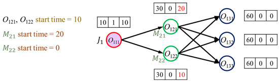
Figure 4. Example of calculating features.

3.5. State Transition for the Proposed Approach

We use Figure 5 to demonstrate the state transition of our approach. Let the action space of state $S_t$ be $A_t=\left\{O_{111}, O_{211}, O_{212}, O_{213}\right\}$, the leftmost nodes on Figure 5. If we choose $O_{211}$ as the action, the action space becomes ${\mathit{A}}_{t+1}=\left\{O_{111}, O_{221}\right\}$, and we cannot select $O_{212}$ and $O_{213}$. The action also updates the features, as the right part of Figure 5 shows. Note that we update $s_{ijq}$ and $I\left(O_{ijq},S_t\right)$ according to Section 3.3, and we mark the changed feature values in red.

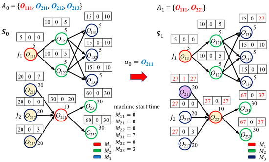
Figure 5. Example of state transition of the proposed approach. Red numbers indicate the change of the features.

3.6. Reward in the Proposed Approach

Following Duan et al. [31], who used a REINFORCE algorithm with a deterministic greedy rollout to train the agent, we implemented a Baseline policy to compute the reward. Figure 6 illustrates the reward calculation process. We start with random weights to generate an agent with a Baseline policy ${\mathrm{P}}_{{\mathsf{\theta }}^{BL}}$. We want to learn a reinforcement-learning policy ${\mathrm{P}}_{\mathsf{\theta }}$. At the start of an episode, we use ${\mathrm{P}}_{{\mathsf{\theta }}^{BL}}$ to find $D_{u,{\mathrm{P}}_{{\mathsf{\theta }}^{BL}}}\left(T\right)$ and makespan $c_{max,{\mathrm{P}}_{{\mathsf{\theta }}^{BL}}}$ of a training instance. Then, we iterate time step t from 0 to T and let actions $a_0,\cdots ,a_t$ be determined by ${\mathrm{P}}_{\mathsf{\theta }}$ and the remaining actions $a_{t+1},\cdots ,a_T$ by ${\mathrm{P}}_{{\mathsf{\theta }}^{BL}}$ to find the makespan of the training instance, denoted as $c_{max,{\mathrm{P}}_{\mathsf{\theta }}\left(S_t\right)}$. We calculate the reward as $R\left(a_t,S_t\right)=c_{max,{\mathrm{P}}_{\mathsf{\theta }}\left(S_t\right)}-c_{max,{\mathrm{P}}_{\mathsf{\theta }}\left(S_t+1\right)}$. Thus, if ${\mathrm{P}}_{\mathsf{\theta }}$ selects a better action $a_{t+1}$, $c_{max,{\mathrm{P}}_{\mathsf{\theta }}\left(S_t+1\right)}$ will decrease, and the reward is positive. At the end of each episode, if $c_{max,{\mathrm{P}}_{{\mathsf{\theta }}^{BL}}}>c_{max,{\mathrm{P}}_{\mathsf{\theta }\left(S_T\right)}}$, we replace parameters of the baseline policy ${\mathsf{\theta }}^{BL}$ with $\mathsf{\theta }$ and begin the next episode training.

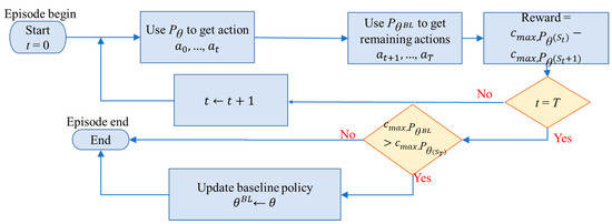
Figure 6. Proposed reward calculation.

3.7. Network Model of the Proposed Approach

L2D architecture. Our method follows the same overall architecture as L2D [5], which has two components: state embedding and learning policy, as shown in Figure 7. State embedding maps the graph G at $S_t$to an internal representation using a graph isomorphism network (GIN). The GIN can handle graphs with varying numbers of nodes and edges, but each node must have the same number of features. L2D uses a PPO algorithm as the learning policy to evaluate and select the best action. For brevity, we skip the details of the L2D method. Please see [5] for more information.

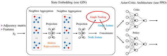
Figure 7. Architecture of L2D.

The proposed approach. The L2D framework was initially developed for JSSP, which does not contain any dynamic events. Hence, it uses only two features per node, and its reward function was merely the difference in the makespan in two successive steps. To adapt the L2D framework to our problem, we need to tackle the dynamic problem with a better reward design.

Figure 8 illustrates our proposed approach. We focus on the implementation details of our model, rather than the theoretical background, for brevity. The source code of our model is given in the Supplementary Materials section of this paper. As Figure 8 shows, the first step, neighboring, performs a matrix multiplication of the adjacency matrix and the feature matrix. The feature matrix has a size of $n\times f$, where $n$ is the number of nodes in the graph and $f=3$ is the number of features in one node. The graph itself is represented by an adjacency matrix of size $n\times n$ with the rows indicating the end nodes and the columns indicating the start nodes. Then, we divide each row of the product matrix of size $n\times f$ by the degree of the node to achieve average pooling.

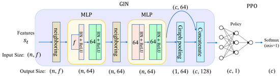
Figure 8. Proposed approach.

We use two multi-layer perceptrons (MLPs) to implement the GIN. Each MLP is a fully connected feedforward network with a rectified-linear-unit (ReLU) activation function and 64 hidden units. The first MLP takes inputs of size $f\times 1$, so we need to collect the outputs n times to get the full output of size $n\times 64$. This enables the network to handle graphs with varying sizes, such as those with a dynamic number of machines. The second neighboring layer performs the same operations mentioned previously.

The second neighboring layer repeats the same steps as the input neighboring layer, except that it uses the output of the first MLP as the feature matrix. The graph pooling performs average pooling to aggregate information from multiple nodes into one. However, it only averages the nodes in the action list ${\mathit{A}}_t$ ($\mathrm{i}.\mathrm{e}.,\left|{\mathit{A}}_t\right|=c$). This layer has an output size of $1\times 64$. The concatenating layer concatenates the average-pooled outputs and the unaveraged outputs. To be able to concatenate, the outputs of the average pooling is copied $c$ times to form a $c\times 64$ matrix.

The PPO network is also a multi-layer feedforward network. It takes 128 input values, has 64 hidden units, and produces one output value at a time, corresponding to the current node in the action list ${\mathit{A}}_t$. Suppose that we feed the first row of the concatenated outputs to the PPO network and get $y_1$. Then, we feed the second row and get $y_2$. We repeat this process until we get $y_c$. Next, we apply a softmax function to all ${\mathrm{y}}_i$. Since the PPO network only computes softmax for valid actions, this is equivalent to using an action mask to exclude invalid actions [32].

To handle the dynamic change of machine number, we have to reconstruct the graph and the node features whenever a machine goes online or offline at time $t=t_0$. We also have to recalculate $c_{max,{\mathrm{P}}_{{\mathsf{\theta }}^{ BL}}}$ from $t=0$, using the previously chosen actions for $t<t_0$. To train the PPO with a variable number of machines, we first collect the values of the surrogate objective, the advantage estimator, and the entropy over the entire episode, and then apply backpropagation with the collected values.

4. Experiments and Results

We designed two experiments to evaluate our proposed approach. The first experiment compared our method with existing PDR methods. The second experiment tested the generalization ability of our approach, using the trained model to solve DFJSP instances of various sizes.

4.1. Experimental Setup

We randomly generated all the datasets used in the experiments. The processing time of each task ranged from 1 to 99. We denoted the size of each problem as $\left|\mathit{J}\right|\times \left|\mathit{M}\right|$. Initially, each type of machines was set to $\left|{\mathit{M}}_i\right|=n\pm 20\%,1\le i\le \left|\mathit{M}\right|$ with a minimum of 1, where $n={\log }_2\left(\left|\mathit{J}\right|/\left|\mathit{M}\right|\right)+1$ is the average number of machines in all types. The number of processes (i.e., adding or removing a machine) follows a non-standard asymmetric random walk, with the step time inter-arrivals following an exponential distribution with mean $\left(\frac{1}{\lambda }\right),$ where

$$\lambda =\frac{\left|\mathit{J}\right|·\left|\mathit{M}\right|}{n},$$

(2)

And where $·$ is the multiplication. If an event occurs, a machine of type ${\mathit{M}}_i$ has a probability of $\frac{U_{{\mathit{M}}_i}-C_{{\mathit{M}}_i}}{U_{{\mathit{M}}_i}-L_{{\mathit{M}}_i}}$ to add a machine and $1-\frac{U_{{\mathit{M}}_i}-C_{{\mathit{M}}_i}}{U_{{\mathit{M}}_i}-L_{{\mathit{M}}_i}}$ to remove a machine, where $U_{{\mathit{M}}_i}$ is the maximum number of machines of type ${\mathit{M}}_i$, $C_{{\mathit{M}}_i}$ is the current number of machines of type ${\mathit{M}}_i$, and $L_{{\mathit{M}}_i}$ is the lower-bound of the machine, i.e., 1. We randomly generated a DFJSP instance for each of the 10,000 training episodes. The test set contained 30 DFJSP instances.

The experiments were conducted through computer simulations. The programming language was Python, and the deep learning package was PyTorch. The equipment and software versions are listed in Table 1 and Table 2.

Table 1. Equipment specifications.

	Computer 1	Computer 2	Computer 3
Processor	Intel Core i7-9700 3.00 GHz × 8	Intel Core i7-7700 3.60 GHz × 8	Intel Core i7-4770 3.40 GHz × 8
Memory	16 GB	40 GB	16 G
OS	Windows 10	Ubuntu 18.04	Ubuntu 18.04

Table 2. Software version.

Library	Version
PyTorch	1.13.1
OR-Tools	9.6.2534
Python	3.10

4.2. Experiment One

We compare our method with four traditional PDRs: Shortest Processing Time (SPT), Most Work Remaining (MWKR), Flow Due Date per Most Work Remaining (FDD/MWKR), and Most Operation Remaining (MOPNR). SPT is a common PDR in the industry, whereas the others are the best PDRs on the Taillard test set [2]. This experiment evaluated the performance of these four PDRs and our method.

In DFJSPs, each task has multiple machine options. However, the PDRs we compared only had priority rules for tasks, not for machines. So, we introduced a second rule for these PDRs: pick the machine that can start the earliest. This rule enhances the performance of the PDRs.

We trained two models with FJSP datasets of sizes 6 × 3 and 15 × 5 and tested them on the same-sized test sets. We compared our models with four conventional PDRs and OR-Tools [33], a tool provided by Google for solving combinatorial optimization problems. We limited the OR-Tools to have a maximum execution time of 600 s, as it took too long to solve some instances. Table 3 shows the simulation results, where “Gap” indicates the performance difference between OR-Tools and each method, “Time (s)” is the average execution time of a method, and “Reschedule” is the average number of dynamic events. Dynamic events change the number of online machines, requiring the rescheduling of all the work after that point. If a machine to be removed is processing a task at that time, the task needs to be interrupted and reassigned to another machine of the same type. We used our approach to explore all dynamic events before OR-Tools solved the problem, so it knew the number of online machines at any time. Therefore, OR-Tools did not need to handle any dynamic events.

Table 3. Simulation results for experiment one.

Size	Avg. ${\mathit{M}}_{\mathit{i}}$		SPT	MWKR	FDD/MWKR	MOPNR	Prop.	OR-Tools
6 × 3	2	Makespan	507.8	375.7	362.3	368.0	342.5	313
		Gap	62.2%	20.0%	15.8%	17.6%	9.4%	0.0%
		Time (s)	0.037	0.026	0.025	0.024	0.086	0.081
		Reschedule	9.4	6.5	5.9	5.9	5.3	-
15 × 5	2.58	Makespan	1373.1	736.6	704.7	717.7	679.7	560.6
		Gap	144.9%	31.4%	25.7%	28.0%	21.2%	0.0%
		Time (s)	1.501	0.768	0.730	0.690	1.655	13.445
		Reschedule	47.7	24.5	22.7	22.0	21.1	-

Table 3 shows that our method outperforms the existing PDRs. Our method is slower than PDRs, but the execution time is reasonable. However, OR-Tools takes much longer to solve larger problems. We notice that the Gaps of the compared methods grow much larger in bigger problems. We believe this is because changing the number of machines dynamically causes some machines to be idle whenever rescheduling happens. Recall that a bigger problem has more machines of each type, and, therefore, a higher rescheduling rate according to (2).

4.3. Experiment Two

We tested the generalization ability of our model by using the $15\times 5$ model trained in the first experiment to solve DFJSP instances with different sizes of jobs and machines. Table 4 shows the results, where we added a row “ORT < 600” to show the percentage of instances that OR-Tools could solve within 600 s. Table 4 reveals that OR-Tools takes much longer time to solve larger problems. Thus, OR-Tools is not suitable for large-scale problems. In fact, for $30\times 10$ and $60\times 5$ problems, the “ORT < 600” value was zero, indicating unoptimized solutions.

Table 4. Simulation results for experiment two.

Size	Avg. ${\mathit{M}}_{\mathit{i}}$		SPT	MWKR	FDD/MWKR	MOPNR	Prop.	OR-Tools
6 × 6	1	Makespan	1116.9	661.1	628.0	646.3	570.3	489.5
		Gap	128.2%	35.1%	28.3%	32.0%	16.5%	0.0%
		Time (s)	0.014	0.014	0.013	0.013	0.062	0.034
		Reschedule	0.0	0.0	0.0	0.0	0.0	-
		ORT < 600						100%
15 × 10	1.58	Makespan	3391.2	1333.3	1279.6	1240.2	1209.3	918.4
		Gap	269.3%	45.2%	39.3%	35.0%	31.7%	0.0%
		Time (s)	21.757	7.613	7.173	6.740	16.921	124.383
		Reschedule	229.7	87.5	83.0	78.6	76.6	-
		ORT < 600						100%
30 × 10	2.58	Makespan	4249.8	1613.9	1532.9	1493.6	1466.1	1358.0
		Gap	212.9%	18.8%	12.9%	10.0%	8.0%	0.0%
		Time (s)	75.657	25.667	24.342	23.099	34.357	600.000
		Reschedule	318.9	117.8	111.1	104.7	103.7	-
		ORT < 600						0%
60 × 10	3.58	Makespan	6327.3	2301.9	2229.7	2107.1	2086.2	4490.6
		Gap	40.9%	−48.7%	−50.3%	−53.1%	−53.5%	0.0%
		Time (s)	449.958	162.277	150.711	140.851	203.364	600.000
		Reschedule	346.3	122.5	118.6	109.9	109.6	-
		ORT < 600						0%

Table 4 also shows that our method outperforms the PDRs, and even OR-Tools, on $60\times 10$ problems. The performance gap between our method and the PDRs does not shrink much as the problem size grows, suggesting that our method generalizes well.

4.4. Complexity and Execution Time

This subsection briefly discusses the execution time of the proposed approach. The training phase took a few hours for the proposed approach. The training time is not very important in actual application for two reasons. First, the scheduling agent can generalize its ability to different problem sizes than the training one, so the training is not urgent, and we can train the model offline at spare time. Second, the training time depends on the number of training episodes. We trained the models in 10,000 training episodes in the experiments, but the loss function reached the floor quickly within 5000 episodes. Therefore, we can reduce the training time by cutting the number of training episodes.

We have already presented the results of the execution time for test cases in Table 3 and Table 4. The execution time is not linearly related to the problem size ($\left|\mathit{J}\right|·\left|\mathit{M}\right|)$. The L2D is a cascade of the GIN and PPO agent, which are both MLPs. The complexity of the L2D, thus, depends on the number of input vectors to the GIN. The number of input vectors equals the number of nodes in the graph. The number of nodes changes when a machine goes online or offline. For example, Figure 9 shows that removing two machines in a simple problem eliminates four nodes in the graph. The adjacency matrix (each row is an input vector to the GIN) needs to be rebuilt after adding or removing nodes. It is hard to estimate the complexity of rebuilding the adjacency matrix, so we cannot provide a theoretical complexity analysis of the proposed approach.

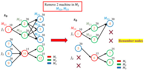
Figure 9. Removing two nodes. Note that a renumbering of nodes is necessary after the removal of machines for generating the adjacency matrix.

We observe that the MOPNR has the shortest execution time among the compared approaches, while MRWK and FDD/MWKR also have a low execution time, slightly higher than the MOPNR. The proposed approach needs relatively more computing time but less than twice the execution time of the MOPNR. The longer execution time is a drawback, but for moderate-sized problems, such as $30\times 10$, the time difference is only about 10 s.

Finally, the DFJSP is an NP-hard problem [3], so finding the optimal solution for a large-sized problem is practically impossible. The OR-Tools needs a very long execution time to find a good solution for a large-sized problem, such as $60\times 10$. As a result, it cannot provide an acceptable solution within a reasonable time, such as 600 s, as Table 4 shows. In contrast, the other methods can find better solutions in about 200 s. Therefore, OR-Tools is only suitable for small problems or problems that do not need fast rescheduling results.

5. Discussions

Despite the success of the proposed approach, it has some limitations and implications. First, we generated the simulation data artificially, not from actual industry data. Although using artificial data in simulations is common [5,22], it still introduces uncertainty when applying the proposed approach to a real problem. For example, the simulation assumes that a certain distribution governs the online or offline status of available machines. This may not be realistic, as planned machine maintenance and other factors can affect the availability. Making artificial data more realistic is a challenging problem.

Second, Table 4 shows that the proposed approach loses its edge over conventional approaches (in terms of % gap) when the number of machines in each type increases (i.e., Avg.${\mathit{M}}_i$). This phenomenon makes sense. More machines in each machine type give the algorithm more flexibility to make acceptable (or suboptimal) scheduling without too many constraints. Therefore, we need more studies to know how to train an agent that can perform better with larger problems and a higher Avg.${\mathit{M}}_i$.

6. Conclusions

The DFJSP with dynamic machine availability has been rarely investigated in previous studies, as most studies have focused on the dynamic job arrival. Moreover, many newly developed algorithms used RL algorithms to select dispatching rules, making it hard for learning-based improvement. In this paper, we propose a framework to tackle this issue based on the modified end-to-end L2D framework to minimize the makespan. By using a dynamic graph representation with a GIN, our framework can directly handle the dynamic number of available machines within the framework. We also use an RL agent network trained with PPO to select the task to be scheduled. By adding additional node features and improved reward calculation, our method outperforms the traditional PDRs, such as SPT, MWKR, FDD/MWKR, and MOPNR, under the dynamic rules we adopted, and it generalizes well to different sizes of jobs and machines. To facilitate the academic research on the proposed framework, the experimental code is publicly available.

From the experimental results, we observe that the proposed approach gradually loses its advantage as the number of available machines in each type increases. To improve this situation, we plan to add more features, such as those related to the number of machines, to enhance the RL agent’s ability to allocate the same type of machines. Moreover, the features may also include machine average utilization rate and task delay ratio to further improve the performance of the method. Furthermore, in the current method, the DFJSP dynamic events only affect the graph structure. Therefore, the agent is not aware of the occurrence of the dynamic event, and, thus, cannot learn the scheduling rules more efficiently. It is worthwhile to investigate the performance improvement by adding an event indicator to the feature set, such as the time span since the last event or the type of event, to enable the agent to learn the appropriate scheduling rules according to the indicator.

Currently, we only aim to minimize the makespan. In real working plants, other goals are also important, and we can explore different objective functions to meet the production goals, such as the work load balance between the machines and the product profit obtained within the time. With such an exploration, we believe that the proposed approach can be a useful tool for the manufacturing industry to solve various problems.

References

- Rinnooy Kan, A.H.G. Machine Scheduling Problems: Classification, Complexity and Computations; Springer: New York, NY, USA, 1976. [Google Scholar]
- Allahverdi, A. The third comprehensive survey on scheduling problems with setup times/costs. Eur. J. Oper. Res. 2015, 246, 345–378. [Google Scholar] [CrossRef]
- Job-Shop Scheduling. Available online: https://en.wikipedia.org/wiki/Job-shop_scheduling#NP-hardness (accessed on 18 December 2023).
- Sels, V.; Gheysen, N.; Vanhoucke, M. A comparison of priority rules for the job shop scheduling problem under different flow time-and tardiness-related objective functions. Int. J. Prod. Res. 2012, 50, 4255–4270. [Google Scholar] [CrossRef]
- Zhang, C.; Song, W.; Cao, Z.; Zhang, J.; Tan, P.S.; Chi, X. Learning to Dispatch for Job Shop Scheduling via Deep Reinforcement Learning. In Proceedings of the Advances in Neural Information Processing Systems, Vancouver, BC, Canada, 6–12 December 2020. [Google Scholar]
- Sutton, R.S.; Barto, A.G. Reinforcement Learning: An Introduction, 2nd ed.; MIT Press: Cambridge, MA, USA, 2018. [Google Scholar]
- Arulkumaran, K.; Deisenroth, M.P.; Brundage, M.; Bharath, A.A. Deep Reinforcement Learning: A Brief Survey. IEEE Signal Process. Mag. 2017, 34, 26–38. [Google Scholar] [CrossRef]
- Schmidhuber, J. Deep Learning in Neural Networks: An Overview. Neural Netw. 2015, 61, 85–117. [Google Scholar] [CrossRef] [PubMed]
- Krizhevsky, A.; Sutskever, I.; Hinton, G.E. ImageNet Classification with Deep Convolutional Neural Networks. Commun. ACM 2017, 60, 84–90. [Google Scholar] [CrossRef]
- Sierla, S.; Ihasalo, H.; Vyatkin, V. A Review of Reinforcement Learning Applications to Control of Heating, Ventilation and Air Conditioning Systems. Energies 2022, 15, 3526. [Google Scholar] [CrossRef]
- Watkins, C.J.C.H.; Dayan, P. Q-learning. Mach. Learn. 1992, 8, 279–292. [Google Scholar] [CrossRef]
- Mnih, V.; Kavukcuoglu, K.; Silver, D.; Rusu, A.A.; Veness, J.; Bellemare, M.G.; Graves, A.; Riedmiller, M.; Fidjeland, A.K.; Ostrovski, G.; et al. Human-level Control through Deep Reinforcement Learning. Nature 2015, 518, 529–533. [Google Scholar] [CrossRef] [PubMed]
- van Hasselt, H.; Guez, A.; Silver, D. Deep Reinforcement Learning with Double Q-Learning. In Proceedings of the AAAI Conference on Artificial Intelligence, Phoenix, AZ, USA, 12–17 February 2016. [Google Scholar]
- Fonseca-Reyna, Y.C.; Martinez, Y.; Rodríguez-Sánchez, E.; Méndez-Hernández, B.; Coto-Palacio, L.J. An Improvement of Reinforcement Learning Approach to Permutational Flow Shop Scheduling Problem. In Proceedings of the 13th International Conference on Operations Research (ICOR 2018), Beijing, China, 7–9 July 2018. [Google Scholar]
- Shahrabi, J.; Adibi, M.A.; Mahootchi, M. A reinforcement learning approach to parameter estimation in dynamic job shop scheduling. Comput. Ind. Eng. 2017, 110, 75–82. [Google Scholar] [CrossRef]
- Wang, Y.-F. Adaptive job shop scheduling strategy based on weighted Q-learning algorithm. J. Intell. Manuf. 2018, 31, 417–432. [Google Scholar] [CrossRef]
- Wang, H.; Sarker, B.R.; Li, J.; Li, J. Adaptive scheduling for assembly job shop with uncertain assembly times based on dual Q-learning. Int. J. Prod. Res. 2020, 59, 5867–5883. [Google Scholar] [CrossRef]
- Luo, S. Dynamic scheduling for flexible job shop with new job insertions by deep reinforcement learning. Appl. Soft Comput. 2020, 91, 106208. [Google Scholar] [CrossRef]
- Luo, S.; Zhang, L.; Fan, Y. Dynamic multi-objective scheduling for flexible job shop by deep reinforcement learning. Comput. Ind. Eng. 2021, 159, 107489. [Google Scholar] [CrossRef]
- Heger, J.; Voss, T. Dynamically Changing Sequencing Rules with Reinforcement Learning in a Job Shop System with Stochastic Influences. In Proceedings of the 2020 Winter Simulation Conference, Orlando, FL, USA, 14–18 December 2020. [Google Scholar]
- Turgut, Y.; Bozdag, C.E. Deep Q-network Model for Dynamic Job Shop Scheduling Problem Based on Discrete Event Simulation. In Proceedings of the 2020 Winter Simulation Conference, Orlando, FL, USA, 14–18 December 2020. [Google Scholar]
- Chang, J.; Yu, D.; Hu, Y.; He, W.; Yu, H. Deep reinforcement learning for dynamic flexible job shop scheduling with random job arrival. Processes 2022, 10, 760. [Google Scholar] [CrossRef]
- Schulman, J.; Wolski, F.; Dhariwal, P.; Radford, A.; Klimov, O. Proximal Policy Optimization Algorithms. arXiv 2017, arXiv:1707.06347v2. [Google Scholar]
- Lei, K.; Guo, P.; Wang, Y.; Xiong, J.; Zhao, W. An End-to-end Hierarchical Reinforcement Learning Framework for Large-scale Dynamic Flexible Job-shop Scheduling Problem. In Proceedings of the 2022 International Joint Conference on Neural Networks, Padua, Italy, 18–23 July 2022. [Google Scholar]
- Lei, K.; Guo, P.; Wang, Y.; Zhang, J.; Meng, X.; Qian, L. Large-scale dynamic scheduling for flexible job-shop with random arrivals of new jobs by hierarchical reinforcement learning. IEEE Trans. Ind. Inform. 2024, 20, 1007–1018. [Google Scholar] [CrossRef]
- Zhang, Y.; Zhu, H.; Tang, D.; Zhou, T.; Gui, Y. Dynamic job shop scheduling based on deep reinforcement learning for multi-agent manufacturing systems. Robot. Comput. Integr. Manuf. 2022, 78, 102412. [Google Scholar] [CrossRef]
- Scarselli, F.; Gori, M.; Tsoi, A.C.; Hagenbuchner, M.; Monfardini, G. The graph neural network model. IEEE Trans. Neural Netw. 2008, 20, 61–80. [Google Scholar] [CrossRef] [PubMed]
- Kim, B.H.; Ye, J.C. Understanding graph isomorphism network for rs-fMRI functional connectivity analysis. Front. Neurosci. 2020, 14, 630. [Google Scholar] [CrossRef] [PubMed]
- A Job-Shop Scheduling Problem (JSSP) Solver Based on Reinforcement Learning. Available online: https://github.com/jolibrain/wheatley (accessed on 18 December 2023).
- Humphrey, E.J.; Bello, J.P.; Lecun, Y. Moving Beyond Feature Design: Deep Architectures and Automatic Feature Learning in Music Informatics. In Proceedings of the 13th International Society for Music Information Retrieval Conference, Porto, Portugal, 8–12 October 2012. [Google Scholar]
- Duan, L.; Zhan, Y.; Hu, H.; Gong, Y.; Wei, J.; Zhang, X.; Xu, Y. (Efficiently Solving the Practical Vehicle Routing Problem: A Novel Joint Learning Approach. In Proceedings of the 26th ACM SIGKDD International Conference on Knowledge Discovery & Data Mining, San Diego, CA, USA, 6–10 July 2020. [Google Scholar]
- Tang, C.Y.; Liu, C.H.; Chen, W.K.; You, S.D. Implementing action mask in proximal policy optimization (PPO) Algorithm. ICT Express 2020, 6, 200–203. [Google Scholar] [CrossRef]
- OR-Tools. Available online: https://developers.google.com/optimization (accessed on 18 December 2023).
Disclaimer/Publisher’s Note: The statements, opinions and data contained in all publications are solely those of the individual author(s) and contributor(s) and not of MDPI and/or the editor(s). MDPI and/or the editor(s) disclaim responsibility for any injury to people or property resulting from any ideas, methods, instructions or products referred to in the content. |
© 2024 by the authors. Licensee MDPI, Basel, Switzerland. This article is an open access article distributed under the terms and conditions of the Creative Commons Attribution (CC BY) license (https://creativecommons.org/licenses/by/4.0/).