
Prediction of Wave Energy Transformation Capability in Isolated Islands by Using the Monte Carlo Method


Abstract
:1. Introduction
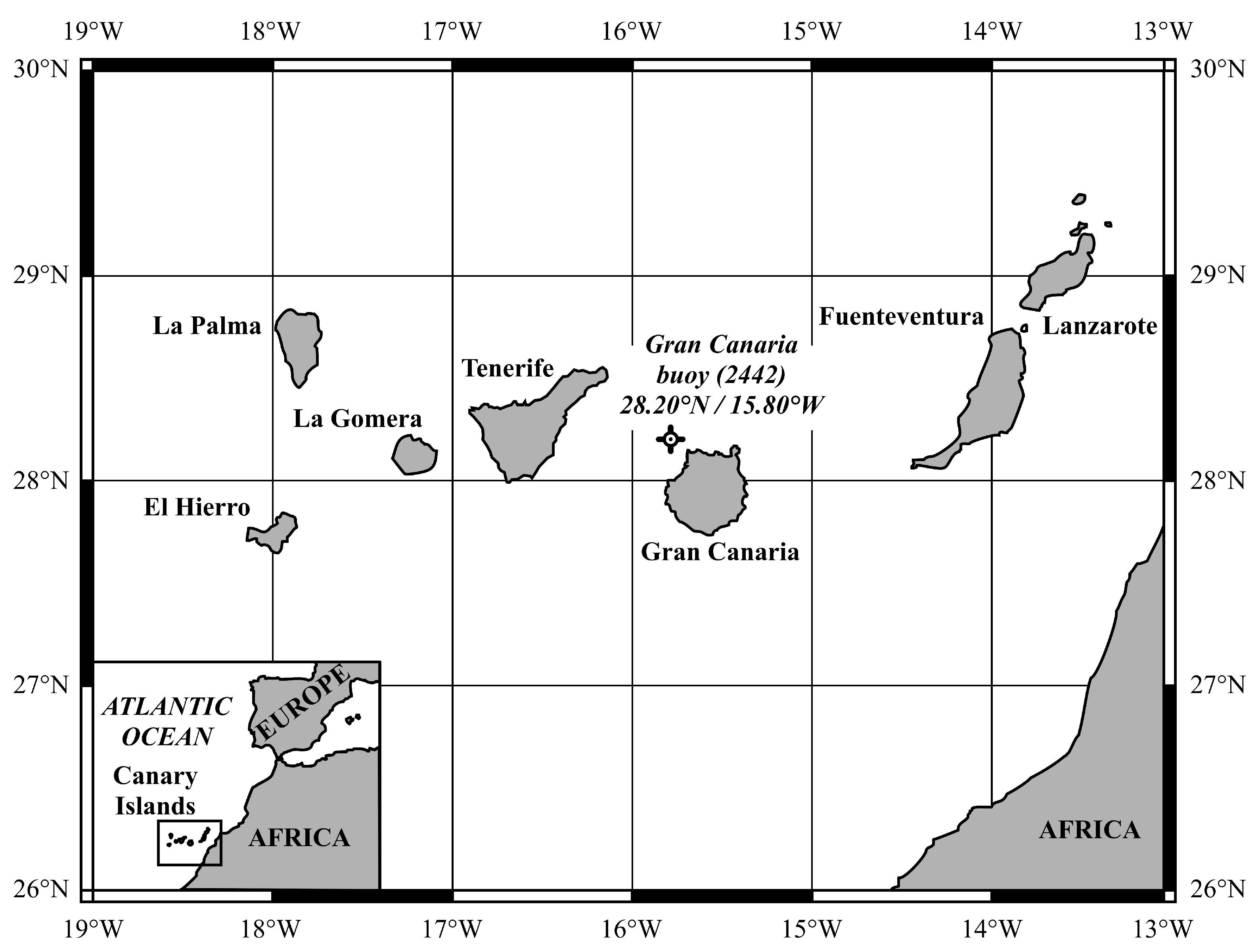
2. Data Sources
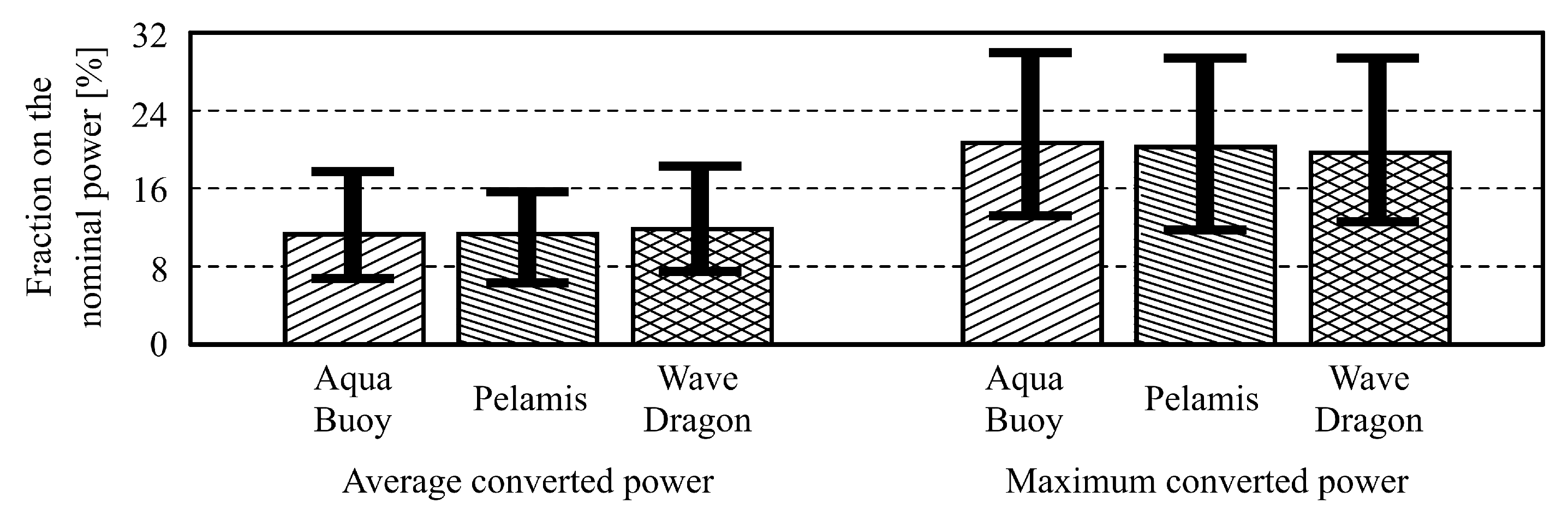
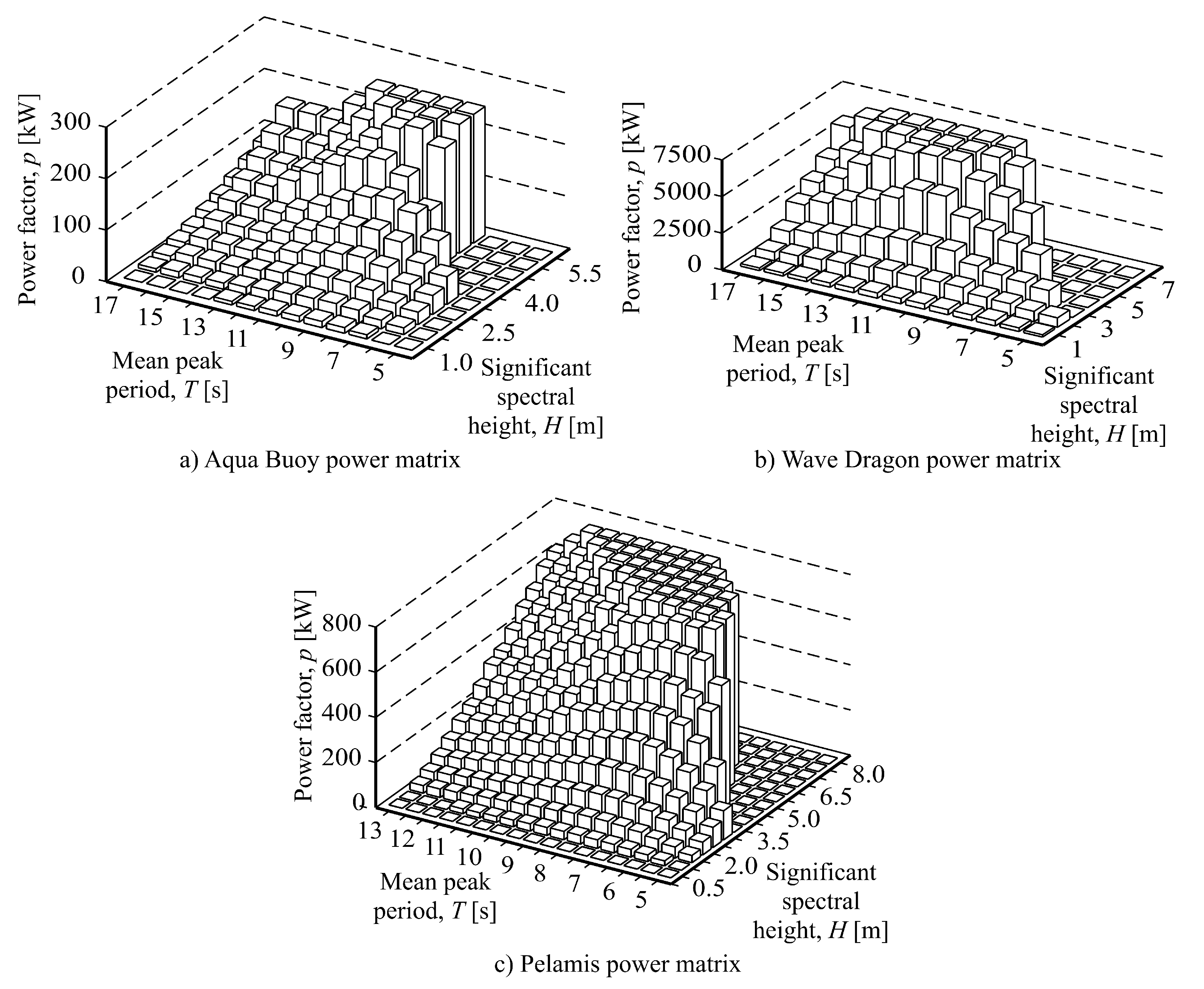
3. WECs Analyzed
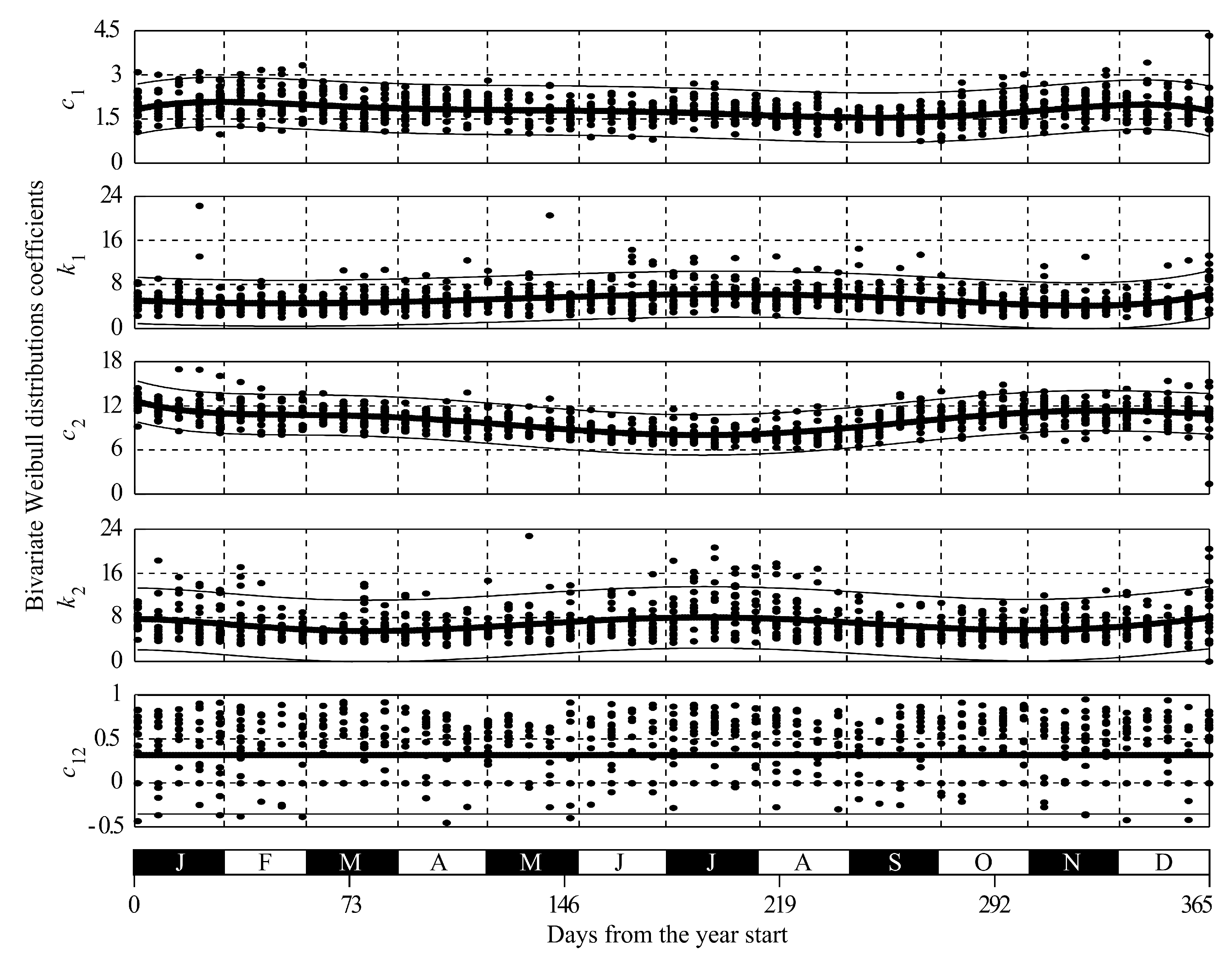
4. Bivariate Weibull Distribution Fitting
5. Bivariate Weibull Coefficient Models
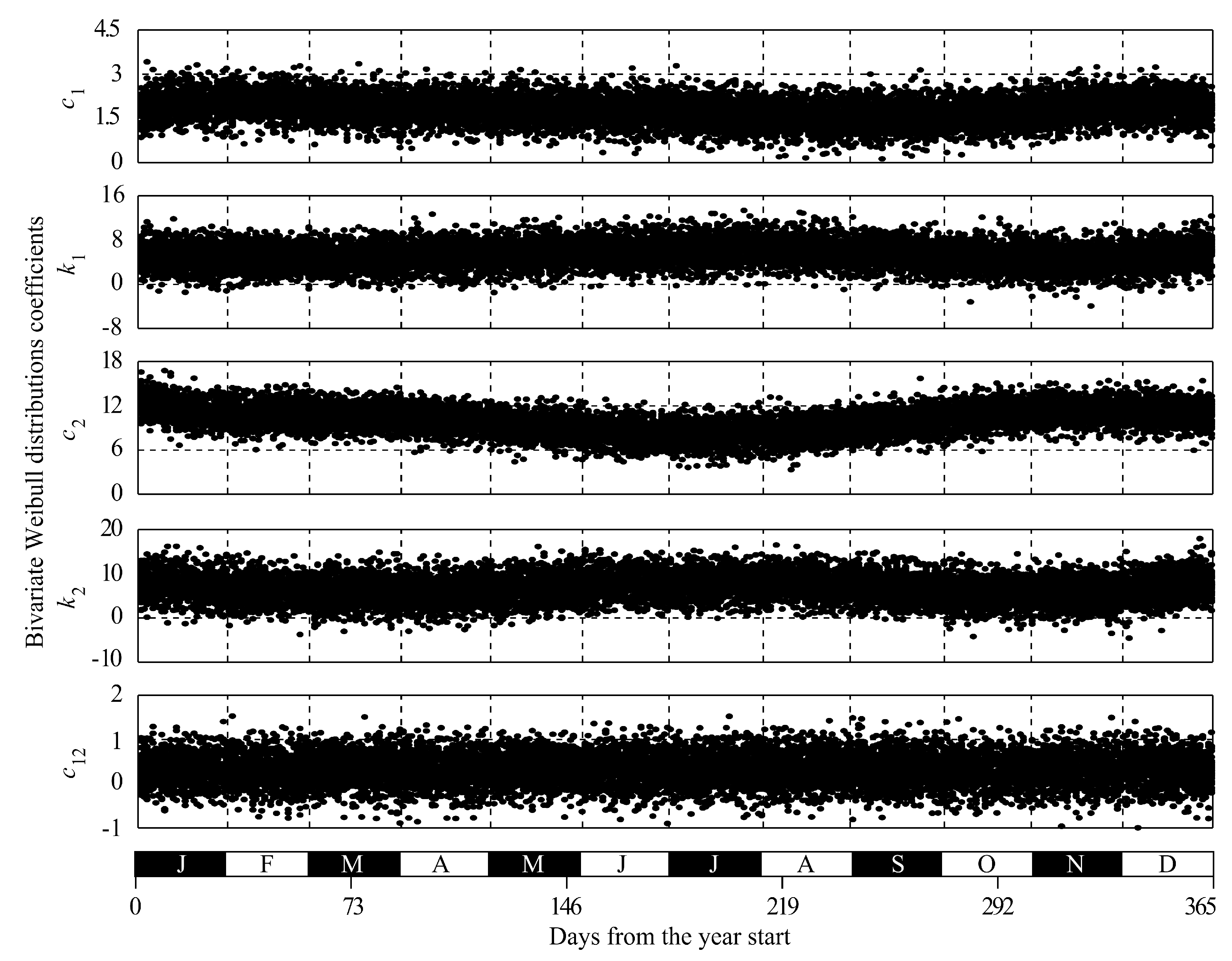
6. Monte Carlo Simulation of the Power Conversion
6.1. Random Values Generation
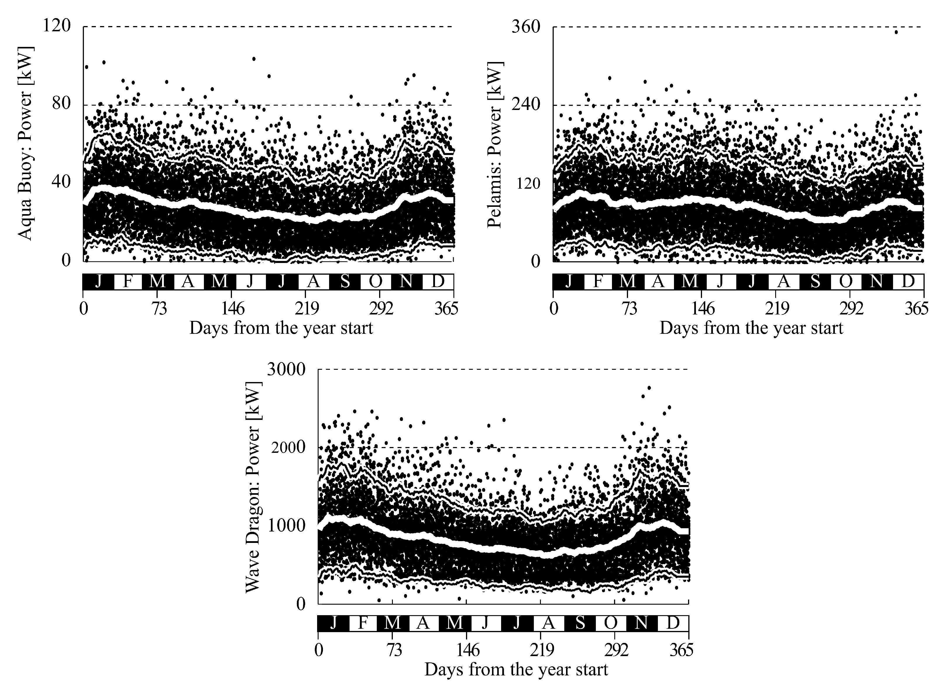
6.2. Power Conversion Computing
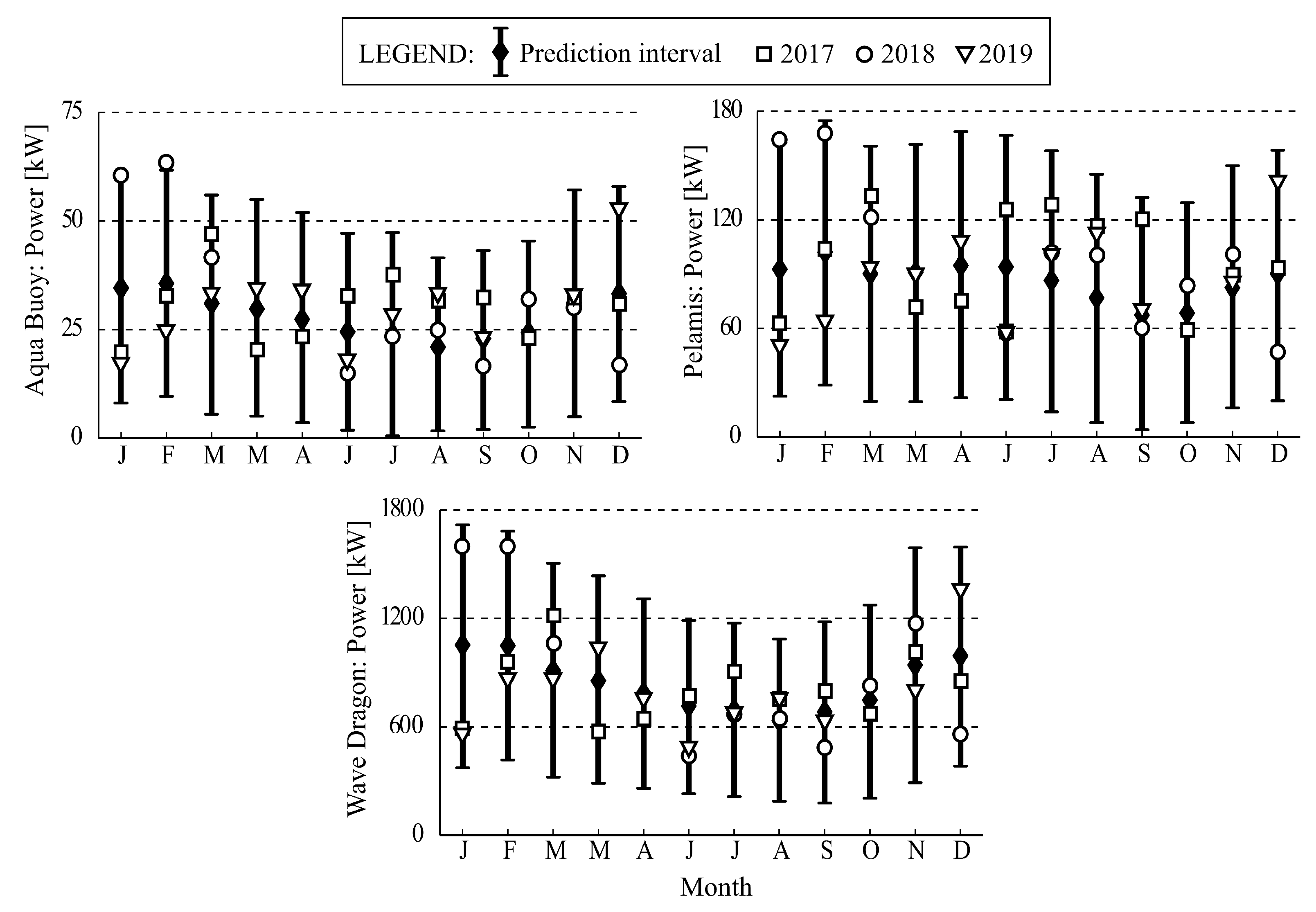
7. Validation
8. Conclusions
Author Contributions
Funding
Institutional Review Board Statement
Informed Consent Statement
Data Availability Statement
Acknowledgments
Conflicts of Interest
Appendix A. General Modeling Procedure
Appendix B. Regression Models Equations
Appendix B.1. Regression Model for Coefficient c1
Appendix B.2. Regression Model for Coefficient k1
Appendix B.3. Regression Model for Coefficient c2
Appendix B.4. Regression Model for Coefficient k2
Appendix B.5. Regression Model for Coefficient c12
References
- Fernández, J.M. Spain in the European Union. 2016. Available online: http://www.cvce.eu/obj/spain_in_the_european_union-en-7d6933cb-1a23-468c-bb15-93c2cf18c91f.html (accessed on 6 July 2020).
- European Commission. The Outermost Regions of the European Union: Towards a Partnership for Smart, Sustainable and Inclusive Growth. 2012. Available online: https://eur-lex.europa.eu/LexUriServ/LexUriServ.do?uri=COM%3A2012%3A0287%3AFIN%3AEN%3Apdf (accessed on 6 July 2020).
- Schallenberg, J.; Veza, J.M.; Blanco-Marigorta, A. Energy efficiency and desalination in the Canary Islands. Renew. Sustain. Energy Rev. 2014, 40, 741–748. [Google Scholar] [CrossRef]
- Gils, H.C.; Simon, S. Carbon neutral archipelago-100% renewable energy supply for the Canary Islands. Appl. Energy 2017, 188, 342–355. [Google Scholar] [CrossRef] [Green Version]
- González, A.; Pérez, J.C.; Díaz, J.; Expósito, F. Future projections of wind resource in a mountainous archipelago, Canary Islands. Renew. Energy 2017, 104, 120–128. [Google Scholar] [CrossRef] [Green Version]
- Ávila, D.; Marichal, G.N.; Padrón, I.; Quiza, R.; Hernández, A. Forecasting of wave energy in Canary Islands based on artificial intelligence. Appl. Ocean Res. 2020, 101, 102–189. [Google Scholar] [CrossRef]
- Sundseth, K. Natura 2000 in the Macaronesian Region. European Communities, 2009. Available online: https://ec.europa.eu/environment/nature/info/pubs/docs/biogeos/Macaronesian.pdf (accessed on 25 August 2021).
- Cropper, T.E.; Hanna, E. An analysis of the climate of Macaronesia, 1865–2012. Int. J. Climatol. 2014, 34, 604–622. [Google Scholar] [CrossRef] [Green Version]
- Meco, J.; Koppers, A.A.; Miggins, D.P.; Lomoschitz, A.; Betancort, J.F. The Canary record of the evolution of the North Atlantic Pliocene: New 40Ar/39Ar ages and some notable palaeontological evidence. Palaeogeogr. Palaeoclimatol. Palaeoecol. 2015, 435, 53–69. [Google Scholar] [CrossRef] [Green Version]
- Padrón, I.; Ávila, D.; Marichal, G.N.; Rodríguez, J.A. Assessment of hybrid renewable energy systems to supplied energy to autonomous desalination systems in two islands of the Canary Archipelago. Renew. Sustain. Energy Rev. 2019, 101, 221–230. [Google Scholar] [CrossRef]
- Fontán-Bouzas, Á.; Alcántara-Carrió, J.; Albarracín, S.; Baptista, P.; Silva, P.A.; Portz, L.; Manzolli, R.P. Multiannual shore morphodynamics of a cuspate foreland: Maspalomas (Gran Canaria, Canary Islands). J. Mar. Sci. Eng. 2019, 7, 416. [Google Scholar] [CrossRef] [Green Version]
- ISTAC (Canarian Statistic Institute). 2020. Available online: https://www.statcan.gc.ca/eng/start (accessed on 15 July 2020).
- Electrical Network of Spain. The Importance of a Connected Electrical Energy [El Valor de una Energía Conectada]. 2016. Available online: https://www.ree.es/sites/default/files/downloadable/diptico_canarias_2016_esp.pdf (accessed on 15 July 2020).
- Frydrychowicz-Jastrzebska, G. El Hierro renewable energy hybrid system: A tough compromise. Energies 2018, 11, 2812. [Google Scholar] [CrossRef] [Green Version]
- Gonçalves, M.; Martinho, P.; Guedes, C. Assessment of wave energy in the Canary Islands. Renew. Energy 2014, 68, 774–784. [Google Scholar] [CrossRef]
- Fernández Prieto, L.; Rodríguez Rodríguez, G.; Schallenberg Rodríguez, J. Wave energy to power a desalination plant in the north of Gran Canaria Island: Wave resource, socioeconomic and environmental assessment. J. Environ. Manag. 2019, 231, 546–551. [Google Scholar] [CrossRef] [PubMed]
- Iglesias, G.; Carballo, R. Wave resource in El Hierro: An island towards energy self-sufficiency. Renew. Energy 2011, 36, 689–698. [Google Scholar] [CrossRef]
- Lavidas, G.; Venugopal, V.; Friedrich, D. Wave energy extraction in Scotland through an improved nearshore wave atlas. Int. J. Mar. Energy 2017, 17, 64–83. [Google Scholar] [CrossRef] [Green Version]
- IDAE [Institute for the Diversification and Saving of Energy]. Wave Energy Evaluation. Technical Study. PER 2011–2020. 2011. Available online: https://www.idae.es/uploads/documentos/documentos_11227_e13_olas_b31fcafb.pdf (accessed on 10 June 2020).
- Falcão, A.F.O. Wave energy utilization: A review of the technologies. Renew. Sustain. Energy Rev. 2010, 14, 899–918. [Google Scholar] [CrossRef]
- Rusu, E.; Guedes Soares, C. Wave energy pattern around the Madeira Islands. Energy 2012, 45, 771–785. [Google Scholar] [CrossRef]
- Song, R.; Zhang, M.; Qian, X.; Wang, X.; Dai, Y.M.; Chen, J. A floating ocean energy conversion device and numerical study on buoy shape and performance. J. Mar. Sci. Eng. 2016, 4, 35. [Google Scholar] [CrossRef] [Green Version]
- Harnois, V.; Thies, P.R.; Johanning, L. On peak mooring loads and the influence of environmental conditions for marine energy converters. J. Mar. Sci. Eng. 2016, 4, 29. [Google Scholar] [CrossRef] [Green Version]
- O’Hagan, A.; Huertas, C.; O’Callaghan, J.; Greaves, D. Wave energy in Europe: Views on experiences and progress to date. Int. J. Mar. Energy 2016, 14, 180–197. [Google Scholar] [CrossRef] [Green Version]
- European Commission. Study on Lessons for Ocean Energy Development: Final Report; Publications Office of the European Union, Luxembourg: 2017. Available online: https://op.europa.eu/en/publication-detail/-/publication/03c9b48d-66af-11e7-b2f2-01aa75ed71a1 (accessed on 15 July 2020).
- EREC [European Renewable Energy Council]. Mapping Renewable Energy Pathways towards 2020: EU Roadmap. 2011. Available online: http://www.eufores.org/fileadmin/eufores/Projects/REPAP_2020/EREC-roadmap-V4.pdf (accessed on 16 July 2020).
- European Commission. Blue Energy Action Needed to Deliver on the Potential of Ocean Energy in European Seas and Oceans by 2020 and Beyond. 2014. Available online: https://eur-lex.europa.eu/legal-content/EN/TXT/?uri=CELEX%3A52014DC0008 (accessed on 18 July 2020).
- Trueworthy, A.; DuPont, B. The wave energy converter design process: Methods applied in industry and shortcomings of current practices. J. Mar. Sci. Eng. 2020, 8, 932. [Google Scholar] [CrossRef]
- Stratigaki, V. WECANet: The first open Pan-European network for marine renewable energy with a focus on wave energy-COST action CA17105. Water 2019, 11, 1249. [Google Scholar] [CrossRef] [Green Version]
- Barstow, S.; Mørk, G.; Mollison, D.; Cruz, J. The wave energy resource. In Ocean Wave Energy: Current Status and Future Perspectives; Cruz, J., Ed.; Springer: Berlin/Heidelberg, Germany, 2008; pp. 93–132. [Google Scholar]
- Puscasu, R. Integration of artificial neural networks into operational ocean wave prediction models for fast and accurate emulation of exact nonlinear interactions. Procedia Comput. Sci. 2014, 29, 1156–1170. [Google Scholar] [CrossRef] [Green Version]
- The Wamdi Group. The WAM model: A third generation ocean wave prediction model. J. Phys. Oceanogr. 1988, 18, 1775–1810. [Google Scholar] [CrossRef] [Green Version]
- SWAN Team. SWAN Scientific and Technical Documentation. 2020. Available online: http://swanmodel.sourceforge.net/download/zip/swantech.pdf (accessed on 3 September 2020).
- Malekmohamadi, I.; Bazargan-Lari, M.R.; Kerachian, R.; Nikoo, M.R.; Fallahnia, M. Evaluating the efficacy of SVMs, BNs, ANNs and ANFIS in wave height prediction. Ocean Eng. 2011, 38, 487–497. [Google Scholar] [CrossRef]
- Molina, O.; Castro, F.; Harrison, R.L. Efficiency assessments for different WEC types in the Canary Islands. In Developments in Maritime Transportation and Exploitation of Sea Resources; Soares, G., Peña, L., Eds.; Taylor and Francis Group: London, UK, 2014; pp. 879–887. [Google Scholar]
- Babarit, A.; Hals, J.; Muliawan, M.; Kurniawan, A.; Moan, T.; Krokstad, J. Numerical benchmarking study of a selection of wave energy converters. Renew. Energy 2012, 41, 44–63. [Google Scholar] [CrossRef]
- Raychaudhuri, S. Introduction to Monte Carlo simulation. In Proceedings of the 40th Conference on Winter Simulation, Miami Florida, 7–10 December 2008; pp. 91–100. [Google Scholar]
- Urquizo, J.; Calderón, C.; James, P. Using a local framework combining principal component regression and Monte Carlo simulation for uncertainty and sensitivity analysis of a domestic energy model in sub-city areas. Energies 2017, 10, 1986. [Google Scholar] [CrossRef] [Green Version]
- Kryzia, D.; Kuta, M.; Matuszewska, D.; Olczak, P. Analysis of the potential for gas micro-cogeneration development in Poland using the Monte Carlo method. Energies 2020, 13, 3140. [Google Scholar] [CrossRef]
- Da Silva Pereira, E.D.; Tavares Pinho, J.; Barros Galhardo, M.A.; Negrão Macêdo, W. Methodology of risk analysis by Monte Carlo method applied to power generation with renewable energy. Renew. Energy 2014, 69, 347–355. [Google Scholar] [CrossRef]
- Caralis, G.; Diakoulaki, D.; Yang, P.; Gao, Z.; Zervos, A.; Rados, K. Profitability of wind energy investments in China using a Monte Carlo approach for the treatment of uncertainties. Renew. Sustain. Energy Rev. 2014, 40, 224–236. [Google Scholar] [CrossRef]
- López-Ruiz, A.; Bergillos, R.J.; Ortega-Sánchez, M. The importance of wave climate forecasting on the decision-making process for nearshore wave energy exploitation. Appl. Energy 2016, 182, 191–203. [Google Scholar] [CrossRef]
- Hrafnkelsson, B.; Oddsson, G.; Unnthorsson, R. A method for estimating annual energy production using Monte Carlo wind speed simulation. Energies 2016, 9, 286. [Google Scholar] [CrossRef] [Green Version]
- Martinez-Velasco, J.A.; Guerra, G. Analysis of distribution systems with photovoltaic generation using a power flow simulator and a parallel Monte Carlo approach. Energies 2016, 9, 537. [Google Scholar] [CrossRef] [Green Version]
- Hiles, C.E.; Beatty, S.J.; De Andres, A. Wave energy converter annual energy production uncertainty using simulations. J. Mar. Sci. Eng. 2016, 4, 53. [Google Scholar] [CrossRef] [Green Version]
- Amirinia, G.; Kamranzad, B.; Mafi, S. Wind and wave energy potential in southern Caspian Sea using uncertainty analysis. Energy 2017, 120, 332–345. [Google Scholar] [CrossRef]
- Liu, W.; Guo, D.; Xu, Y.; Cheng, R.; Wang, Z.; Li, Y. Reliability assessment of power systems with photovoltaic power stations based on intelligent state space reduction and pseudo-sequential Monte Carlo simulation. Energies 2018, 11, 1431. [Google Scholar] [CrossRef] [Green Version]
- Wu, G.; Liu, C.; Liang, Y. Comparative study on numerical calculation of 2-d random sea surface based on fractal method and Monte Carlo method. Water 2020, 12, 1871. [Google Scholar] [CrossRef]
- Younesian, D.; Alam, M.R. Multi-stable mechanisms for high-efficiency and broadband ocean wave energy harvesting. Appl. Energy 2017, 197, 292–302. [Google Scholar] [CrossRef]
- Naess, A.; Gaidai, O.; Teigen, P. Extreme response prediction for nonlinear floating offshore structures by Monte Carlo simulation. Appl. Ocean Res. 2007, 29, 221–230. [Google Scholar] [CrossRef]
- Naess, A.; Gaidai, O.; Haver, S. Efficient estimation of extreme response of drag-dominated offshore structures by Monte Carlo simulation. Ocean Eng. 2007, 34, 2188–2197. [Google Scholar] [CrossRef]
- Bang, A.; Vanem, E.; Natvig, B. A new approach to environmental contours for ocean engineering applications based on direct Monte Carlo simulations. Ocean Eng. 2013, 60, 124–135. [Google Scholar] [CrossRef]
- Lin, W.; Su, C. An efficient Monte-Carlo simulation for the dynamic reliability analysis of jacket platforms subjected to random wave load. J. Mar. Sci. Eng. 2021, 9, 380. [Google Scholar] [CrossRef]
- Levent, M.; Elmar, C. Reliability analysis of a rubble mound breakwater using the theory of fuzzy random variables. Appl. Ocean Res. 2012, 39, 83–88. [Google Scholar] [CrossRef]
- Chian, C.Y.; Zhao, Y.Q.; Lin, T.Y.; Nelson, B.; Huang, H.H. Comparative study of time-domain fatigue assessments for an offshore wind turbine jacket substructure by using conventional grid-based and Monte Carlo sampling methods. Energies 2018, 11, 3112. [Google Scholar] [CrossRef] [Green Version]
- Rinaldi, G.; Thies, P.; Walker, R.; Johanning, L. On the analysis of a wave energy farm with focus on maintenance operations. J. Mar. Sci. Eng. 2016, 4, 51. [Google Scholar] [CrossRef] [Green Version]
- Kim, S.W.; Jang, H.K.; Cha, Y.J.; Yu, H.S.; Lee, S.J.; Yu, D.H.; Lee, A.R.; Jin, E.J. Development of a ship route decision-making algorithm based on a real number grid method. Appl. Ocean Res. 2020, 101, 102230. [Google Scholar] [CrossRef]
- Zhou, G.; Wang, Y.; Zhao, D.; Lin, J. Uncertainty analysis of ship model propulsion test on actual seas based on Monte Carlo method. J. Mar. Sci. Eng. 2020, 8, 398. [Google Scholar] [CrossRef]
- Faghih-Roohi, S.; Xie, M.; Ming, K. Accident risk assessment in marine transportation via Markov modelling and Markov Chain Monte Carlo simulation. Ocean Eng. 2014, 9, 363–370. [Google Scholar] [CrossRef]
- Kana, A.; Harrison, B. A Monte Carlo approach to the ship-centric Markov decision process for analyzing decisions over converting a containership to LNG power. Ocean Eng. 2017, 130, 40–48. [Google Scholar] [CrossRef] [Green Version]
- Kim, B.; Kim, T.W. Monte Carlo simulation for offshore transportation. Ocean Eng. 2017, 129, 177–190. [Google Scholar] [CrossRef]
- Salem, A. Use of Monte Carlo simulation to assess uncertainties in fire consequence calculation. Ocean Eng. 2016, 117, 411–430. [Google Scholar] [CrossRef]
- Harbors of State of Spain. Waves Average. Buoy of Gran Canaria 2442 [Clima Boya de Gran Canaria, 2442]. 2017. Available online: http://www.puertos.es/es-es/oceanografia/Paginas/portus_OLD.aspx (accessed on 8 June 2020).
- Clemente, D.; Rosa-Santos, P.; Taveira-Pinto, F. On the potential synergies and applications of wave energy converters: A review. Renew. Sustain. Energy Rev. 2021, 135, 110–162. [Google Scholar] [CrossRef]
- Ahamed, R.; McKee, K.; Howard, I. Advancements of wave energy converters based on power take off (PTO) systems: A review. Ocean Eng. 2020, 204, 107248. [Google Scholar] [CrossRef]
- Padrón, I.; Avila, D.; Marichal, G. Assessment of wave energy converters systems to supplied energy to desalination systems in the El Hierro Island. In Proceedings of the 3rd International Conference on Offshore Renewable Energy. (CORE 2018), Lisbon, Portugal, 8–10 October 2018. [Google Scholar]
- Astariz, S.; Iglesias, G. Selecting optimum locations for co-located wave and wind energy farms. Part I: The co-Location feasibility index. Energy Convers. Manag. 2016, 122, 589–598. [Google Scholar] [CrossRef] [Green Version]
- Astariz, S.; Iglesias, G. Selecting optimum locations for co-located wave and wind energy farms. Part II: A case study. Energy Convers. Manag. 2016, 122, 599–608. [Google Scholar] [CrossRef] [Green Version]
- Weinstein, A.; Fredrikson, G.; Parks, M.J.; Neislen, K. Aqua Buoy-The offshore wave energy converter: Numerical modeling and optimization. In Proceedings of the Oceans’04 MTS/IEEE Techno-Ocean’04, Kobe, Japan, 9–12 November 2004. [Google Scholar]
- Henderson, R. Design, simulation, and testing of a novel hydraulic power take-off system for the Pelamis wave energy converter. Renew. Energy 2006, 31, 271–283. [Google Scholar] [CrossRef]
- Kofoed, J.; Frigaard, P.; Friis-Madsen, E.; Sørensen, H. Prototype testing of the wave energy converter Wave Dragon. Renew. Energy 2006, 31, 181–189. [Google Scholar] [CrossRef] [Green Version]
- Silva, D.; Rusu, E.; Guedes, C. Evaluation of various technologies for wave energy conversion in the Portuguese nearshore. Energies 2013, 6, 1344–1364. [Google Scholar] [CrossRef]
- Sorensen, R. Basic Coastal Engineering; Springer: New York, NY, USA, 2006. [Google Scholar]
- Desouky, M.A.A.; Abdelkhalik, O. Wave prediction using wave rider position measurements and NARX network in wave energy conversion. Appl. Ocean Res. 2019, 82, 10–21. [Google Scholar] [CrossRef]
- Oh, S.H.; Suh, K.D.; Son, S.Y.; Lee, D.Y. Performance comparison of spectral wave models based on different governing equations including wave breaking. J. Civ. Eng. 2009, 13, 75–84. [Google Scholar] [CrossRef] [Green Version]
- Dominguez, J.C.; Cienfuegos, R.; Catalán, P.; Zamorano, L.; Lucero, F. Assessment of fast spectral wave transfer methodologies from deep to shallow waters in the framework of energy resource quantification in the Chilean coast. Coast. Eng. Proc. 2014, 34, 23. [Google Scholar] [CrossRef] [Green Version]
- Kiusalaas, J. Numerical Methods in Engineering with MATLAB; Cambridge University Press: Cambridge, UK, 2005. [Google Scholar]


| Model | MAE | |||
|---|---|---|---|---|
| 0.121 | 0.34 | ≈0 | ||
| 0.092 | 1.54 | ≈0 | ||
| 0.433 | 1.04 | ≈0 | ||
| 0.079 | 2.10 | |||
| ≈0 | 0.31 | ≈0 | ≈0 |
| i | ||
|---|---|---|
| 1 | 0.236927 | –0.906180 |
| 2 | 0.478629 | –0.538469 |
| 3 | 0.568889 | 0.000000 |
| 4 | 0.478629 | 0.538469 |
| 5 | 0.236927 | 0.906180 |
Publisher’s Note: MDPI stays neutral with regard to jurisdictional claims in published maps and institutional affiliations. |
© 2021 by the authors. Licensee MDPI, Basel, Switzerland. This article is an open access article distributed under the terms and conditions of the Creative Commons Attribution (CC BY) license (https://creativecommons.org/licenses/by/4.0/).
Share and Cite
Avila, D.; Marichal, G.N.; Quiza, R.; San Luis, F. Prediction of Wave Energy Transformation Capability in Isolated Islands by Using the Monte Carlo Method. J. Mar. Sci. Eng. 2021, 9, 980. https://doi.org/10.3390/jmse9090980
Avila D, Marichal GN, Quiza R, San Luis F. Prediction of Wave Energy Transformation Capability in Isolated Islands by Using the Monte Carlo Method. Journal of Marine Science and Engineering. 2021; 9(9):980. https://doi.org/10.3390/jmse9090980
Chicago/Turabian StyleAvila, Deivis, Graciliano Nicolás Marichal, Ramón Quiza, and Felipe San Luis. 2021. "Prediction of Wave Energy Transformation Capability in Isolated Islands by Using the Monte Carlo Method" Journal of Marine Science and Engineering 9, no. 9: 980. https://doi.org/10.3390/jmse9090980
APA StyleAvila, D., Marichal, G. N., Quiza, R., & San Luis, F. (2021). Prediction of Wave Energy Transformation Capability in Isolated Islands by Using the Monte Carlo Method. Journal of Marine Science and Engineering, 9(9), 980. https://doi.org/10.3390/jmse9090980