Application of Deep Reinforcement Learning to Predict Shaft Deformation Considering Hull Deformation of Medium-Sized Oil/Chemical Tanker

Abstract

The enlargement of ships has increased the relative hull deformation owing to draft changes. Moreover, design changes such as an increased propeller diameter and pitch changes have occurred to compensate for the reduction in the engine revolution and consequent ship speed. In terms of propulsion shaft alignment, as the load of the stern tube support bearing increases, an uneven load distribution occurs between the shaft support bearings, leading to stern accidents. To prevent such accidents and to ensure shaft system stability, a shaft system design technique is required in which the shaft deformation resulting from the hull deformation is considered. Based on the measurement data of a medium-sized oil/chemical tanker, this study presents a novel approach to predicting the shaft deformation following stern hull deformation through inverse analysis using deep reinforcement learning, as opposed to traditional prediction techniques. The main bearing reaction force, which was difficult to reflect in previous studies, was predicted with high accuracy by comparing it with the measured value, and reasonable shaft deformation could be derived according to the hull deformation. The deep reinforcement learning technique in this study is expected to be expandable for predicting the dynamic behavior of the shaft of an operating vessel.

1. Introduction

Since the 2000s, hull stiffness has been reduced owing to the enlargement of ships, which has been achieved along with the growth of the global economy. Moreover, significant hull deformation occurs as a result of to the relatively large loading changes in the aft peak tank (APT) and draft. As the stiffness of the shaft increases owing to the increased engine power, the hull deformation causes the reaction force of the bearings that support the shaft to be distributed more unevenly. Furthermore, the ultra-long stroke engine has recently been introduced for energy efficiency. Thus, as the propeller diameter increases and changes in pitch, the propeller weight increases to compensate for the decrease in the engine revolution caused by the long stroke and consequent ship speed, which further increases the stern load [1]. Owing to the above factors, the hull deformation causes shaft deformation, which results in accidents relating to heat generation of the stern tube bearings, abnormal wear, and damage in terms of the shaft alignment [2]. Such damage occurs as an excessive local load concentration on specific bearings, whereas the adjacent bearings form no load, resulting in an uneven distribution of each bearing load. Thus, it is necessary to ensure shaft system stability by performing shaft alignment with appropriate bearing load distribution considering the hull deformation [3,4,5,6].

Many studies have been conducted to evaluate the shaft stability considering the shaft deformation owing to hull deformation. Representative examples of such work include a study that predicted shaft deformation using the finite element method in the analysis of a model of the stern structure [7,8,9] and another study whose prediction of shaft deformation was demonstrated to sufficiently reflect measurements by applying the measured data to various inverse-analysis techniques. [3,10,11] Stern structural analysis has been performed using the finite element (FE) method, and in certain studies, inverse analysis of the measured data has been performed. Choung and Choe [7] generated FE models for shaft systems, double bottoms, and main engines to predict the hull deformation and shaft deformation. Korbetis et al. [8] performed global structural analysis with a finely modeled stern of a 320 K DWT VLCC and predicted the shaft deformation according to the loading conditions by applying the lumped weight of the main engine, without separate modeling of the shaft and engine. Moreover, Seo et al. [9] performed global structural analysis with a finely modeled stern of a 300 K DWT VLCC and predicted the shaft deformation according to the draft by modeling the shaft, engine, and engine foundation separately. However, in studies on stern structural analysis using the FE method, significant deviation of the main bearing (MB) reaction force occurred in the shaft deformation prediction according to the draft, and it was difficult to consider the actual ship conditions and load distribution of the engine room equipment.

Rao et al. [10] generated the reaction force influence number (RIN) matrix from the bearing reaction force that was calculated by the bending moment measured with a strain gauge and applied inverse analysis to predict the shaft deformation. Šverko [3] predicted the shaft deformation using a genetic algorithm from the bearing reaction force that was measured by the jack-up method and the bending moment that was measured by a strain gauge. Lee [11] predicted the shaft deformation using a trial-and-error method according to the bending moment that was measured with a strain gauge. However, the techniques used in this inverse-analysis study had the limitation of being unable to make predictions that sufficiently reflected measurements due to its sensitivity to shaft deformation, whereby a large reaction force is generated even with a minor deformation of the shaft.

Compared to stern structural analysis using the FE method, in the inverse analysis method using the measured data, the measured bearing reaction force and bending moment can be used to predict the shaft deformation, thereby reflecting the hull deformation that is caused by the actual draft conditions of the ship, the load distribution in the engine room, and the APT loading. However, it is also difficult to predict the shaft deformation considering the reaction force of the MBs. Therefore, it is necessary to develop a technique for the inverse analysis of shaft deformation that can sufficiently reflect the MB reaction force.

Recent advances in computing performance have contributed to active research using deep neural networks and reinforcement learning (RL) in various fields. The structure of the deep neural network mimics the human brain and neural network. This technique can perform complex nonlinear analysis that is difficult to achieve with an equation for variables without prior definition [12]. RL changes to the “next state” by selecting an “action” from the “state” based on the content learned through trial and error to obtain a “reward,” and an action or action pattern is selected that maximizes the sum of the rewards. Deep RL, which combines RL and deep neural networks, has been successfully applied to various problems, such as control, recommendation, optimization, and detection [13]. Uyanik et al. [14] predicted the fuel consumption of container ships using various machine learning techniques. Cheliotis et al. [15] detected abnormal symptoms of ships using machine learning. Kim et al. [16] predicted the fuel consumption rate of container ships using a deep neural network and presented the optimal operating conditions accordingly. Song et al. [17] conducted a study on the detection of ships through synthetic aperture radar (SAR) images and automatic identification system (AIS) information using a convolutional neural network. Karvelis et al. [18] studied structural health monitoring by attaching a sensor to the hull structure and using an autoencoder. Scardua et al. [19] proposed optimal ship unloader control by applying an artificial neural network to RL. Fu et al. [20] investigated the detection of the rotation of a berthing ship using RL. Zhao and Rho [21] conducted a study on the collision avoidance of ships according to COLREG using deep RL. As described above, various studies have been carried out on the successful application of deep neural networks and deep RL to ships. However, no research to date has applied deep RL to the shaft system of a ship, and it is expected that the use of deep RL in the inverse analysis of the measured data will be suitable for the shaft deformation problem.

In this study, measured values of the shaft under various draft conditions were applied as input variables to the deep-RL-based algorithm, with the output being the prediction of shaft deformation features that sufficiently reflect measured values. First, the supporting bearing reaction force of the shaft system and the shaft bending moment of the target ship were measured according to the draft. This was followed by creating an FE model of the shaft system of the target ship to check the fit of the measured and calculated values. Thereafter, a deep RL algorithm was modeled for use in inverse analysis, and the shaft deformation was predicted through an inverse analysis algorithm by applying deep RL using the measured values. Subsequently, the trends in the predicted shaft deformation were identified and substituted into the shaft model to evaluate how effectively the measured values could be reflected. Finally, the results were compared with those of shaft deformation prediction using existing research techniques. The purpose of this study was to determine the academic significance of the shaft deformation prediction of inverse analysis by applying deep RL.

2. Materials and Methods

Figure 1 presents the research procedure of this study.

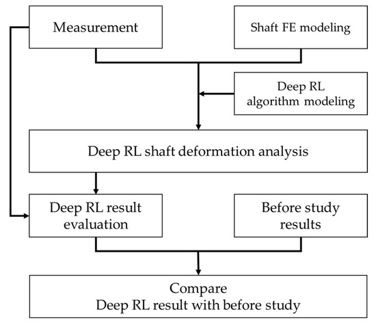
Figure 1. Outline of study.

2.1. Target Ship Specifications

The target ship of this study was a 50,000 DWT medium-sized oil/chemical tanker that was equipped with a highly energy-efficient long-stroke engine. The specifications of target ship are presented in Table 1 and the specifications of the shaft system of the target ship are listed in Table 2.

Table 1. Specifications of target ship.

Description	Value
GT [ton]	29,327
SDWT [ton]	49,635
Length OA [m]	183.1
Length BP [m]	174.0
Breadth MLD [m]	32.2
Depth MLD [m]	19.1
Draft design MLD [m]	11.0
Draft scantling MLD [m]	13.2
Year built	2015

Table 2. Specifications of shaft system of target ship.

Category	Description	Value
Main engine	Type	MAN B&W 6G50ME-B
	MCR	7700 kW × 93.4 rpm
	NCR	5344 kW × 82.7 rpm
Propeller	No. of blades	4-blade fixed pitch
	Diameter	6600 mm
	Material	Ni-Al-bronze
	Mass in air	18,200 kg
	Cap & nut mass	1538 kg
Flywheel	Mass	11,207 kg

2.2. Shaft System Measurement Methods

2.2.1. Bearing Reaction Force Measurement Using Jack-Up Method

As illustrated in Figure 2, the forward stern tube bearings were omitted in the propulsion shaft system of the target ship. The aft stern tube bearing (ASTB), intermediate bearing (IB), and eight MBs were aligned with the main engine crank, which was installed linearly.

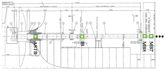
Figure 2. Bearing positions of target ship.

Typical methods for measuring the shaft reaction force include the jack-up method, which measures the bearing reaction force directly using a hydraulic jack, and the strain gauge method, which calculates the reaction force by obtaining the bending moment from the strain that is measured by attaching a strain gauge to the shaft and applying the moment equilibrium equation. In the jack-up method, the reaction force of the bearing is measured directly by installing a hydraulic jack near the bearing position, as indicated in Figure 3. The reaction force of the IB is measured by installing a hydraulic jack on the foundation, as illustrated in Figure 3a. The reaction force of the MBs excluding the aftmost MB is determined by turning the crank arm to a horizontal position in the direction of the exhaust pipe, as indicated in Figure 3b, following which measurement is performed by installing a hydraulic jack on the crank arm that is adjacent to the measured bearing. The reaction force of the aftmost MB is measured by installing a rigid steel beam under the hydraulic jack and a steel bar between the flywheel and hydraulic jack, as illustrated in Figure 3c. However, as the stern tube bearing is located in the stern tube, making it difficult to access, it is impossible to install a hydraulic jack at the bearing position.

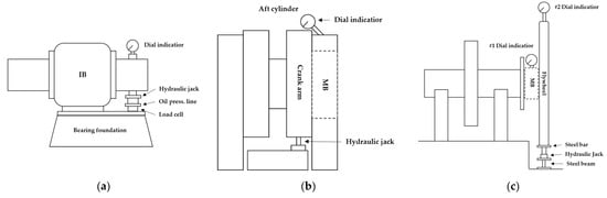
Figure 3. Measurement using jack-up method: (a) intermediate bearing (IB), (b) main bearings (MBs) excluding aftmost MB, and (c) aftmost MB.

The advantages of the jack-up method are that it is simple, and measurement can be performed using only a hydraulic jack and a dial indicator. Furthermore, it is the only method in which the reaction force is measured directly. However, the disadvantages are that it is not possible to measure the bearing reaction force against the rotating shaft, it is not possible to measure the bearing reaction force against the shaft during a ship voyage, the same hydraulic jack must be used for repeated measurements, and the measured value may exhibit errors depending on the installation degree [22].

2.2.2. Bending Moment Measurement Using Strain Gauge

The strain gauge method provides the moment and reaction force for the shaft system alignment using the flexural beam theory. The Wheatstone bridge circuit connection used in the strain gauge method is divided into one gauge (quarter gauge), two gauges (half gauge), and four gauges (full gauge) according to the number of attached gauges. In this study, the two-gauge method was used in consideration of the utility versus installation time. The strain gauge used was the WFLA-3-11-L1 manufactured by TML (Tokyo Sokki Kenkyujo). As illustrated in Figure 4a,c,d the two gauges, spaced 180 degrees above and below the shaft surface, were attached with a Wheatstone bridge connection, as indicated in Figure 4b. The resistance value of the strain gauge changes proportionally to the vertical strain of the shaft that is caused by the rotation of the shaft, and in this manner, a variable output voltage compared to the input voltage can be obtained. The strain in the strain gauge can be determined from the initial resistance and the amount of change in the resistance using Equation (1).

$$ϵ=\frac{\mathsf{\Delta }R}{R}\cdot \frac{1}{k}$$

(1)

where $ϵ$ is the strain, $R$ is the initial resistance measured by the strain gauge, $\mathsf{\Delta }R$ is the amount of change in the resistance measured by the strain gauge, and $k$ is the strain gauge coefficient.

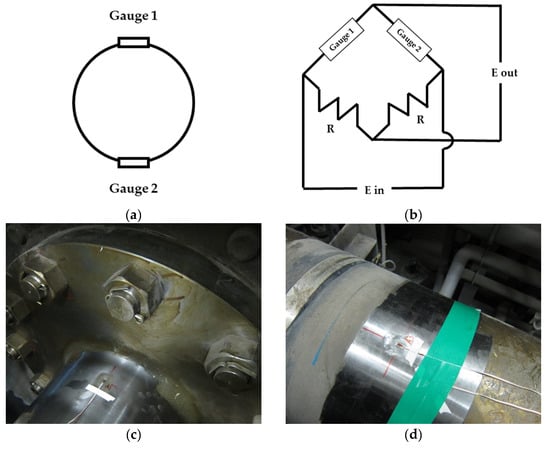
Figure 4. (a) Wheatstone bridge connection method, (b) strain gauge attachment locations, and (c,d) strain gauge attachment examples.

According to the strain obtained in Equations (1) and (2) is used to calculate the bending stress in the two-gauge method, as illustrated in Figure 4a,b.

$${\sigma }_b=\frac{1}{2}E\left({ϵ}_b-{ϵ}_t\right),$$

(2)

where ${\sigma }_b$ is the bending stress, ${ϵ}_b$ is the strain amplitude of the strain gauge that is installed in the lower part, ${ϵ}_t$ is the strain amplitude of the strain gauge that is installed in the lower part, and $E$ is the Young’s modulus.

According to the bending stress obtained in Equation (2), the bending moment is obtained from the relational equation for the beam theory, as per Equation (3):

$$M_b={\sigma }_b\frac{\pi \left(D_o^4-D_i^4\right)}{32D_0} ,$$

(3)

where $M_b$ is the bending moment, $D_o$ is the outer diameter of the shaft, and $D_i$ is the inner diameter of the shaft.

The advantage of the strain gauge method is that the reaction force is calculated using the moment equilibrium equation. Thus, the reaction force of the stern tube bearing that is located at the end of the stern tube can be calculated and the reaction force can be measured while the shaft is rotating during the ship voyage. However, the disadvantage is that, in the case of the MB, it is impossible to install the gauge inside the engine. Therefore, the reaction force cannot be calculated, the installation time is long, and the equipment is sensitive and expensive [22].

2.2.3. Measurement Results

Table 3 displays the fore and aft drafts under the measured draft conditions for the reaction force and bending moment of the target ship, whereas Figure 5 depicts the stern drafts under the measured draft conditions of the target ship. D1 (Figure 5a) denotes a light condition with no cargo loaded, D2 (Figure 5b) is an empty APT in the ballast condition, and D3 (Figure 5c) is a full APT in the ballast condition. D4 (Figure 5d) is an empty APT in the scantling condition and D5 (Figure 5e) is a full APT in the scantling condition. The reaction force of the shaft support bearings and bending moment of the strain gauges were measured under the above five draft conditions.

Table 3. Fore and aft drafts under measurement draft conditions.

Draft Condition	Description	Fore Draft [m]	Aft Draft [m]
D1	Light ballast APT empty	3.40	6.60
D2	Ballast APT empty	6.30	7.90
D3	Ballast APT full	6.45	8.95
D4	Scantling APT empty	13.50	12.50
D5	Scantling APT full	13.20	12.60

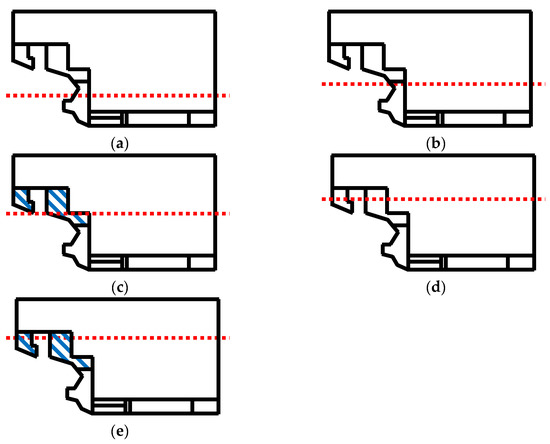
Figure 5. Stern draft according to measurement draft conditions: (a) D1, (b) D2, (c) D3, (d) D4, and (e) D5.

The reaction force of the target vessel could be measured using the jack-up method with a hydraulic jack by stopping the engine under the conditions displayed in Table 3 and performing the measurement. Table 4 lists the reaction force measurement results of the IB and the MBs measured under each draft condition.

Table 4. Jack-up measurement results.

	D1 [kN]	D2 [kN]	D3 [kN]	D4 [kN]	D5 [kN]
IB	70.3	71.4	65.5	69.9	67.2
MB8	9.9	18.7	32.9	77.7	93.1
MB7	178.6	132.5	153.8	126.2	103.5
MB6	109.6	96.0	102.6	78.0	97.7

In this study, strain gauges were installed at seven positions, as illustrated in Figure 6, the exact positions of which are detailed in Table 5. The strain was measured by rotating the shaft from one to two turns at a low speed of 2–5 rpm using a turning gear. Table 6 presents the bending moment measurement results of the measured strain gauges.

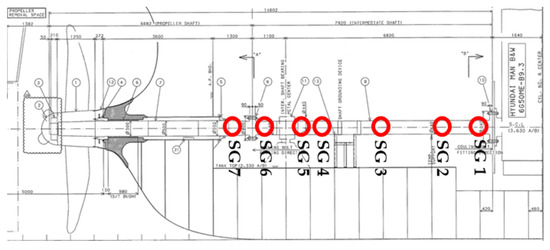
Figure 6. Strain gauge attachment locations.

Table 5. Detailed strain gauge attachment locations.

Strain Gauges	Distance from Shaft End [mm]
SG7	5862
SG6	6875
SG5	8137
SG4	8972
SG3	10,467
SG2	12,712
SG1	14,422

Table 6. Strain gauge measurement results.

	D1 [kNm]	D2 [kNm]	D3 [kNm]	D4 [kNm]	D5 [kNm]
SG7	85.1	75.1	64.6	83.8	73.3
SG6	77.4	67.3	61.0	82.8	74.4
SG5	59.3	52.3	44.1	69.2	63.2
SG4	12.5	−7.5	2.9	30.5	24.3
SG3	−58.1	−55.6	−56.0	−23.4	−28.0
SG2	−107.5	−100.4	−93.2	−54.8	−59.0
SG1	−109.6	−99.9	−86.1	−40.6	−42.2

The reaction force of the ASTB could not be measured by installing a hydraulic jack. Thus, the reaction force of the ASTB ($R_{\mathrm{ASTB}}$), effective support point of the ASTB ($B$), no. 7 strain gauge attachment position ($A$), and propeller weight ($W_p$) were simply expressed as shown in Figure 7. On this basis, the moment equilibrium equation in Equation (4) was established, and an equation for the ASTB reaction force was established as in Equation (5).

$$\begin{gathered} {{\displaystyle \sum }}^{ }{M}_A=M_A-R_{ASTB}{d}_1+W_p{d}_2+M_{AB}=0 \\ \left(where M_{AB}=W_{AB}\frac{d_1}{2}\right) \end{gathered}$$

(4)

$$R_{ASTB}=\frac{1}{d_1}\left\{M_A+M_{AB}+W_p{d}_2\right\},$$

(5)

where $M_A$ is the bending moment measured at the no. 7 strain gauge, $R_{\mathrm{ASTB}}$ is the reaction force of the ASTB, $d_1$ is the distance from the effective support point of the ASTB ($B$) to the attachment position of the no. 7 strain gauge ($A$), $W_p$ is the load of the propeller, $d_2$ is the distance from the support point of the propeller to the attachment position of the no. 7 strain gauge ($A$), and $M_{AB} \mathrm{and} W_{AB}$ are the bending moment and weight of the shaft from the effective support point of the stern tube bearing to the attachment position of the no. 7 strain gauge ($A$), respectively.

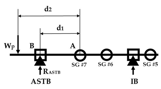
Figure 7. ASTB moment equilibrium equation.

Table 7 displays the results of the reaction force of the ASTB calculated under the draft conditions in Table 3.

Table 7. Calculation results of ASTB reaction force.

	D1 [kN]	D2 [kN]	D3 [kN]	D4 [kN]	D5 [kN]
ASTB (calculated)	253.26	250.53	247.67	252.91	250.04

2.3. Deep RL

2.3.1. Deep Neural Network

As illustrated in Figure 8, the deep neural network consists of an input layer that receives input variables, a hidden layer that receives variables from the input layer and performs calculations, and an output layer that receives the results from the hidden layer and outputs them. Such a network is known as an artificial neural network because weights and biases are applied as per Equation (6) as it progresses from a node constituting a layer to a node in the next layer, and it is transmitted to the next layer through an activation function inside the hidden layer. An artificial neural network in which many layers are stacked is referred to as a deep neural network [23].

$$\left[i_1, i_2\right]\times \left[\begin{array}{cc}{w}_{h11}& w_{h12}\\ w_{h21}& w_{h22}\end{array}\right]+\left[b_{h1}, b_{h2}\right]=\left[H_1, H_2\right],$$

(6)

where $i_1 \mathrm{and} i_2$ are the nodes of the input layer; $w_{11}, w_{12}, w_{21}, \mathrm{and} w_{22}$ are the weights that are applied to the nodes when transmitting from the input layer to the hidden layer; $b_{h1} \mathrm{and} b_{h2}$ are the biases that are applied to the nodes; and $H_1 \mathrm{and} H_2$ are the values of the nodes of the hidden layer.

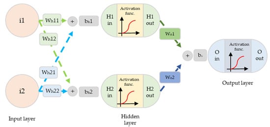
Figure 8. Schematic of artificial neural network.

In a deep neural network, the process of calculating all of the given data from the input layer to the output layer, as indicated in Figure 9, is known as the “epoch,” and the function representing the error between the target value and output value after the end of the epoch is referred to as a “loss function.” In deep neural network learning, this error is calculated in the opposite direction to that of the neural network to reduce the loss function, which is known as “back propagation.” As this process is performed repeatedly through the optimization technique, the weight and bias of the node are updated and a value that is close to the target value is output.

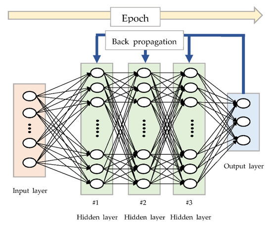
Figure 9. Schematic of deep neural network.

2.3.2. RL

RL is a technique that was developed based on the dynamic programming method proposed by Bellman [24]. It can be categorized as value-based RL and policy-based RL depending on whether an action or a policy is selected to maximize the value. Value-based RL was applied in this study because the purpose was to determine the optimal value, and not the policy to determine the optimal value.

Q-learning, which is a representative algorithm of value-based RL [25], performs an action ($a_t$) in the current state ($S_t$) of the $t^{th}$ episode, as indicated in Equation (7) and Figure 10. The value ($Q$) is updated through the weighted sum of the maximum value in the next state ($\underset{a_{t+1}}{\max }Q\left(S_{t+1},a_{t+1}\right)$) and the previous value ($Q\left(S_t,a_t\right)$) that is calculated by receiving rewards ($R_t$) according to the next state ($S_{t+1}$).

$$Q\left(S_t,a_t\right)\leftarrow Q\left(S_t,a_t\right)+\alpha \left[R_t+\gamma \underset{a_{t+1}}{\max }Q\left(S_{t+1},a_{t+1}\right)-Q\left(S_t,a_t\right)\right]$$

(7)

where $Q\left(S_t,a_t\right)$is the value when an action ($a_t$) is performed in a state ($S_t$), α is the learning rate indicating the update degree, $R_t$ is the reward, and $\gamma$ is the discount rate for the future reward. Furthermore, $\underset{a_{t+1}}{\max }Q\left(S_{t+1},a_{t+1}\right)$is the greatest value obtained when an action ($a_{t+1}$) is selected in the next state ($S_{t+1}$).

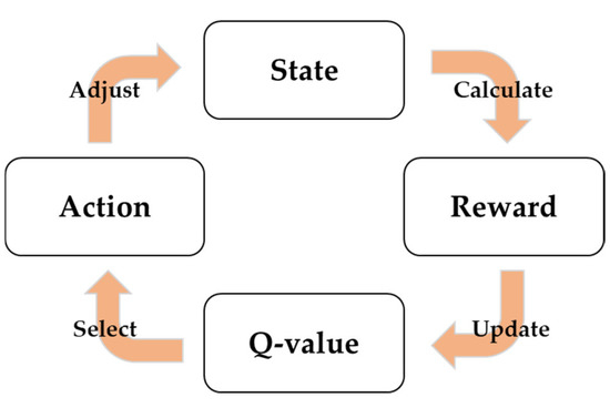
Figure 10. Schematic of Q-learning [26].

2.3.3. Deep RL

Deep RL uses a deep neural network to determine a behavior in RL and performs back propagation to reduce the loss function of the Q-value for the behavior. The deep Q-learning network is a method that combines Q-learning and deep neural networks [27]. This algorithm selects a random action with a probability of $ϵ$ as in Equation (8) to prevent overfitting of the result, and applies a $ϵ$-greedy policy to select an action ($a^{*}$) that takes the maximum value (${\max }_{\mathrm{a}}Q\left(s,a\right)$) with a probability of 1 – $ϵ$ [13].

$$\pi \left(a|s\right)=\{\begin{array}{c}1-ϵ if a^{*}={\max }_{\mathrm{a}}Q\left(s,a\right)\\ ϵ \mathrm{otherwise}\end{array}$$

(8)

Moreover, the experience replay memory [28] is used to optimize the action so that the action is not affected by the old episode result, thereby enabling rapid operation by storing the experience result up to the memory size after the end of the episode.

Figure 11 depicts the procedure of the deep RL algorithm model for predicting the shaft deformation from the reaction force and bending moment measurements used in this study.

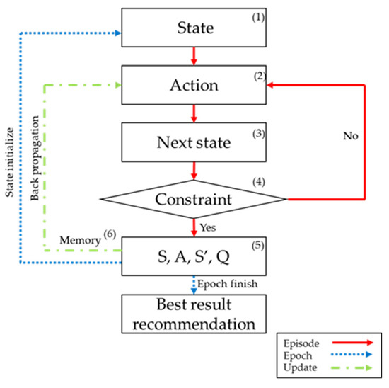
Figure 11. Deep RL algorithm procedure.

Episode (red solid line) selects “Action (2)” from “State (1)” and calculates “Next state (3).” If the calculated “Next state” meets “Constraint (4),” Episode ends and “State,” “Action,” “Next state,” and “Value (5)” are stored in “Memory (6).” If the constraint is not satisfied, “Action (2)” is executed again. Epoch (blue dotted line) saves the result from the completed Episode, initializes “State (1),” and suggests the optimal result when all epochs are completed. Update (green dotted line) updates “Action (2)” by sampling the batch from the memory after the episode ends and performing back propagation to reduce the loss function.

2.4. Applied Method

2.4.1. Shaft FE Modeling

To calculate the shaft reaction force and bending moment according to the offset, using the displacement of the aft stern tube bearing as a reference point, the shaft diameter change point, load action location, strain gauge attachment location, and node according to the bearing location were divided into nodes. The element details displayed in Table 8 were applied and modeled with the MSC software PATRAN, as illustrated in Figure 12.

Table 8. Shaft FE model details.

Description	Value
No. of nodes	54
No. of elements	53
Type of element	1D beam element
Young’s modulus [N/mm2]	$2.06\times {10}^5$
Poisson’s ratio	0.3

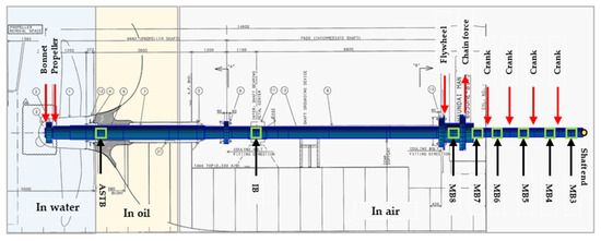
Figure 12. Shaft FE model.

Table 9 presents the applied loads in the drawing (bonnet and propeller) and recommended loads of the manufacturer (flywheel, chain force, and crank) acting on the shaft. Table 10 displays the boundary conditions of the nodes applied to the shaft model, and Table 11 presents the density information for calculating the density of the shaft in contact with seawater, lubricant, and air.

Table 9. Shaft FE model applied loads.

	Position [mm]	Load [kN]
Bonnet	290	8.813
Propeller	921	150.122
Flywheel	14,667	109.940
Chain force	15,375	−99.900
Crank	16,242	125.000
Crank	17,136	125.000
Crank	18,030	125.000
Crank	18,924	125.000

Table 10. Shaft FE model boundary conditions.

	Translations	Rotations
ASTB	Y, Z	-
IB	Y, Z	-
MB8	Y, Z	-
MB7	Y, Z	-
MB6	Y, Z	-
MB5	Y, Z	-
MB4	Y, Z	-
MB3	Y, Z	-
Shaft end	X, Y	X, Z

Table 11. Fluid density in contact with shaft FE model.

	Density [kg/mm3]	Start [mm]	End [mm]	Comments
Water density	$1.03\times {10}^{-9}$	0	1782	Bonnet, propeller
Oil density	$9.70\times {10}^{-10}$	1782	4902	ASTB
Shaft (in air)	$7.85\times {10}^{-9}$	4902	19,818	IB, MB, flywheel, crank

2.4.2. Deep RL Procedure

In this study, a deep RL algorithm was modeled in which a deep neural network was applied to a Q-learning algorithm for inverse analysis of the shaft deformation. Table 12 presents the hyperparameter values applied in this algorithm.

Table 12. Deep RL applied hyperparameters.

Category	Description	Value
Q-value	Learning rate ($\mathsf{\alpha }$)	0.001
	Discount factor ($\mathsf{\gamma }$)	0.95
$ϵ$-greedy policy	$ϵ$	0.05~0.01
Experience replay memory	Memory size	200
	Batch size	10
Deep neural network	Hidden layer	3
	Hidden layer node	128
	Activation function	ReLU
	Epoch	1000
	Loss	Mean squared error (MSE)
	Optimizer	Adam

The detailed procedure of the deep RL algorithm for applying the shaft deformation, as illustrated in Figure 8, is outlined as follows:

• State:

The state is a total of 12 variables, which are the reaction force of each bearing (ASTB, IB, MB8, MB7, and MB6) and the bending moment of the strain gauge attachment point (SG1–7). According to the measurement method, the variables constituting the state can be divided into three types: the directly measured reaction force (IB, MB8, MB7, and MB6), directly measured bending moment (SG1–7), and indirectly calculated reaction force from the bending moment using the moment equilibrium equation (ASTB).

2.

Action:

Based on the previous state, three vertical displacement variables of IB, MB8, and MB3 are output through the deep neural network, as illustrated in Figure 13. The displacement ASTB, which is not computed through the deep neural network, is 0 as the reference point of the shaft, and the main bearings MB7 to MB4 are linearly aligned. Thus, a total of eight vertical displacements (ASTB, IB, MB8, MB7, MB6, MB5, MB4, and MB3) are applied as inputs of the next state by linear interpolation between MB8 and MB3.

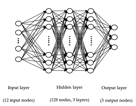
Figure 13. Action decision deep neural network.

3.

Next state:

The next state is the bearing reaction force and bending moment at the strain gauge point that is obtained by applying the vertical displacement of each bearing (action) to the shaft model and implementing the FE method.

4.

Constraint:

The constraint is the allowable condition of each bearing according to the classification regulations and manufacturer standard [29,30,31], the expression of which is equivalent to Equation (9):

$$constraint=\{\begin{array}{c}{\theta }_{ASTB}\le 0.3mrad\\ P_{min}\le P_b<P_{max}\\ \frac{{\delta }_{MB}{}_i-{\delta }_{MB}{}_j}{l_i-l_j}=constant \left(i,j in MB number, i\ne j\right)\\ {\delta }_{IB}>{\delta }_{MBaft}\end{array},$$

(9)

where ${\theta }_{ASTB}$ is the relative slope angle of the ASTB, $P_{min}$ is the minimum allowable bearing reaction force, $P_{max}$ is the maximum allowable bearing reaction force, $P_b$ is the bearing reaction force, $l$ is the bearing position, ${\delta }_{MB}$ is the MB displacement, ${\delta }_{IB}$ is the IB displacement, and ${\delta }_{MBaft}$ is the aftmost MB displacement.

According to the classification rules, as illustrated in Figure 14, the relative slope angle of the support point of the ASTB should be less than 0.3 mrad, and it is recommended that the surface pressure of the ASTB and IB does not exceed the allowable value [29,30,31].

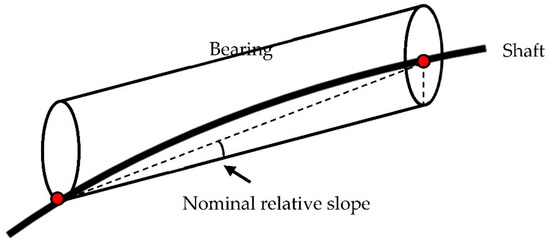
Figure 14. Stern tube bearing relative slope angle.

Table 13 presents the allowable reaction force of the ASTB and the IB of the target vessel, reflecting the classification rules.

Table 13. Allowable reaction force for bearings according to classification rules (ASTB, IB).

	Max. Permissible Pressure [MPa]	Bearing Area (Diameter $\times$[${\mathit{m}}^2]$ ([$\mathit{m}\times \mathit{m}\left]\right)$	Max. Ppermissible Load [kN]	Min. Permissible Load [kN]
ASTB	0.8	0.46 ($0.50\times 0.92$)	368.0	-
IB	1.2	0.1335 ($0.445\times 0.$30)	160.2	-

Furthermore, it is recommended by the manufacturer of the main engine of the target ship that the surface pressure of the MBs does not exceed the allowable value. Table 14 presents the allowable reaction force of the MBs, reflecting the recommendations of the main engine manufacturer.

Table 14. Allowable bearing reaction force according to recommendations of main engine manufacturer (MBs).

	Max. Permissible Load [kN]	Min. Permissible Load [kN]
MB8	336.0	0.0
MB7	336.0	17.0
MB6	336.0	17.0
MB5	336.0	17.0
MB4	336.0	17.0
MB3	336.0	17.0

According to the main engine manufacturer standard, the displacements of the MBs should be arranged linearly. Moreover, the displacement of the MB at the end of the stern should be located lower than the displacement of the IB [32].

5.

Value

The value refers to learning while repeating epochs and acting in the direction with the smallest difference from the actual measured value within minimum episodes. If deep RL is performed using the measured value as it is, the bending moment with a relatively large number of variables will have the greatest effect. However, as the criterion in the classification rules is the allowable reaction force of each bearing, deep RL was performed by applying a weight to the bearing reaction force [29,30,31]. In this study, the state variables were divided into three types: the direct measurement reaction force, direct measurement bending moment, and indirect calculation reaction force. As per Equation (10), weights of 0.55 for the directly measured bearing reaction force, 0.40 for the directly measured strain gauge bending moment, and 0.05 for the indirectly calculated bearing reaction force were applied to increase the priority of the jack-up reaction force during the deep RL.

$$\begin{gathered} Value=-1\cdot [0.55\cdot {{\displaystyle \sum }}^{ }\left(\left|R_{JU}-R_{JUmeasured}\right|\right)+0.40\cdot {{\displaystyle \sum }}^{ }\left(\left|M_{SG}-M_{measured}\right|\right) \\ +0.05\cdot {{\displaystyle \sum }}^{ }\left(\left|R_{ATSB}-R_{ASTBcalculated}\right|\right)] \end{gathered}$$

(10)

where $R_{JU}$ and $R_{JUmeasured}$ are the predicted and measured reaction force of IB, MB8, MB7, and MB6, $M_{SG}$ and $M_{measurement}$ are the predicted and measured bending moments of strain gages 1–7, and $R_{ASTB}$ and $R_{ASTBmeasured}$ are the predicted and calculated reaction forces of the aft stern tube bearing.

The goal of deep RL is to maximize the value, but the smaller the value calculated in Equation (10), the closer to the actual value, the closer the shaft deformation including the reaction force and bending moment is predicted. Therefore, the weighted sum is multiplied by –1 to predict the shaft deformation including the reaction force and bending moment close to the actual value.

6.

Memory

The memory stores the state, action, next state, and value at the end of an episode up to the maximum memory size and performs back propagation to obtain the action that maximizes the value using the batch that is extracted by sampling from memory, so that the update is focused on the most recent value.

3. Results

3.1. Deep RL Results

3.1.1. Light Draft Condition (D1)

To understand the trends of the shaft deformation prediction results after performing the deep RL inverse analysis under each draft condition, “offset” (a) (shaft deformation predicted by deep RL execution as the basis of the measured value), “load” (b) and “bending moment” (c) (reaction force and bending moment calculated by applying the shaft deformation to the finite element model), and “value” (d) (the difference between the predicted and measured values, where a smaller value is closer to the measured value) for all cases (Figure 15), the top 100 cases (Figure 16), and top 10 cases (Figure 17) are presented according to the “value” in the light draft condition (D1).

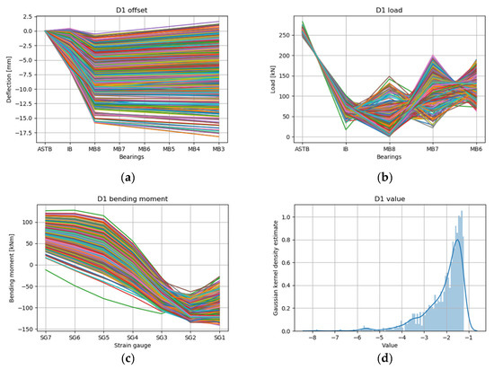
Figure 15. RL results for draft condition D1 all cases: (a) offset, (b) load, (c) bending moment, and (d) value.

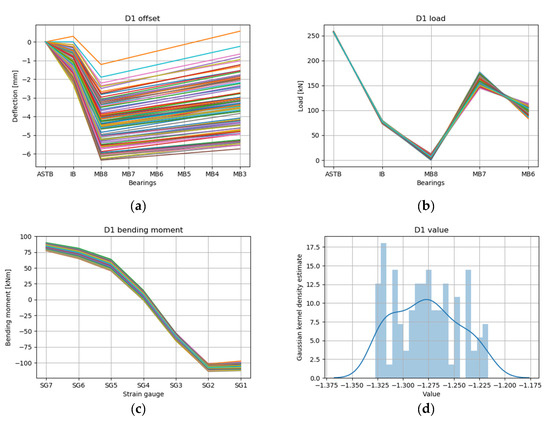
Figure 16. RL results for draft condition D1 top 100 cases: (a) offset, (b) load, (c) bending moment, and (d) value.

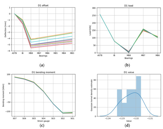
Figure 17. RL results for draft condition D1 top 10 cases: (a) offset, (b) load, (c) bending moment, and (d) value.

According to Figure 15, Figure 16 and Figure 17, which present the RL results of the light draft condition D1, the reaction force converged to a certain range with the filtering from all cases to the top 10 cases. The values in the top 10 cases (Figure 17d) were −1.23 to −1.22 and there was no significant difference in the values of the 10 cases, but the shaft deformation prediction (Figure 17a) did not converge beyond a certain level. Based on these results, various margins of error may occur in the shaft assembly stage depending on the sag tolerance of the engine bed plate, the deviation of the center of the MBs, and the tendency of the operator when the shaft installation is inclined compared to the design [12]. Owing to the above characteristics of the shaft, the fact that the reaction force and bending moment values in the shaft deformation prediction converged to similar values while filtering from all cases to the top 10 cases means that all shaft deformation predictions of the top 10 cases were valid. It is believed that the suggestion of the corresponding shaft deformation prediction range can aid the operator in decision-making during the process.

The shaft deformation, reaction force, bending moment predictions, and values of the top 10 cases according to the values in draft conditions D2–D5 are presented in the following.

3.1.2. Ballast Draft Conditions (D2 and D3)

The RL results of the ballast conditions D2 and D3 are depicted in Figure 18 and Figure 19, respectively. As in D1, the predicted values of the reaction force (Figure 18b and Figure 19b) and bending moment (Figure 18c and Figure 19c) in the top 10 cases converged to a certain range. The values of the 10 cases (Figure 18d and Figure 19d) were −2.45 to −2.35 in D2 and −2.50 to −2.30 in D3, and there was no significant difference among the values. It can be observed that the shaft deformation of D3 with the APT full (Figure 19a; IB: −0.2 to −0.8 mm; MB8: −1.6 to −3.2 mm; MB3: 0.2 to −1.9mm) was increased compared to the shaft deformation of D2 with the APT empty (Figure 18a; IB: −0.6 to −1.7 mm; MB8: −3.0 to −5.3 mm; MB3: −1.8 to −4.5 mm). As illustrated in Figure 5, it was estimated that the APT located at the stern of the target ship was full and the load on the rear part of the shaft increased, so that the shaft tended to increase relative to the ASTB.

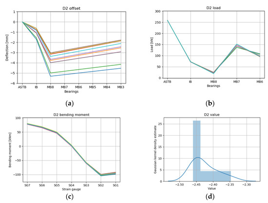
Figure 18. RL results for draft condition D2 top 10 cases: (a) offset, (b) load, (c) bending moment, and (d) value.

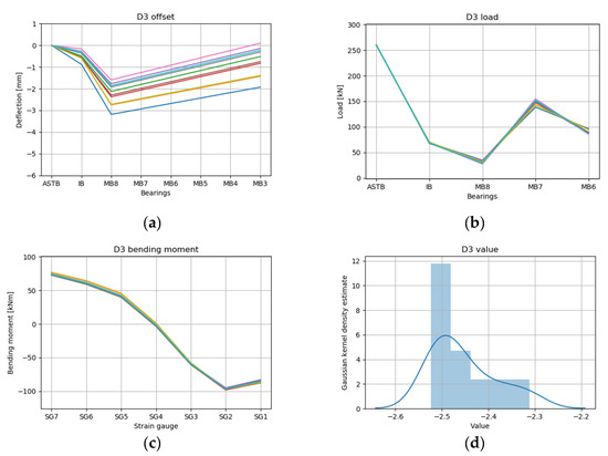
Figure 19. RL results for draft condition D3 top 10 cases: (a) offset, (b) load, (c) bending moment, and (d) value.

3.1.3. Scantling Draft Conditions (D4 and D5)

The RL results of the scantling conditions D4 and D5 are depicted in Figure 20 and Figure 21, respectively. As with the other results, the predicted values of the bending moment (Figure 20c and Figure 21c) in the top 10 cases converged to a certain range. The values of the 10 cases (Figure 20d and Figure 21d) were from −8.75 to −8.60 in D4 and from −5.95 to −5.65 in D5, and there was no significant difference among the values of the 10 cases. However, it can be observed that the predicted value of the reaction force according to the shaft deformation did not converge compared to the predicted reaction force values at other drafts in the MB, and the value was estimated to be larger than the values at other drafts.

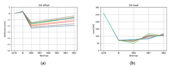
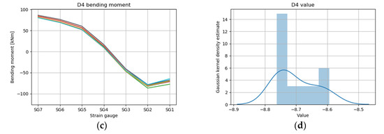
Figure 20. RL results for draft condition D4 top 10 cases: (a) offset, (b) load, (c) bending moment, and (d) value.

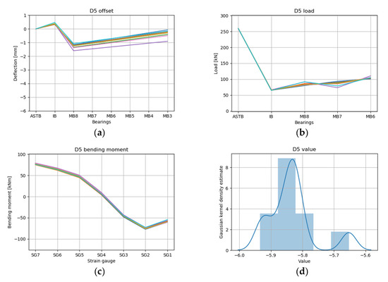
Figure 21. RL results for draft condition D5 top 10 cases: (a) offset, (b) load, (c) bending moment, and (d) value.

A small difference was observed compared to the difference in the shaft deformation depending on whether or not the APT was loaded in the ballast condition. However, the shaft deformation of D5 with the APT full (Figure 21a; IB: 0.5 to 0.4 mm; MB8: −1.1 to −1.6 mm; MB3: −0.1 to −0.9 mm) was increased compared to the shaft deformation of D4 with the APT empty (Figure 20a; IB: 0.4 to 0.3 mm; MB8: −1.4 to −2.3 mm; MB3: −0.4 to −1.9 mm). As in the ballast condition illustrated in Figure 5, it was estimated that the APT located at the stern of the target ship was full and the load on the rear part of the shaft increased, so that the shaft tended to rise relative to the ASTB.

However, as indicated in Figure 5c, compared to the ballast condition in which the APT was located above the water surface and the load was applied to the rear of the shaft, the scantling condition was as illustrated in Figure 5e, where the APT was mostly immersed in the lower portion of the water surface, and the load acting on the back of the shaft was estimated to have a small effect on the shaft deformation.

As a result of deep RL, the predicted reaction force, bending moment, and value converged to an almost certain range in the top 10 cases. As indicated in Table 15, the predicted shaft deformation occurred in the top 10 cases, but overall, as the load progressed from a light load to a full load draft, and when the aft peak tank changed from empty to full, the predicted shaft deformation tended to increase. Furthermore, the change in the shaft deformation owing to the loading of the APT was larger in the ballast condition than in the scantling condition.

Table 15. Shaft deformation prediction range.

	IB		MB8		MB3
	Min. [mm]	Max. [mm]	Min. [mm]	Max. [mm]	Min. [mm]	Max. [mm]
D1	−1.7	−1.0	−5.5	−4.0	−4.8	−3.0
D2	−1.7	−0.6	−5.3	−2.9	−4.5	−1.8
D3	−0.8	−0.2	−3.2	−1.5	−2.9	0.2
D4	0.3	0.5	−2.3	−1.4	−1.9	−0.5
D5	0.4	0.5	−1.6	−1.1	−0.9	0.0

3.2. Comparison of Predicted Results and Measurements

As a result of the shaft deformation prediction using the deep RL described in Section 3.1, the reaction force and bending moment within a certain range were converged in the top 10 cases. To compare these results with the actual measured values, the predicted value at the time of the best value was extracted and analyzed, as illustrated in Figure 22 and Figure 23.

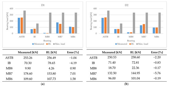
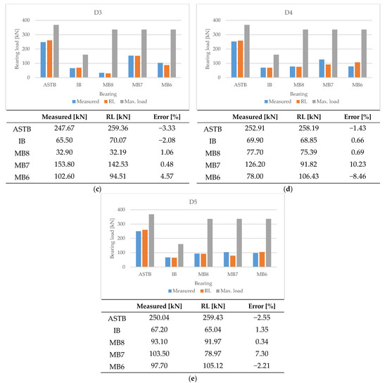
Figure 22. Comparison of predicted bearing reaction force with measurements of (a) D1, (b) D2, (c) D3, (d) D4, and (e) D5.

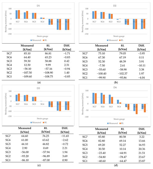
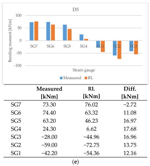
Figure 23. Comparison of predicted strain gauge bending moment with measurements of (a) D1, (b) D2, (c) D3, (d) D4, and (e) D5.

3.2.1. Comparison of Predicted Bearing Reaction Force with Measurements

The measured bearing reaction force, the reaction force in the shaft deformation predicted by deep RL, and the maximum allowable load on the bearings are depicted in Figure 22. As in Equation (11), where Error is the ratio of the difference between the measured and the predicted reaction force to the allowable bearing load.

$$Error=\left(Measured-RL\right)/\left(Max. load\right)$$

(11)

The calculated bearing reaction force in the predicted shaft deformation is similar to the measured value. Therefore, the inverse analysis technique applying deep RL predicted the shaft deformation in which the bearing reaction force was sufficiently reflected.

3.2.2. Comparison of Predicted Strain Gauge Bending Moment with Measurements

As illustrated in Figure 23, the calculated value of the strain gauge bending moment at the predicted shaft deformation was predicted similarly to the measured strain gauge bending moment.

In the scantling draft conditions D4 and D5, the predicted bending moment was overall lower than the measured value from the strain gauge by more than 10 kNm overall. However, the changes in the bending moment between strain gage positions predicted by deep RL under the draft conditions are similar to the changes in the measured values. Thus, the inverse analysis technique applied with deep RL predicted shaft deformation that sufficiently reflects the bending moment of the strain gage position, but predicted an overall low bending moment under some draft conditions.

3.3. Comparison with Previous Research Methods

The measured values and ship information used for the deep RL in this study were the same data as those in Lee [11]. The prediction results of the inverse analysis technique using the experimental method of Lee [11] and the inverse analysis technique using deep RL in this study were compared for each draft condition (D1 to D5). Figure 24 and Figure 25 present the comparison results of the measured values under each draft condition, the predicted values of the inverse analysis technique using deep RL, and the predicted values of the inverse analysis technique using the experimental method (EM).

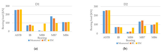
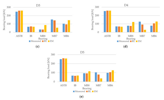
Figure 24. Comparison of reaction force prediction of (a) D1, (b) D2, (c) D3, (d) D4, and (e) D5.

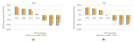
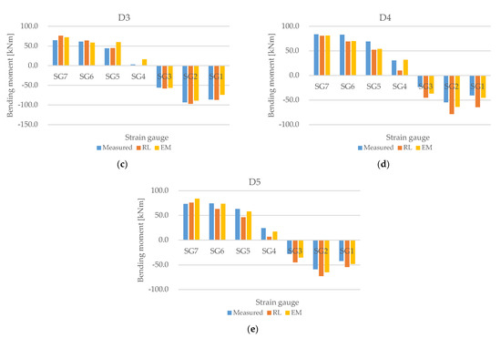
Figure 25. Comparison of bending moment prediction of (a) D1, (b) D2, (c) D3, (d) D4, and (e) D5.

The comparison results of the reaction force prediction in Figure 24 demonstrate that the reaction force predicted by the inverse analysis method using deep RL under all draft conditions was close to the measured MB reaction force value. The MB reaction force predicted by the inverse analysis method using the experimental method was significantly different from the measured MB reaction force value.

Previous inverse analysis studies by Rao et al. [10] and Šverko [3] also exhibited difficulties in predicting the MB reaction force. In particular, in the work of Šverko [3], inverse analysis was conducted with a genetic algorithm using the MB reaction force and strain gauge bending moment, as in this study, but it was difficult to predict the MB reaction force. Lee [11] discussed the difficulty of predicting the reaction force of the MB when predicting the shaft deformation because a difference in the reaction force occurs even with a small offset difference owing to the characteristics of the MB with a large reaction force influence coefficient. Nevertheless, the MB reaction force in the shaft deformation predicted by the inverse analysis technique using deep RL was closer to the actual measured value compared to the techniques used in the previous studies.

The comparison results of the bending moment prediction in Figure 25 demonstrate that in the light and ballast conditions (D1–D3), the inverse analysis technique using deep RL predicted values that were closer to the measured strain gauge bending moment value than the values of the inverse analysis technique using the experimental method. In the scantling conditions D4 and D5, the inverse analysis method using the experimental method predicted the bending moment closer to the measured strain gauge bending moment value than the inverse analysis method using deep RL.

The changes in the bending moment between strain gage positions predicted by deep RL under the draft conditions are similar to the changes in the measured values. The inverse analysis technique applied with deep RL predicted shaft deformation that sufficiently reflects the bending moment of the strain gage position but predicted an overall low bending moment under some draft conditions. Future research intends to advance the inverse analysis algorithm by applying deep RL as a supplement.

4. Discussion

In this study, deep RL, which has been used in various fields in recent years, was applied to the shaft inverse analysis technique to predict the shaft deformation according to the hull deformation. Moreover, the prediction results and those of previously conducted inverse analysis were compared and analyzed. The novelty of this study is the reasonable prediction of the shaft deformation of the MB, which was difficult in previous studies owing to the large reaction force influence coefficient and the resulting change in the reaction force compared to other bearings. As a result, it is expected that accurate shaft deformation prediction will be possible, while saving time and costs compared to existing methods.

In this study, the shaft deformation according to the draft was predicted by applying the reaction force measured by the jack-up method, which is the simplest and most accurate direct measurement method that can be used only when the shaft is stopped, and the bending moment measured by the strain gauge method, which is time consuming, and can be used even when rotating the shaft, to the inverse analysis technique using deep RL. Moreover, the effect of the hull deformation according to the draft change on the shaft deformation was examined without shaft rotation; that is, in the static state. However, unlike in the static shaft state, in the dynamic shaft state, it is difficult to measure the bearing reaction force using a hydraulic jack, and the effects of the thrust that is generated from the propeller during ship operation on the propulsion shaft system should be investigated.

Therefore, future research will include the performance of cross-validation of the strain gauge method and the jack-up method to guarantee the accuracy of the strain gauge method. Subsequently, the strain gauge method will be applied to the inverse analysis technique using deep RL to predict the shaft deformation in the dynamic state of a vessel in operation.

5. Conclusions

In this study, the bearing reaction force and bending moment were measured according to the draft conditions in the static shaft of a 50,000 DWT medium-sized oil/chemical tanker equipped with a high-efficiency engine. The inverse analysis technique was modeled using deep RL, and the following results were obtained by predicting the shaft deformation from the measured values under five draft conditions:

• Although the predictions of the shaft deformation of the top 10 cases were not exactly the same, the predicted values of the reaction force and bending moment converged within a certain range.
• For each draft condition, the predicted shaft deformation tended to increase as the target ship progressed from a light load to a full load.
• Under the same draft condition, the shaft deformation tended to increase in the state where the APT was full compared to the state in which the APT was empty. It was estimated that the load of the APT located at the stern was applied on the rear part of the shaft.
• A rise of the shaft owing to the loading of the APT occurred significantly in the ballast condition compared to the scantling condition. It was estimated that this was because the APT was located above the water surface and the load that was applied on the rear part of the shaft was larger than that in the scantling condition.
• In this study, the shaft deformation that sufficiently reflects the measured MB reaction force was predicted, which was difficult in previous inverse analysis studies owing to the large reaction force influence coefficient.
• The aim of future research will be to confirm the validity of the strain gauge method based on the static shaft deformation prediction applied in this study, so as to use the method for dynamic shaft deformation prediction through the advancement of the inverse analysis technique with deep RL.

References

- Mangesh, V.L.; Mohan, A. effective EEDI performance achievement by MAN B&W G-type ultra long stroke marine diesel engine: A review. Int. J. Veh. Struct. Syst. 2017, 9, 269–272. [Google Scholar] [CrossRef]
- Vartdal, B.J.; Gjestland, T.; Arvidsen, T.I. Lateral propeller forces and their effects on shaft bearings. In Proceedings of the First International Symposium on Marine Propulsors, Trondheim, Norway, 22–24 June 2009; pp. 475–481. [Google Scholar]
- Šverko, D. Design concerns in propulsion shafting alignment. In Proceedings of the ICMES Conference 2003, Helsinki, Finland, 19–21 May 2003. [Google Scholar]
- Šverko, D. Hull deflections shaft alignment interaction, a case study. In Proceedings of the 7th International Symposium on Marine Engineering, Tokyo, Japan, 24–28 October 2005; pp. 245–251. [Google Scholar]
- Murawski, L. Shaft line alignment analysis taking ship construction flexibility and deformations into consideration. Mar. Struct. 2005, 18, 62–84. [Google Scholar] [CrossRef]
- Shi, L.; Xue, D.; Song, X. Research on shafting alignment considering ship hull deformations. Mar. Struct. 2010, 23, 103–114. [Google Scholar] [CrossRef]
- Choung, J.-M.; Choe, I.-H. Development of elastic shaft alignment design program. J. Soc. Nav. Archit. Korea 2006, 43, 512–520. [Google Scholar] [CrossRef]
- Korbetis, G.; Vlachos, O.; Charitopoulos, A.G.; Papadopoulos, C.I. Effects of hull deformation on the static shaft alignment characteristics of VLCCs: A case study. In Proceedings of the 13th International Conference on Computer Applications and Information Technology in the Maritime Industries, Redworth, UK, 12–14 May 2014; pp. 546–557. [Google Scholar]
- Seo, C.-O.; Jeong, B.; Kim, J.-R.; Song, M.; Noh, J.-H.; Lee, J. Determining the influence of ship hull deformations caused by draught change on shaft alignment application using FE analysis. Ocean. Eng. 2020, 210, 107488. [Google Scholar] [CrossRef]
- Rao, M.N.K.; Dharaneepathy, M.V.; Gomathinayagam, S.; Ramaraju, K.; Chakravorty, P.K.; Mishra, P.K. Computer-Aided Alignment of Ship Propulsion Shafts by Strain-Gage Methods. Mar. Technol. SNAME News 1991, 28, 84–90. [Google Scholar] [CrossRef]
- Lee, J.-U. A study on the analysis of bearing reaction forces and hull deflections affecting shaft alignment using strain gauges for a 50,000 DWT oil/chemical tanker. J. Korean Soc. Mar. Eng. 2016, 40, 288–294. [Google Scholar] [CrossRef]
- Sharifi, A.; Mohebbi, A. introducing a new formula based on an artificial neural network for prediction of droplet size in venturi scrubbers. Braz. J. Chem. Eng. 2012, 29, 549–558. [Google Scholar] [CrossRef]
- Sutton, R.S.; Barto, A.G. Reinforcement Learning: An Introduction; MIT Press: Cambridge, MA, USA, 2018. [Google Scholar]
- Uyanik, T.; Karatuğ, Ç.; Arslanoğlu, Y. Machine learning approach to ship fuel consumption: A case of container vessel. Transp. Res. D Transp. Environ. 2020, 84, 102389. [Google Scholar] [CrossRef]
- Cheliotis, M.; Lazakis, I.; Theotokatos, G. Machine Learning and data-driven fault detection for ship systems operations. Ocean. Eng. 2020, 216, 107968. [Google Scholar] [CrossRef]
- Kim, Y.-R.; Jung, M.; Park, J.-B. Development of a fuel consumption prediction model based on machine learning using ship in-service data. J. Mar. Sci. Eng. 2021, 9, 137. [Google Scholar] [CrossRef]
- Song, J.; Kim, D.-J.; Kang, K.-M. Automated procurement of training data for machine learning algorithm on ship detection using AIS information. Remote Sens. 2020, 12, 1443. [Google Scholar] [CrossRef]
- Karvelis, P.; Georgoulas, G.; Kappatos, V.; Stylios, C. Deep machine learning for structural health monitoring on ship hulls using acoustic emission method. Ships Offshore Struct. 2021, 16, 440–448. [Google Scholar] [CrossRef]
- Scardua, L.A.; Da Cruz, J.J.; Costa, A.H.R. Optimal control of ship unloaders using reinforcement learning. Adv. Eng. Inform. 2002, 16, 217–227. [Google Scholar] [CrossRef]
- Fu, K.; Li, Y.; Sun, H.; Yang, X.; Xu, G.; Li, Y.; Sun, X. A ship rotation detection model in remote sensing images based on feature Fusion pyramid network and deep reinforcement learning. Remote Sens. 2018, 10, 1922. [Google Scholar] [CrossRef] [Green Version]
- Zhao, L.; Roh, M. COLREGs-compliant multiship collision avoidance based on deep reinforcement learning. Ocean. Eng. 2019, 191, 106436. [Google Scholar] [CrossRef]
- Lee, Y.-J.; Kim, U.-K. A Study on hull deflection and shaft alignment interaction in VLCC. J. Korean Soc. Mar. Eng. 2005, 29, 73–82. [Google Scholar]
- Wang, S.-C. Artificial neural network. In Interdisciplinary Computing in Java Programming; The Springer International Series in Engineering and Computer Science; Springer: Boston, MA, USA, 2003; Volume 743, pp. 81–100. [Google Scholar]
- Bellman, R. Dynamic Programming. Science 1966, 153, 34–37. [Google Scholar] [CrossRef] [PubMed]
- Watkins, C.J.C.H.; Dayan, P. Q-Learning. Mach. Learn. 1992, 8, 279–292. [Google Scholar] [CrossRef]
- Cheng, Z.; Zhao, Q.; Wang, F.; Jiang, Y.; Xia, L.; Ding, J. Satisfaction based Q-learning for integrated lighting and blind control. Energy Build. 2016, 127, 43–55. [Google Scholar] [CrossRef]
- Mnih, V.; Kavukcuoglu, K.; Silver, D.; Graves, A.; Antonoglou, I.; Wierstra, D.; Riedmiller, M. Playing Atari with Deep Reinforcement Learning. arXiv 2013, arXiv:1312.5602. [Google Scholar]
- Lin, L.-J. Self-improving reactive agents based on reinforcement learning, planning and teaching. Mach. Learn. 1992, 8, 293–321. [Google Scholar] [CrossRef]
- DNV, G.L. Rules for Classification: Ships Part 4 Chapter 2. Available online: https://rules.dnv.com/docs/pdf/DNV/RU-SHIP/2020-10/DNVGL-RU-SHIP-Pt1Ch2.pdf (accessed on 1 June 2021).
- Lloyd’s Register. Rules and Regulations for the Classification of Ships. Available online: https://www.lr.org/en/rules-and-regulations-for-the-classification-of-ships/ (accessed on 1 June 2021).
- ABS. Guidance Notes on ’Propulsion Shafting Alignment’. Available online: https://ww2.eagle.org/content/dam/eagle/rules-and-guides/current/design_and_analysis/128_propulsionshaftalignment/shaft-alignment-gn-sept-19.pdf (accessed on 1 June 2021).
- MAN Diesel & Turbo. Bearing Load Measurement by Jacking Up; MDT: Copenhagen, Denmark, 2012. [Google Scholar]
Publisher’s Note: MDPI stays neutral with regard to jurisdictional claims in published maps and institutional affiliations. |
© 2021 by the authors. Licensee MDPI, Basel, Switzerland. This article is an open access article distributed under the terms and conditions of the Creative Commons Attribution (CC BY) license (https://creativecommons.org/licenses/by/4.0/).