Particle-Swarm-Optimization-Enhanced Radial-Basis-Function-Kernel-Based Adaptive Filtering Applied to Maritime Data

Abstract

The real-life signals captured by different measurement systems (such as modern maritime transport characterized by challenging and varying operating conditions) are often subject to various types of noise and other external factors in the data collection and transmission processes. Therefore, the filtering algorithms are required to reduce the noise level in measured signals, thus enabling more efficient extraction of useful information. This paper proposes a locally-adaptive filtering algorithm based on the radial basis function (RBF) kernel smoother with variable width. The kernel width is calculated using the asymmetrical combined-window relative intersection of confidence intervals (RICI) algorithm, whose parameters are adjusted by applying the particle swarm optimization (PSO) based procedure. The proposed RBF-RICI algorithm’s filtering performances are analyzed on several simulated, synthetic noisy signals, showing its efficiency in noise suppression and filtering error reduction. Moreover, compared to the competing filtering algorithms, the proposed algorithm provides better or competitive filtering performance in most considered test cases. Finally, the proposed algorithm is applied to the noisy measured maritime data, proving to be a possible solution for a successful practical application in data filtering in maritime transport and other sectors.

1. Introduction

In today’s world, due to the advances in digital technologies, vast amounts of data are continuously acquired by different measurement systems, covering all fields of human activities. These data are then used as input to various algorithms and analysis procedures. However, the obtained real-life signals are often corrupted by various types of noise, which occur due to numerous environmental factors and to the data acquisition and transmission processes themselves. Therefore, prior to the further exploitation and analysis of such data, it needs to be processed by filtering algorithms to reduce the noise, thus enabling more efficient reconstruction of the original information content [1,2,3,4,5,6,7].

The modern maritime transport sector is an example of a complex system consisting of different measurement subsystems and communication systems used to transmit collected information. Moreover, the future development of autonomous shipping increases the amount of data acquired during the ship operation, thus placing additional demand on data quality. Maritime applications imply operation under difficult and rapidly changing environmental conditions, which, accompanied by the reduced availability of reliable communication channels, leads to high noise levels in the acquired data. Therefore, the implementation of the existing and the development of the application-specific filtering algorithms for the reconstruction of useful information from the noise-corrupted signals is an important field of scientific research within maritime and transport engineering [8]. The research has been focused on different areas of application, including underwater signal processing [9,10,11,12], radar signal processing [13,14], underwater image processing [15,16,17], optical signal processing [18], and other applications [19,20,21].

The parametric filtering algorithms require knowledge of the underlying signal and noise characteristics. In many practical applications, such information is not available, and nonparametric filtering algorithms are used [22]. The main task in these algorithms includes applying a method for finding the optimal filter width that controls the level of signal smoothing. The nonparametric methods may be broadly classified into the plug-in methods and the quality-of-fit methods (such as, for example, cross-validation) [22]. The plug-in methods are computationally demanding due to complex formulae for calculating the optimal filter width based on the estimation bias and variance. On the other hand, the data-driven cross-validation method does not require bias estimation. The optimal filter width minimizes the estimation mean squared error (MSE) resulting in an optimal bias-variance trade-off [22].

An easy-to-implement and locally adaptive filtering algorithm is based on the intersection of confidence intervals (ICI) rule [23] combined with the local polynomial approximation (LPA) [24,25]. The LPA-ICI algorithm requires only the estimation of the signal and noise variance. The ICI rule for the optimal filter width selection was upgraded in [26] and named the relative intersection of confidence intervals (RICI) rule, keeping the good properties of the ICI rule, and at the same time improving the filtering performance in terms of MSE and reducing method’s sensitivity to suboptimal parameter selection.

As it may be expected, the filtering performances of the LPA-ICI and the LPA-RICI algorithms are affected by selected parameters’ values. Different data-driven techniques have been analyzed for the selection of the ICI rule’s parameter [24]. However, the RICI algorithm requires a simultaneous adjustment of two parameters, which has not been investigated in depth in the literature. Therefore, the approach based on the grid search in parameter space is generally used when applying the RICI algorithm. The time-consuming nature of this procedure places a demand for a faster solution. The study in [27] proposed a simulation-based method for the selection of the appropriate values of the RICI rule’s parameters with respect to the obtained MSE. However, the provided empirical formula defines regions of near-optimal parameter values and is obtained by analyzing a limited number of signal classes. Moreover, the formula for the calculation of one parameter’s value requires the other parameter’s value as an input, thus leaving a problem of its proper selection. Therefore, a more general approach, which will guarantee the optimal parameters’ values, is required.

In this paper, we propose an adaptive filtering algorithm based on the radial basis function (RBF) kernel smoother with variable width. The kernel width is calculated using the asymmetrical combined-window RICI algorithm. This data-driven, locally adaptive algorithm requires only the noise variance estimation (and does not require the bias estimation nor any information about the underlying signal and noise). In order to reduce the time required by the procedure based on a grid search in the parameter space, the RICI algorithm is upgraded by the particle swarm optimization (PSO) based procedure. We analyze the proposed RBF-RICI algorithm’s filtering performance by applying it to several synthetic, simulated noisy signals. The paper elaborates on the RBF-RICI’s efficiency in noise suppression and the filtering error reduction. Moreover, we compare the proposed algorithm to the competing filtering algorithms and show that it provides better or competitive filtering performance in most considered test cases. Additionally, we have performed a comparative analysis of several evolutionary metaheuristic optimization algorithms applied to selecting the RBF-RICI algorithm’s parameters, including the genetic algorithm (GA) and three algorithms based on the PSO. Finally, the proposed RBF-RICI algorithm is applied to the noisy, real-life measured maritime data, proving to be a potential solution for a successful practical application in data filtering in the maritime and other similar sectors.

The rest of this paper is structured as follows. The proposed filtering algorithm and optimization procedures are described in Section 2. The obtained results are thoroughly presented and discussed in Section 3. Finally, the conclusions are summarized in Section 4.

2. Materials and Methods

We consider the noisy observations of signal $y\left(k\right)$:

$$y\left(k\right)=x\left(k\right)+n\left(k\right),$$

(1)

where $x\left(k\right)$ is the original signal, and $n\left(k\right)$ is the additive white Gaussian noise.

The noisy signal $y\left(k\right)$ has to be filtered in order to obtain the estimate of the original signal $\widehat{x}\left(k\right)$ with the minimum estimation error. In this work, we propose an adaptive filtering algorithm combining the RBF kernel smoother with the asymmetrical combined-window RICI procedure whose parameters are adjusted utilizing the PSO algorithm.

2.1. The RBF-Kernel-Based Adaptive Filtering

The kernel smoother estimates the signal sample value as the weighted average of the neighboring observed sample values. The weights assigned to the specific samples are determined by the kernel type. Nonrectangular kernels assign higher weights to the samples closer and smaller weights to the samples farther away from the considered one [28].

The RBF or Gaussian kernel $K(k_0,k,h)$ is defined as:

$$K(k_0,k,h)=e^{-\frac{{\left(k_0-k\right)}^2}{2{\sigma }^2}},$$

(2)

where $k_0$ is the sample of interest, k is the neighboring signal sample, h is the kernel width, and $\sigma$ is the RBF kernel scale which is referred to as standard deviation when considering the Gaussian probability density function.

The Nadaraya–Watson kernel-weighted estimate [29] of the signal value at the considered sample is given by:

$$\widehat{x}(k_0,h)=\frac{{\sum }_{k}K(k_0,k,h)y\left(k\right)}{{\sum }_{k}K(k_0,k,h)}.$$

(3)

The kernel width h is a parameter that controls the estimation accuracy and the smoothness of the estimated signal. The kernels with larger widths include more samples in the estimation procedure, causing the decreased estimation variance and, at the same time, increased estimation bias. On the other hand, smaller kernel widths lead to the increase in the estimation variance and, simultaneously, the decrease in the estimation bias due to the reduced number of samples taken into the estimation procedure [24].

Therefore, the selection of the proper kernel width determines the efficiency of the applied filtering algorithm. As opposed to the constant kernel width used for the entire duration of the signal, the varying kernel width enables the adaptation to the local signal features. The kernel width providing the optimal trade-off between estimation bias and variance is here calculated using the adaptive RICI algorithm.

The absolute value of error ${\epsilon }_n(k,h)$ obtained by the kernel-smoother-based estimation procedure is defined as:

$$\left|{\epsilon }_n(k,h)\right|=\left|x\left(k\right)-{\widehat{x}}_n(k,h)\right|,$$

(4)

where ${\widehat{x}}_n(k,h)$ represents the signal sample value estimated using n samples in its vicinity by applying the kernel with varying width $h\left(k\right)$.

The mean squared estimation error, $MSE(k,h)$, may be defined, with respect to the estimation bias $b_n(k,h)$ and the estimation variance ${\sigma }_n^2(k,h)$, as [30,31]:

$$MSE(k,h)=E\left\{{\epsilon }_n^2(k,h)\right\}={\left|b_n(k,h)\right|}^2+{\sigma }_n^2(k,h).$$

(5)

The crucial task of the adaptive filtering procedure includes selecting the kernel width $h^o\left(k\right)$ that minimizes $MSE(k,h)$, thus providing the optimal bias-variance trade-off [30,31]:

$$h^o\left(k\right)=\underset{h\left(k\right)}{\mathrm{argmin}}MSE(k,h).$$

(6)

Note that the original signal values $x\left(k\right)$ are with the confidence p contained within confidence intervals ${\delta }_n(k,h)$ [24,31]:

$${\delta }_n(k,h)=\left[{\delta }_{l,n}(k,h),{\delta }_{u,n}(k,h)\right],n=1,\dots ,N,$$

(7)

where ${\delta }_{l,n}(k,h)$ and ${\delta }_{u,n}(k,h)$ are the lower and the upper confidence limits, respectively. The confidence limits are defined using the ICI threshold parameter $\Gamma$ representing the critical value of the confidence interval:

$${\delta }_{l,n}(k,h)={\widehat{x}}_n(k,h)-\Gamma ·{\sigma }_n(k,h),$$

(8)

$${\delta }_{u,n}(k,h)={\widehat{x}}_n(k,h)+\Gamma ·{\sigma }_n(k,h).$$

(9)

The initial stage of the RICI algorithm is identical to the ICI rule [23], which provides a set of N growing kernel widths $H=\left\{h_1,h_2,\dots ,h_N\right\}, h_1<h_2<\dots <h_N$, and the corresponding confidence intervals ${\delta }_n(k,h)$ for each signal sample k [24,25,31].

The ICI rule algorithm tracks the intersection of the confidence intervals and provides the largest kernel width $h^{ICI}\left(k\right)$ for which the intersection still exists [24,25,31]:

$$h^{ICI}\left(k\right)=\underset{h_n\left(k\right)}{\mathrm{argmax}}\left\{{\cap }_{n=1}^N{\delta }_n(k,h_n)\ne \varnothing \right\}.$$

(10)

This condition is met if the inequality ${\overline{\delta }}_{l,n}(k,h)\le {\underline{\delta }}_{u,n}(k,h)$ is satisfied, where ${\overline{\delta }}_{l,n}(k,h)$ is the largest lower and ${\underline{\delta }}_{u,n}(k,h)$ is the smallest upper confidence limit [24,31].

In this work, we applied the asymmetrical combined-window RICI approach, where the above-described procedure is implemented independently to the left and right side of the considered sample k, resulting in two sets of confidence intervals ${\delta }^l(k,h)$ and ${\delta }^r(k,h)$ for each signal sample k [27].

The algorithm tracks the intersection of the currently calculated nth confidence interval with the intersection of all previous $n-1$ confidence intervals on the each side of the considered kth sample independently. This results in $h^{l,ICI}\left(k\right)$ and $h^{r,ICI}\left(k\right)$ as the largest kernel widths satisfying (10) for the left and right side, respectively [27]. Finally, the candidate for the optimal width of the asymmetrical kernel is obtained by combining $h^{l,ICI}\left(k\right)$ and $h^{r,ICI}\left(k\right)$:

$$h^{ICI}\left(k\right)=h^{l,ICI}\left(k\right)+h^{r,ICI}\left(k\right)-1.$$

(11)

The ICI algorithm’s performance is highly sensitive to the selection of the optimal value of the threshold parameter $\Gamma$, as too small values result in signal undersmoothing, and too large values cause signal oversmoothing [24,30].

In order to make the ICI rule stage more robust to suboptimal $\Gamma$ values, the second stage of the algorithm includes the RICI rule upgrade, which applies the additional criterion for the adaptive kernel width selection to the kernel width candidates obtained by the ICI rule. The RICI rule improves the estimation accuracy of the ICI rule for the same values of the threshold parameter $\Gamma$ [26,27,32,33].

The RICI criterion ${\lambda }_n(k,h)$ tracks the relative amount of confidence intervals overlapping by calculating the ratio of the intersection of the confidence intervals’ width and the current confidence interval’s width [26,27]:

$${\lambda }_n(k,h)=\frac{{\underline{\delta }}_{u,n}(k,h)-{\overline{\delta }}_{l,n}(k,h)}{{\delta }_{u,n}(k,h)-{\delta }_{l,n}(k,h)}.$$

(12)

The calculated RICI ratio ${\lambda }_n(k,h)$ is compared to the preset RICI threshold value ($0\le R_c\le 1$) [27]:

$${\lambda }_n(k,h)\ge R_c.$$

(13)

Similar to the ICI rule stage, the RICI rule is also applied independently to the both sides of the considered samples, resulting in $h^{l,RICI}\left(k\right)$ and $h^{r,RICI}\left(k\right)$ which are the largest kernel widths satisfying (10) and (13) for the left and right side, respectively [27]. Finally, the width of the asymmetrical kernel $h^{RICI}\left(k\right)$ obtained by the RICI algorithm is calculated as:

$$h^{RICI}\left(k\right)=h^{l,RICI}\left(k\right)+h^{r,RICI}\left(k\right)-1.$$

(14)

2.2. The Evolutionary Metaheuristic Optimization Algorithms

In real-world engineering applications, optimization problems are often nonlinear, NP-hard (nondeterministic polynomial time-hard), and nondifferentiable. The traditional techniques require a mathematical formulation of the considered problem, which is often not possible. However, the evolutionary metaheuristic optimization algorithms have been proved to be powerful tools for nonlinear optimization problems. They overcome the limitations of the traditional techniques for nondifferentiable, noncontinuous, and nonconvex objective functions. In this paper, we use and compare several evolutionary metaheuristic optimization algorithms based on the PSO and GA. The generalized pseudocodes for Algorithms A1–A4 are provided in Appendix A.

2.2.1. Traditional PSO Algorithm

The PSO is a population based iterative algorithm, where all particles are gathered in one population, called the swarm [34,35,36]. Each particle represents the potential solution of the optimization problem in the solution space. In each iteration, particles adjust its flying trajectories according to personal and global experiences. Let us denote parameter s as the number of particles, or the population size, and d as the dimension of the solution space. d-dimensional solution space is defined with problem variables that need to be optimized [34,35]. Particles move in the solution space by updating their velocity vector, which is for the i-th particle ($i\in [1,s]$) defined as $v_i=(v_{i,1},v_{i,2},\dots ,v_{i,d})$, and position vector of the i-th particle, $x_i=(x_{i,1},x_{i,2},\dots ,x_{i,d})$, according to the following equations:

$$v_{i,d}=w·v_{i,d}+c_1·r_1·(p_{i,d}-x_{i,d})+c_2·r_2·(p_{g,d}-x_{i,d}),$$

(15)

$$x_{i,d}=x_{i,d}+v_{i,d},$$

(16)

where $r_1$ and $r_2$ are random numbers sampled from the range 0 to 1, w is the inertia weight, $c_1$ and $c_2$ denote the acceleration coefficients which control the particle movement toward the personal and the global best, $p_{i,d}$ and $p_{g,d}$, respectively [34,35]. Apart from limiting particle positions for the constrained problem, the value of each velocity $v_{i,d}$ can be limited also to range $[v_{min,d},v_{max,d}]$ in order to reduce the likelihood of particles moving too fast in smaller solution spaces.

A suitable selection of the inertia factor and the acceleration coefficients provides a balance between global and local exploration and exploitation. Further research has claimed that improved PSO performance could be gained if the inertia weight was chosen as a linearly decreasing number rather than a constant number over all iterations. The idea was that PSO search should start with high inertia weight for strong global exploration while, with linearly decreasing, in later iterations emphasize finer local explorations [34,35]. The w used in our simulations is given as:

$$\begin{array}{c}\hfill w=w_{max}-(w_{max}-w_{min})\ast (it/MaxIt),\end{array}$$

(17)

where parameters $it$ and $MaxIt$ stand for the current and maximum PSO iteration, respectively [34,35].

2.2.2. Enhanced Partial Search Particle Swarm Optimization (EPS-PSO) Algorithm

In some cases, the standard PSO might lead to a stagnant state, meaning that the global best position cannot be improved over iterations. To avoid PSO’s convergence to a local optimum, a supplementary search direction was obtained by implementing an additional population that takes up the global search assignment. The PSO variation is termed as the Enhanced Partial Search Particle Swarm Optimization (EPS-PSO) [35].

At the start of the EPS-PSO algorithm, the entire population is divided equally into two subswarms, namely the traditional subswarm and the cosearch swarm, respectively. The main difference between those two swarms is that the cosearch swarm is periodically reinitialized every $t_g$ iterations, where $t_g$ is called the reinitialization period [35]. The reinitialization of the particle positions is performed uniformly in the search space. However, there is an exception; if the current global best position of the cosearch, denoted as $p_{CO-g,d}$, outperforms the global best position of the traditional swarm, denoted as $p_{T-g,d}$, then the reinitialization of the cosearch swarm is called off. Basically, two subswarms work independently. The only cooperation between the subswarms is when the cosearch swarm exploits better outcomes than the traditional swarm. In that case, the velocity vector of the traditional swarm will update its value based on the $p_{CO-g,d}$, instead of the $p_{T-g,d}$ [35].

2.2.3. Multiswarm Particle Swarm Optimization (MSPSO)

The Multiswarm Particle Swarm Optimization (MSPSO) algorithm is another variant PSO algorithm that also introduces additional swarms [37]. Therefore, the total population depends not only on the number of particles but also on the number of swarms, denoted as $nSwarm$. The number of swarms determines the degree of communication between the swarms. The studies have shown that the algorithm performance can be improved by involving more swarms in the process [35,37]. However, introducing more swarms also increases the number of evaluations. For our optimizations, we have divided the same population size of the previous PSO variants into multiple swarms.

2.2.4. Genetic Algorithm (GA)

The GA is a stochastic algorithm invented to mimic some procedures in the natural evolution [36]. In GA, new particles, also called offsprings, are formed by combining two particles from current generations, called parents, using crossover and mutation operators. A new generation is formed by keeping the best performing particles from the parents and offsprings. The crossover and mutation operators are part of genetic operators based on the Darwinian principle of survival of the best performing particle in the population. In the GA used in this paper, the numbers of offspring and mutants, $n_c$ and $n_m$ respectively, are controlled with parameters $p_c$ and $p_m$ [36].

3. Results and Discussion

In order to investigate the efficiency of the proposed RBF-RICI adaptive filtering algorithm, we have applied it to the several synthetic signals, including Blocks, Bumps, Doppler, HeaviSine, Piece-Regular, and Sing signal. These signals are chosen as they represent good models of some typical real-world data found in various engineering and signal processing applications. For example, the piecewise constant Blocks signal is used as a model of the acoustic impedance of a layered medium in geophysics or of the one-dimensional profile along certain images in image processing applications [38]. Moreover, the Bumps signal represents spectra arising in nuclear magnetic resonance (NMR), absorption, and infrared spectroscopy [38], whereas the Piece-Regular signal is similar to wave arrivals in a seismogram. Each considered signal is corrupted by the white additive Gaussian noise and studied for three cases corresponding to signal-to-noise-ratio (SNR) values of 5, 7, and 10 dB.

The RBF-RICI algorithm is also compared to the zero-order LPA-RICI, the original LPA-ICI, and the Savitzky–Golay [39] filtering algorithms. To facilitate the quantitative analysis of the tested algorithms, the following filtering quality indicators were calculated for signals of the length $N_k$:

Mean squared error (MSE):

$$MSE=\frac{1}{N_k}\sum _{k=1}^{N_k}{\left(x\left(k\right)-{\widehat{x}}_n\left(k\right)\right)}^2,$$

(18)

Mean absolute error (MAE):

$$MAE=\frac{1}{N_k}\sum _{k=1}^{N_k}\left|x\left(k\right)-{\widehat{x}}_n\left(k\right)\right|,$$

(19)

Maximum absolute error (MAXE):

$$MAXE=\underset{k=1,\dots ,N_k}{max}\left|x\left(k\right)-{\widehat{x}}_n\left(k\right)\right|,$$

(20)

Peak signal-to-noise ratio (PSNR):

$$PSNR=20{log}_{10}\left(\frac{{max}_{k=1,\dots ,N_k}x\left(k\right)}{\sqrt{\frac{1}{N_k}{\sum }_{k=1}^{N_k}{\left(x\left(k\right)-{\widehat{x}}_n\left(k\right)\right)}^2}}\right),$$

(21)

Improvement in the signal-to-noise ratio (ISNR):

$$ISNR=10{log}_{10}\left(\frac{{\sum }_{k=1}^{N_k}{\left(x\left(k\right)-y\left(k\right)\right)}^2}{{\sum }_{k=1}^{N_k}{\left(x\left(k\right)-{\widehat{x}}_n\left(k\right)\right)}^2}\right).$$

(22)

The RBF-RICI algorithm, as well as the other tested algorithms, are applied with the optimal parameters for each considered signal, i.e., the parameters that minimize the estimation MSE. The optimal parameter values of the LPA-ICI algorithm are found in the range of $0\le \Gamma \le 5$. The Savitzky–Golay filtering algorithm is applied with the second order polynomial and the optimal window width h. The optimal parameters of the RBF-RICI and LPA-RICI algorithms are found by running the exhaustive grid search in the parameter space defined by parameters’ value ranges of $0\le \Gamma \le 5$ and $0\le R_c\le 1$. The search is conducted with the fine parameter value resolution of ${10}^{-2}$, resulting in the total number of 50,000 iterations and algorithm evaluations. To speed up this time-consuming and strenuous process, the PSO algorithm is proposed in the RBF-RICI parameters optimization. Different PSO algorithm realizations, as well as the genetic algorithm, are tested, and their performances are compared. The obtained results are presented and discussed in the rest of this section.

3.1. Simulation Results

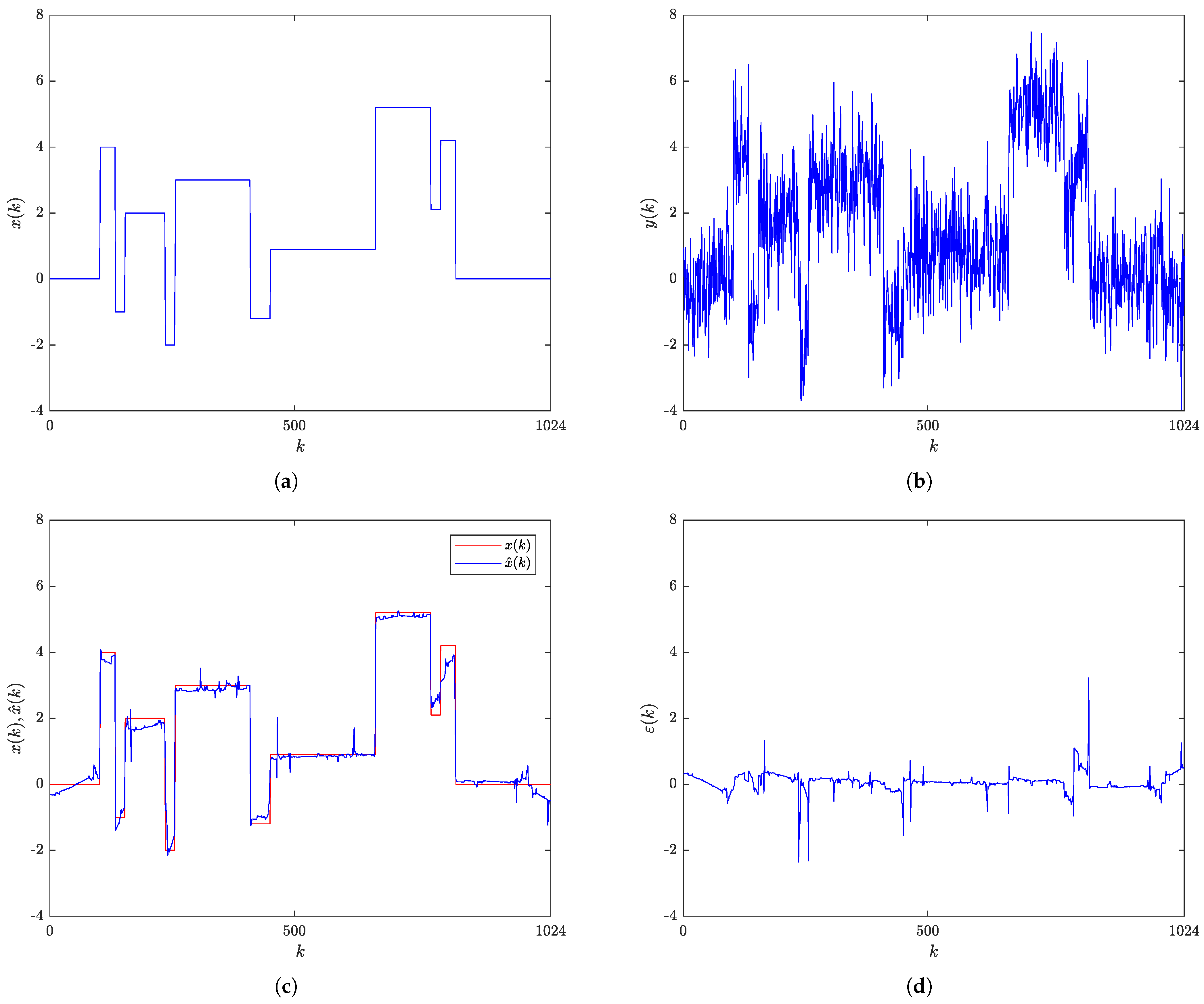
3.1.1. Blocks Signal

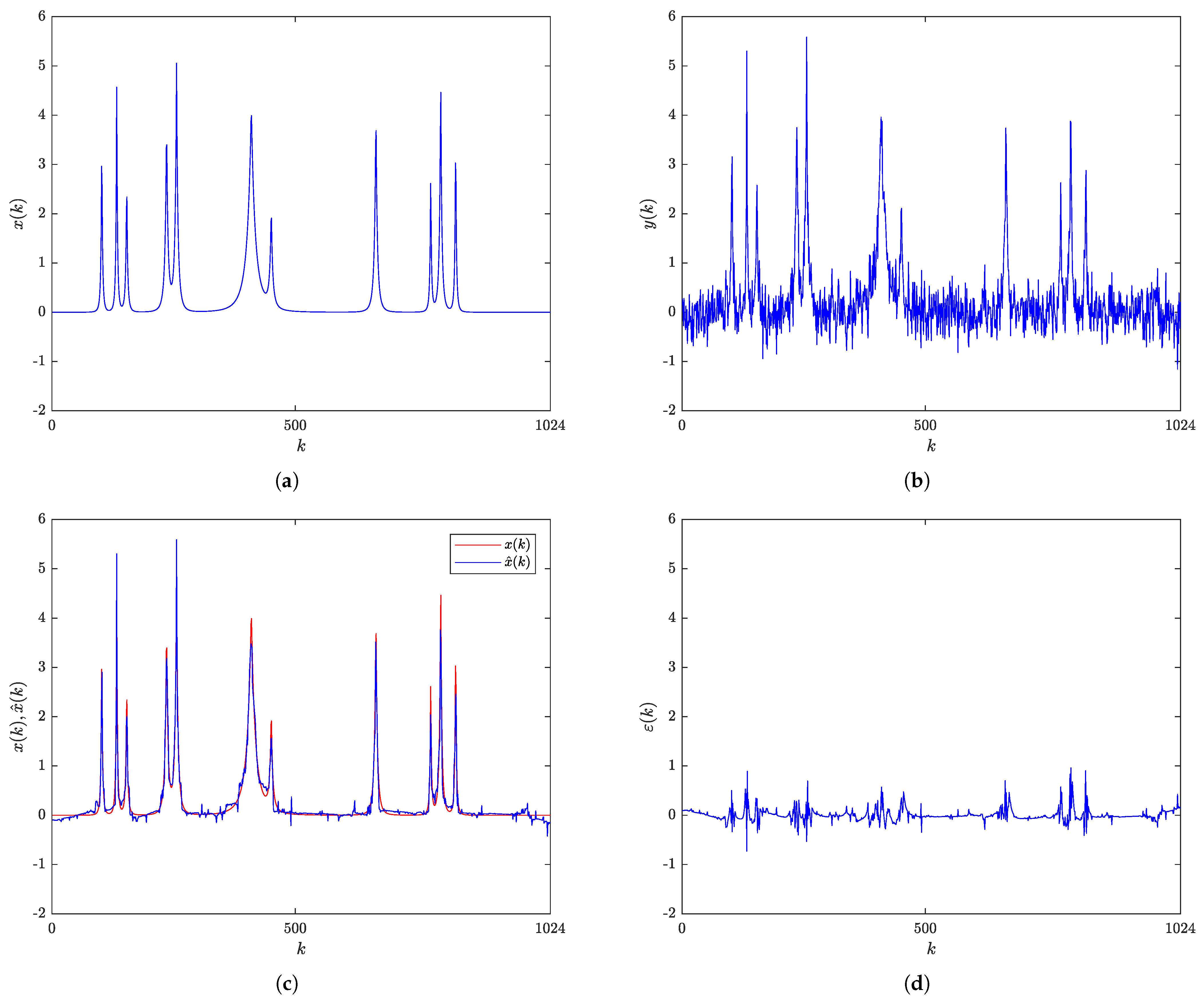
The original Blocks signal is shown in Figure 1a, while Figure 1b shows its noisy version, with the SNR of 7 dB. The results obtained by applying the RBF-RICI filtering algorithm, in terms of comparison of the original and the filtered signal, are presented in Figure 1c, while Figure 1d shows the filtering error. As can be seen, the RBF-RICI algorithm reduces the noise and reconstructs the main features of the original Blocks signal well, with the slightly degraded performance near the instantaneous signal value changes.

Figure 1. Blocks signal: (a) Original signal. (b) Noisy signal (SNR = 7 dB). (c) Original and RBF-RICI filtered signal ($\Gamma =1.44,R_c=0.67$). (d) Filtering error.

The filtering results obtained by the RBF-RICI, the LPA-RICI, the LPA-ICI, and the Savitzky–Golay filtering algorithm applied to the noisy Blocks signal at SNRs of 5, 7, and 10 dB are given in Table 1, Table 2 and Table 3, respectively. The quantitative comparison is provided by calculating the filtering quality indicators MSE, MAE, MAXE, PSNR, and ISNR for the tested algorithms with the optimal parameters, i.e., the parameters that minimize the filtering MSE. The best filtering quality indicators in each table, i.e., the lowest values of MSE, MAE, and MAXE, and the highest values of PSNR and ISNR, are marked in bold. The results presented in Table 1, Table 2 and Table 3 suggest that the RBF-RICI algorithm applied to the noisy Blocks signal provides satisfactory filtering performance, reducing the filtering errors and improving the SNR of the signal. With the decrease of the SNR, the RBF-RICI algorithm’s filtering quality is also somewhat reduced but remained competitive.

Table 1. Blocks signal (SNR = 5 dB)—Filtering results. The best filtering quality indicators are marked in bold.

Filtering Quality Indicator	RBF-RICI $\mathbf{\Gamma }=3.67$, ${\mathit{R}}_{\mathit{c}}=0.95$	LPA-RICI $\mathbf{\Gamma }=4.03$, ${\mathit{R}}_{\mathit{c}}=0.96$	LPA-ICI $\mathbf{\Gamma }=0.73$	Savitzky- Golay $\mathit{h}=25$
MSE	0.1409	0.1459	0.2114	0.3276
MAE	0.2132	0.2100	0.3264	0.4219
MAXE	3.6682	3.6471	4.0740	2.5848
PSNR (dB)	22.8307	22.6801	21.0700	19.1668
ISNR (dB)	11.4673	11.3166	9.7065	7.8033

Table 2. Blocks signal (SNR = 7 dB)—Filtering results.

Filtering Quality Indicator	RBF-RICI $\mathbf{\Gamma }=1.44$, ${\mathit{R}}_{\mathit{c}}=0.67$	LPA-RICI $\mathbf{\Gamma }=4.12$, ${\mathit{R}}_{\mathit{c}}=0.98$	LPA-ICI $\mathbf{\Gamma }=0.62$	Savitzky- Golay $\mathit{h}=21$
MSE	0.0849	0.0973	0.1305	0.2599
MAE	0.1797	0.1864	0.2550	0.3684
MAXE	3.2267	2.8130	2.9652	2.3588
PSNR (dB)	25.0323	24.4376	23.1630	20.1717
ISNR (dB)	11.6688	11.0741	9.7996	6.8082

Table 3. Blocks signal (SNR = 10 dB)—Filtering results.

Filtering Quality Indicator	RBF-RICI $\mathbf{\Gamma }=1.60$, ${\mathit{R}}_{\mathit{c}}=0.84$	LPA-RICI $\mathbf{\Gamma }=1.56$, ${\mathit{R}}_{\mathit{c}}=0.89$	LPA-ICI $\mathbf{\Gamma }=0.47$	Savitzky- Golay $\mathit{h}=19$
MSE	0.0311	0.0298	0.0595	0.1889
MAE	0.1000	0.1059	0.1703	0.2939
MAXE	2.4207	2.4023	2.4001	2.3602
PSNR (dB)	29.3877	29.5756	26.5776	21.5585
ISNR (dB)	13.0243	13.2121	10.2142	5.1951

The filtering quality improvement of the RBF-RICI algorithm over the other tested algorithms for the Blocks signal is calculated, and the percentage values are given in Table 4, Table 5 and Table 6 for SNRs of 5, 7, and 10 dB, respectively. The positive percentage values indicate the filtering quality improvement of the RBF-RICI algorithm over the other algorithms, i.e., the decrease in the values of the filtering quality indicators MSE, MAE, and MAXE, and the increase in the values of the PSNR and ISNR, while the negative percentage values indicate the opposite. The results provided in Table 4, Table 5 and Table 6 suggest that, in most cases, the RBF-RICI algorithm applied to the noisy Blocks signal provides the improved or competitive filtering quality when compared to the other tested algorithms.

Table 4. Blocks signal (SNR = 5 dB)—Filtering quality improvement of the RBF-RICI-based filtering over other tested algorithms.

Filtering Quality Indicator	LPA-RICI $\mathbf{\Gamma }=4.03$, ${\mathit{R}}_{\mathit{c}}=0.96$	LPA-ICI $\mathbf{\Gamma }=0.73$	Savitzky- Golay $\mathit{h}=25$
MSE	3.43%	33.35%	56.99%
MAE	−1.52%	34.68%	49.47%
MAXE	−0.58%	9.96%	−41.91%
PSNR (dB)	0.66%	8.36%	19.12%
ISNR (dB)	1.33%	18.14%	46.95%

Table 5. Blocks signal (SNR = 7 dB)—Filtering quality improvement of the RBF-RICI-based filtering over other tested algorithms.

Filtering Quality Indicator	LPA-RICI $\mathbf{\Gamma }=4.12$, ${\mathit{R}}_{\mathit{c}}=0.98$	LPA-ICI $\mathbf{\Gamma }=0.62$	Savitzky- Golay $\mathit{h}=21$
MSE	12.74%	34.94%	67.33%
MAE	3.59%	29.53%	51.22%
MAXE	−14.71%	−8.82%	−36.79%
PSNR (dB)	2.43%	8.07%	24.10%
ISNR (dB)	5.37%	19.07%	71.39%

Table 6. Blocks signal (SNR = 10 dB)—Filtering quality improvement of the RBF-RICI-based filtering over other tested algorithms.

Filtering Quality Indicator	LPA-RICI $\mathbf{\Gamma }=1.56$, ${\mathit{R}}_{\mathit{c}}=0.89$	LPA-ICI $\mathbf{\Gamma }=0.47$	Savitzky- Golay $\mathit{h}=19$
MSE	−4.36%	47.73%	83.54%
MAE	5.57%	41.28%	65.97%
MAXE	−0.77%	−0.86%	−2.56%
PSNR (dB)	−0.64%	10.57%	36.32%
ISNR (dB)	−1.42%	27.51%	150.70%

The runtimes have also been computed for each tested filtering algorithm. The algorithm runtimes have been obtained on a computer with the Intel Xeon CPU E5-2620 v4 @ 2.10 GHz, and 128 GB of RAM. The results have been averaged over 1000 algorithm runs. The runtimes of the filtering algorithms applied to the noisy Blocks signal at SNRs of 5, 7, and 10 dB are shown in Table 7. The presented results suggest that the proposed RBF-RICI algorithm performs competitively to the LPA-RICI and LPA-ICI algorithms in terms of execution speed, with a dependence on the selected parameters’ values. However, Savitzky–Golay filtering algorithm provides significantly faster performance than the other tested algorithms.

Table 7. Blocks signal—Filtering algorithms’ runtimes.

Runtime (s)
SNR (dB)	RBF-RICI	LPA-RICI	LPA-ICI	Savitzky–Golay
5	0.1439	0.2301	0.1482	0.0006
7	0.2655	0.0839	0.1351	0.0004
10	0.2136	0.2353	0.1413	0.0010

3.1.2. Bumps Signal

Figure 2a shows the original Bumps signal, whose noise-corrupted version with the SNR of 7 dB is shown in Figure 2b. The comparison of the original and the RBF-RICI filtered Bumps signal is given in Figure 2c, with the filtering error shown in Figure 2d. As shown in Figure 2c, the RBF-RICI algorithm provides very good noise reduction performance.

Figure 2. Bumps signal: (a) Original signal. (b) Noisy signal (SNR = 7 dB). (c) Original and RBF-RICI filtered signal ($\Gamma =0.82,R_c=0.33$). (d) Filtering error.

Table 8, Table 9 and Table 10 provide the filtering quality indicators obtained by the optimized RBF-RICI, LPA-RICI, LPA-ICI, and Savitzky–Golay filtering algorithms applied to the noisy Bumps signal for SNRs of 5, 7, and 10 dB, respectively. The results indicate that the RBF-RICI algorithm provides good filtering performance in terms of noise suppression and filtering error reduction. As expected, the filtering performance slightly declines with the decreasing SNR. Table 11, Table 12 and Table 13 give the relative comparison of the filtering quality obtained by the RBF-RICI algorithm and the other tested algorithms applied to the Bumps signal at SNRs of 5, 7, and 10 dB, respectively. The presented comparison indicates that the proposed RBF-RICI algorithm provides better performance than all other tested algorithms for each considered filtering quality indicator and SNR value.

Table 8. Bumps signal (SNR = 5 dB)—Filtering results.

Filtering Quality Indicator	RBF-RICI $\mathbf{\Gamma }=1.13$, ${\mathit{R}}_{\mathit{c}}=0.49$	LPA-RICI $\mathbf{\Gamma }=2.05$, ${\mathit{R}}_{\mathit{c}}=0.90$	LPA-ICI $\mathbf{\Gamma }=0.57$	Savitzky- Golay $\mathit{h}=9$
MSE	0.0277	0.0356	0.0382	0.0626
MAE	0.0966	0.1093	0.1215	0.1880
MAXE	1.1582	1.2638	1.2638	1.7304
PSNR (dB)	29.6493	28.5563	28.2463	26.1023
ISNR (dB)	7.8378	6.7449	6.4348	4.2909

Table 9. Bumps signal (SNR = 7 dB)—Filtering results.

Filtering Quality Indicator	RBF-RICI $\mathbf{\Gamma }=0.82$, ${\mathit{R}}_{\mathit{c}}=0.33$	LPA-RICI $\mathbf{\Gamma }=1.57$, ${\mathit{R}}_{\mathit{c}}=0.88$	LPA-ICI $\mathbf{\Gamma }=0.48$	Savitzky- Golay $\mathit{h}=9$
MSE	0.0181	0.0251	0.0279	0.0454
MAE	0.0806	0.0944	0.1028	0.1546
MAXE	0.9612	1.0178	1.0178	1.7418
PSNR (dB)	31.4981	30.0755	29.6152	27.4996
ISNR (dB)	7.6866	6.2640	5.8038	3.6881

Table 10. Bumps signal (SNR = 10 dB)—Filtering results.

Filtering Quality Indicator	RBF-RICI $\mathbf{\Gamma }=0.61$, ${\mathit{R}}_{\mathit{c}}=0.26$	LPA-RICI $\mathbf{\Gamma }=1.55$, ${\mathit{R}}_{\mathit{c}}=0.96$	LPA-ICI $\mathbf{\Gamma }=0.34$	Savitzky- Golay $\mathit{h}=7$
MSE	0.0101	0.0148	0.0166	0.0276
MAE	0.0599	0.0777	0.0790	0.1228
MAXE	0.7072	0.7327	0.8098	1.3599
PSNR (dB)	34.0275	32.3577	31.8621	29.6602
ISNR (dB)	7.2161	5.5462	5.0506	2.8487

Table 11. Bumps signal (SNR = 5 dB)—Filtering quality improvement of the RBF-RICI-based filtering over other tested algorithms.

Filtering Quality Indicator	LPA-RICI $\mathbf{\Gamma }=2.05$, ${\mathit{R}}_{\mathit{c}}=0.90$	LPA-ICI $\mathbf{\Gamma }=0.57$	Savitzky- Golay $\mathit{h}=9$
MSE	22.19%	27.49%	55.75%
MAE	11.62%	20.49%	48.62%
MAXE	8.36%	8.36%	33.07%
PSNR (dB)	3.83%	4.97%	13.59%
ISNR (dB)	16.20%	21.80%	82.66%

Table 12. Bumps signal (SNR = 7 dB)—Filtering quality improvement of the RBF-RICI-based filtering over other tested algorithms.

Filtering Quality Indicator	LPA-RICI $\mathbf{\Gamma }=1.57$, ${\mathit{R}}_{\mathit{c}}=0.88$	LPA-ICI $\mathbf{\Gamma }=0.48$	Savitzky- Golay $\mathit{h}=9$
MSE	27.89%	35.13%	60.13%
MAE	14.62%	21.60%	47.87%
MAXE	5.56%	5.56%	44.82%
PSNR (dB)	4.73%	6.36%	14.54%
ISNR (dB)	22.71%	32.44%	108.42%

Table 13. Bumps signal (SNR = 10 dB)—Filtering quality improvement of the RBF-RICI-based filtering over other tested algorithms.

Filtering Quality Indicator	LPA-RICI $\mathbf{\Gamma }=1.55$, ${\mathit{R}}_{\mathit{c}}=0.96$	LPA-ICI $\mathbf{\Gamma }=0.34$	Savitzky- Golay $\mathit{h}=7$
MSE	31.76%	39.16%	63.41%
MAE	22.91%	24.18%	51.22%
MAXE	3.48%	12.67%	48.00%
PSNR (dB)	5.16%	6.80%	14.72%
ISNR (dB)	30.11%	42.88%	153.31%

The filtering algorithms’ runtimes in the case of the Bumps signal filtered at SNR levels of 5, 7, and 10 dB are given in Table 14. The RBF-RICI algorithm shows performance that is significantly slower than the one obtained by the Savitzky–Golay filtering and somewhat slower than those provided by the LPA-RICI and LPA-ICI algorithms.

Table 14. Bumps signal—Filtering algorithms’ runtimes.

Runtime (s)
SNR (dB)	RBF-RICI	LPA-RICI	LPA-ICI	Savitzky-Golay
5	0.1740	0.1614	0.1117	0.0002
7	0.1974	0.1206	0.0937	0.0001
10	0.1812	0.0742	0.0845	0.0001

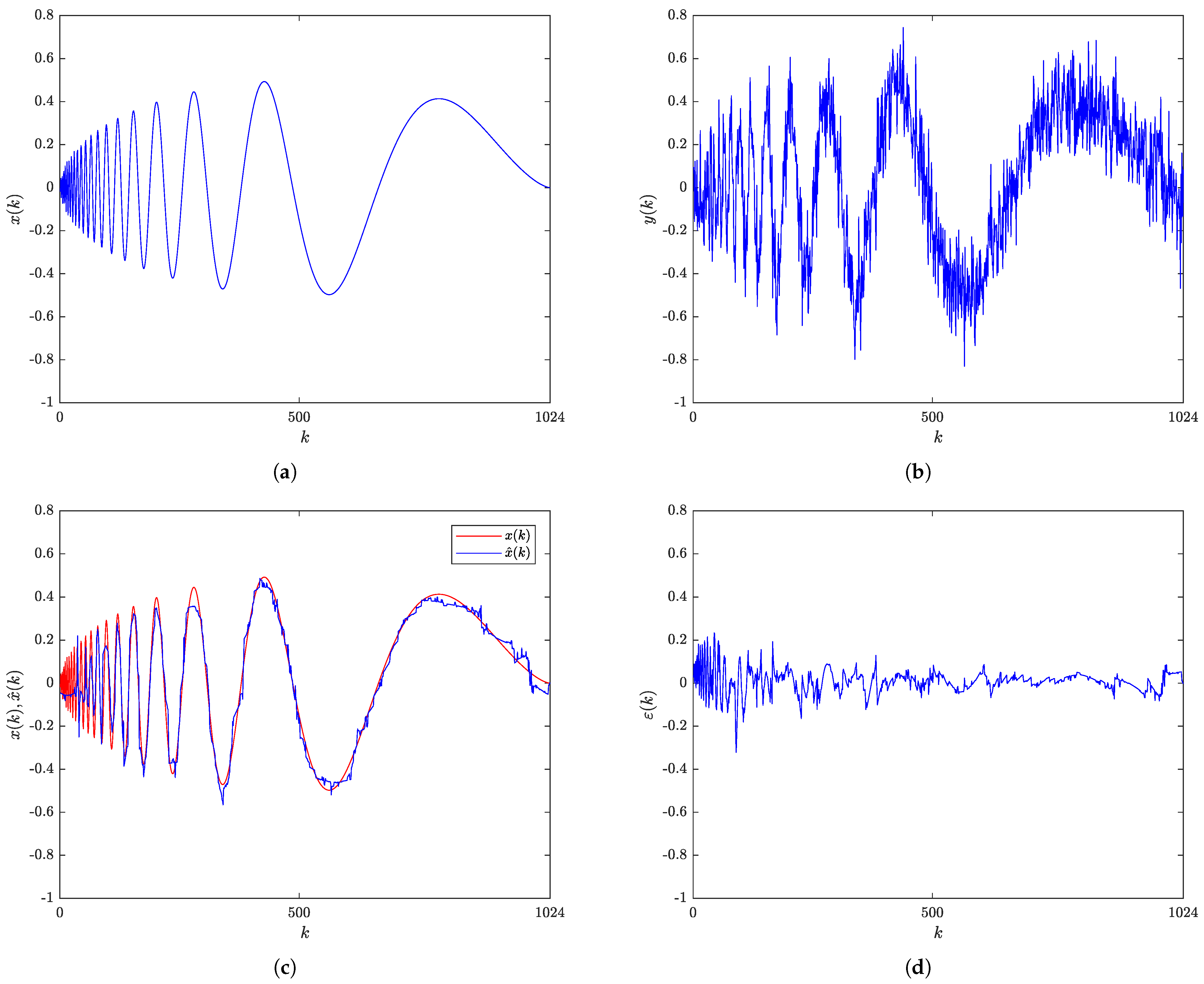
3.1.3. Doppler Signal

The original and noisy (SNR = 7 dB) Doppler signals are shown in Figure 3a,b, respectively. Figure 3c shows the original and the RBF-RICI filtered Doppler signal, while the obtained filtering error is shown in Figure 3d. As shown in Figure 3c, the RBF-RICI algorithm provides somewhat poorer filtering performance in the initial part of the Doppler signal where the higher frequency oscillations are present, and the algorithm’s performance significantly improves in the rest of the signal with the lower frequency content (and higher amplitudes).

Figure 3. Doppler signal: (a) Original signal. (b) Noisy signal (SNR = 7 dB). (c) Original and RBF-RICI filtered signal ($\Gamma =2.29,R_c=0.94$). (d) Filtering error.

The results obtained by applying the improved filtering algorithm to the noisy Doppler signal are given in Table 15, Table 16 and Table 17 for SNRs of 5, 7, and 10 dB, respectively. According to the values of the filtering quality indicators, the RBF-RICI technique provides a good filtering performance by reducing the filtering error and increasing the SNR of the signal. The percentage values describing the relative filtering quality improvement of the RBF-RICI algorithm over the LPA-RICI, the LPA-ICI, and the Savitzky–Golay filtering algorithm applied to the Doppler signal at SNRs of 5, 7, and 10 dB are given in Table 18, Table 19 and Table 20, respectively. The RBF-RICI algorithm outperforms all other tested algorithms for all filtering quality indicators and SNR values, except for the MAXE at the 7 dB SNR.

Table 15. Doppler signal (SNR = 5 dB)—Filtering results.

Filtering Quality Indicator	RBF-RICI $\mathbf{\Gamma }=2.15$, ${\mathit{R}}_{\mathit{c}}=0.88$	LPA-RICI $\mathbf{\Gamma }=4.82$, ${\mathit{R}}_{\mathit{c}}=1$	LPA-ICI $\mathbf{\Gamma }=0.58$	Savitzky- Golay $\mathit{h}=23$
MSE	0.0037	0.0046	0.0059	0.0044
MAE	0.0452	0.0496	0.0590	0.0481
MAXE	0.2647	0.3061	0.3028	0.2949
PSNR (dB)	18.2042	17.1874	16.1235	17.4454
ISNR (dB)	8.8026	7.7858	6.7220	8.0439

Table 16. Doppler signal (SNR = 7 dB)—Filtering results.

Filtering Quality Indicator	RBF-RICI $\mathbf{\Gamma }=2.29$, ${\mathit{R}}_{\mathit{c}}=0.94$	LPA-RICI $\mathbf{\Gamma }=3.61$, ${\mathit{R}}_{\mathit{c}}=1$	LPA-ICI $\mathbf{\Gamma }=0.46$	Savitzky- Golay $\mathit{h}=21$
MSE	0.0027	0.0033	0.0045	0.0034
MAE	0.0373	0.0417	0.0512	0.0412
MAXE	0.3212	0.2803	0.3177	0.2776
PSNR (dB)	19.5106	18.6596	17.3110	18.5490
ISNR (dB)	8.1091	7.2581	5.9094	7.1475

Table 17. Doppler signal (SNR = 10 dB)—Filtering results.

Filtering Quality Indicator	RBF-RICI $\mathbf{\Gamma }=2.85$, ${\mathit{R}}_{\mathit{c}}=1$	LPA-RICI $\mathbf{\Gamma }=2.55$, ${\mathit{R}}_{\mathit{c}}=1$	LPA-ICI $\mathbf{\Gamma }=0.35$	Savitzky- Golay $\mathit{h}=17$
MSE	0.0017	0.0021	0.0030	0.0023
MAE	0.0293	0.0319	0.0411	0.0332
MAXE	0.2097	0.2553	0.2809	0.2643
PSNR (dB)	21.5377	20.6978	19.1250	20.2577
ISNR (dB)	7.1362	6.2962	4.7235	5.8561

Table 18. Doppler signal (SNR = 5 dB)—Filtering quality improvement of the RBF-RICI-based filtering over other tested algorithms.

Filtering Quality Indicator	LPA-RICI $\mathbf{\Gamma }=4.82$, ${\mathit{R}}_{\mathit{c}}=1$	LPA-ICI $\mathbf{\Gamma }=0.58$	Savitzky- Golay $\mathit{h}=23$
MSE	19.57%	37.29%	15.91%
MAE	8.87%	23.39%	6.03%
MAXE	13.52%	12.58%	10.24%
PSNR (dB)	5.92%	12.90%	4.35%
ISNR (dB)	13.06%	30.95%	9.43%

Table 19. Doppler signal (SNR = 7 dB)—Filtering quality improvement of the RBF-RICI-based filtering over other tested algorithms.

Filtering Quality Indicator	LPA-RICI $\mathbf{\Gamma }=3.61$, ${\mathit{R}}_{\mathit{c}}=1$	LPA-ICI $\mathbf{\Gamma }=0.46$	Savitzky- Golay $\mathit{h}=21$
MSE	18.18%	40.00%	20.59%
MAE	10.55%	27.15%	9.47%
MAXE	−14.59%	−1.10%	−15.71%
PSNR (dB)	4.56%	12.71%	5.18%
ISNR (dB)	11.72%	37.22%	13.45%

Table 20. Doppler signal (SNR = 10 dB)—Filtering quality improvement of the RBF-RICI-based filtering over other tested algorithms.

Filtering Quality Indicator	LPA-RICI $\mathbf{\Gamma }=2.55$, ${\mathit{R}}_{\mathit{c}}=1$	LPA-ICI $\mathbf{\Gamma }=0.35$	Savitzky- Golay $\mathit{h}=17$
MSE	19.05%	43.33%	26.09%
MAE	8.15%	28.71%	11.75%
MAXE	17.86%	25.35%	20.66%
PSNR (dB)	4.06%	12.62%	6.32%
ISNR (dB)	13.34%	51.08%	21.86%

The runtimes calculated for the filtering algorithms applied to the Doppler signal at SNRs of 5, 7, and 10 dB are given in Table 21. The RBF-RICI algorithm provides the runtimes which are competitive to the ones obtained by the LPA-RICI and LPA-ICI algorithms, with a dependence on the SNR and parameters’ values. These algorithms are again outperformed by the Savitzky–Golay filtering in terms of execution speed.

Table 21. Doppler signal—Filtering algorithms’ runtimes.

Runtime (s)
SNR (dB)	RBF-RICI	LPA-RICI	LPA-ICI	Savitzky–Golay
5	0.1600	0.0658	0.0947	0.0010
7	0.1177	0.0464	0.0836	0.0004
10	0.0512	0.0555	0.0702	0.0007

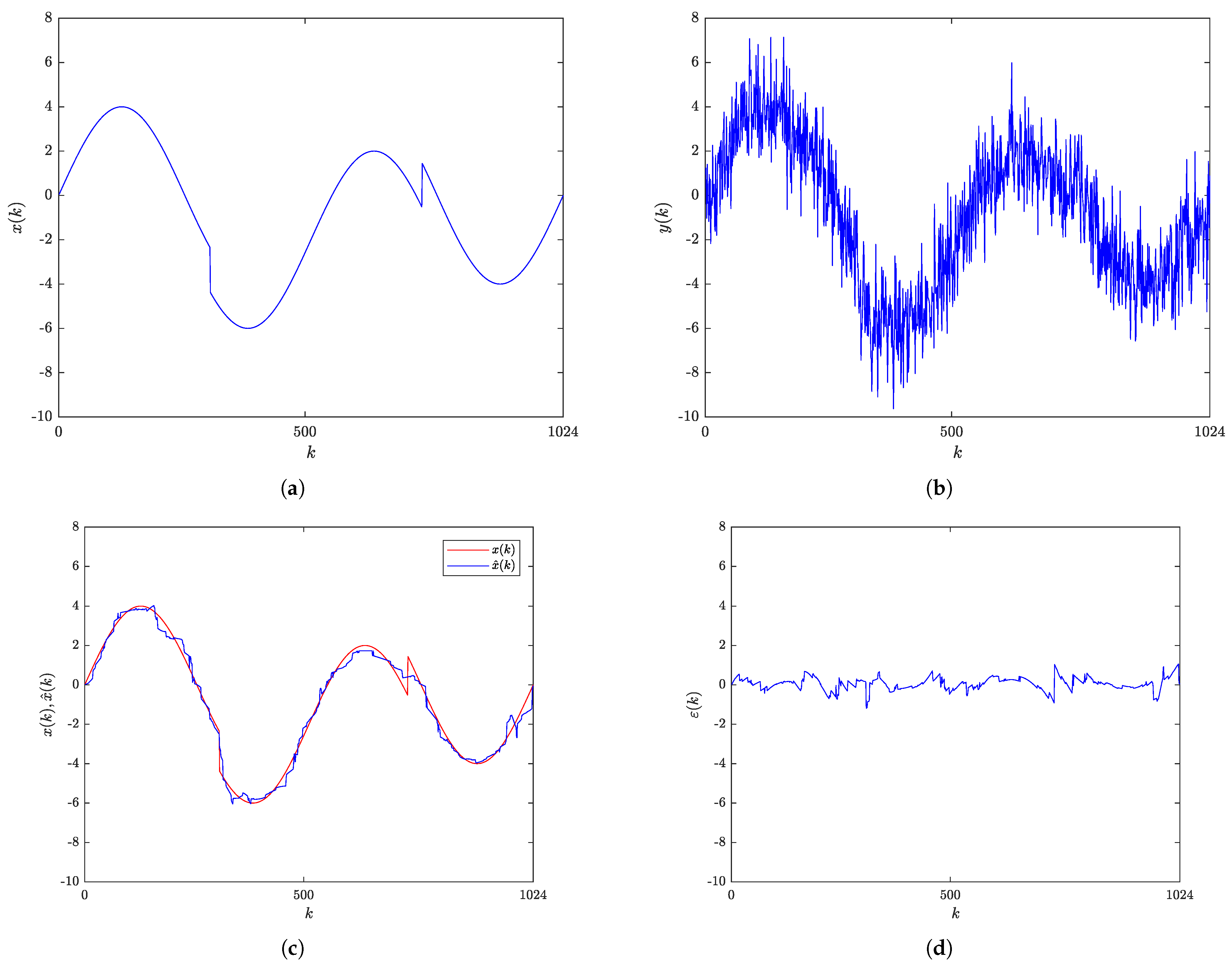
3.1.4. HeaviSine Signal

Figure 4a shows the original noise-free HeaviSine signal, while Figure 4b shows its noise-corrupted version at the 7 dB SNR. The comparison between the original and the RBF-RICI filtered signal is given in Figure 4c, while their difference is illustrated in Figure 4d as the filtering error. The proposed filtering algorithm provides noise reduction and estimates the original signal efficiently, with the low values of filtering error for the whole signal duration. The signal value jump at $k=307$ is successfully reconstructed, in contrast to the sudden change in the signal value at $k=737$ where the algorithm did not adapt fast enough.

Figure 4. HeaviSine signal: (a) Original signal. (b) Noisy signal (SNR = 7 dB). (c) Original and RBF-RICI filtered signal ($\Gamma =4.98,R_c=0.99$). (d) Filtering error.

Table 22, Table 23 and Table 24 provide the filtering results for the RBF-RICI, the LPA-RICI, the LPA-ICI, and the Savitzky–Golay filtering algorithm in the case of the HeaviSine signal filtered at SNRs of 5, 7, and 10 dB, respectively. The obtained filtering quality indicators suggest that the RBF-RICI algorithm efficiently removes the noise, keeping the filtering error at low values. The filtering quality is somewhat reduced for the lower SNR values but remained satisfactory. Table 25, Table 26 and Table 27 give the comparison between the filtering quality indicators obtained by the algorithms applied to the HeaviSine signal at SNRs of 5, 7, and 10 dB, respectively. The RBF-RICI algorithm shows better filtering performance than the LPA-RICI and LPA-ICI algorithms for each SNR case, but it is outperformed by the Savitzky–Golay filtering algorithm.

Table 22. HeaviSine signal (SNR = 5 dB)—Filtering results.

Filtering Quality Indicator	RBF-RICI $\mathbf{\Gamma }=4.98$, ${\mathit{R}}_{\mathit{c}}=0.98$	LPA-RICI $\mathbf{\Gamma }=4.97$, ${\mathit{R}}_{\mathit{c}}=0.99$	LPA-ICI $\mathbf{\Gamma }=0.61$	Savitzky- Golay $\mathit{h}=217$
MSE	0.1683	0.2022	0.3517	0.0995
MAE	0.3264	0.3432	0.4737	0.2217
MAXE	1.2817	1.8795	2.7010	1.0594
PSNR (dB)	19.7793	18.9828	16.5791	22.0611
ISNR (dB)	12.6436	11.8471	9.4434	14.9254

Table 23. HeaviSine signal (SNR = 7 dB)—Filtering results.

Filtering Quality Indicator	RBF-RICI $\mathbf{\Gamma }=4.98$, ${\mathit{R}}_{\mathit{c}}=0.99$	LPA-RICI $\mathbf{\Gamma }=4.54$, ${\mathit{R}}_{\mathit{c}}=0.99$	LPA-ICI $\mathbf{\Gamma }=0.51$	Savitzky- Golay $\mathit{h}=101$
MSE	0.1070	0.1280	0.2540	0.0763
MAE	0.2526	0.2763	0.3987	0.2001
MAXE	1.1832	1.8756	2.6166	1.0451
PSNR (dB)	21.7477	20.9676	17.9928	23.2185
ISNR (dB)	12.6119	11.8319	8.8571	14.0828

Table 24. HeaviSine signal (SNR = 10 dB)—Filtering results.

Filtering Quality Indicator	RBF-RICI $\mathbf{\Gamma }=4.85$, ${\mathit{R}}_{\mathit{c}}=1$	LPA-RICI $\mathbf{\Gamma }=4.67$, ${\mathit{R}}_{\mathit{c}}=1$	LPA-ICI $\mathbf{\Gamma }=0.38$	Savitzky- Golay $\mathit{h}=101$
MSE	0.0594	0.0668	0.1549	0.0536
MAE	0.1782	0.1924	0.3101	0.1578
MAXE	1.0415	0.9900	2.4188	1.0251
PSNR (dB)	24.3045	23.7948	20.1394	24.7476
ISNR (dB)	12.1688	11.6591	8.0037	12.6118

Table 25. HeaviSine signal (SNR = 5 dB)—Filtering quality improvement of the RBF-RICI-based filtering over other tested algorithms.

Filtering Quality Indicator	LPA-RICI $\mathbf{\Gamma }=4.97$, ${\mathit{R}}_{\mathit{c}}=0.99$	LPA-ICI $\mathbf{\Gamma }=0.61$	Savitzky- Golay $\mathit{h}=217$
MSE	16.77%	52.15%	−69.15%
MAE	4.90%	31.10%	−47.23%
MAXE	31.81%	52.55%	−20.98%
PSNR (dB)	4.20%	19.30%	−10.34%
ISNR (dB)	6.72%	33.89%	−15.29%

Table 26. HeaviSine signal (SNR = 7 dB)—Filtering quality improvement of the RBF-RICI-based filtering over other tested algorithms.

Filtering Quality Indicator	LPA-RICI $\mathbf{\Gamma }=4.54$, ${\mathit{R}}_{\mathit{c}}=0.99$	LPA-ICI $\mathbf{\Gamma }=0.51$	Savitzky- Golay $\mathit{h}=101$
MSE	16.41%	57.87%	−40.24%
MAE	8.58%	36.64%	−26.24%
MAXE	36.92%	54.78%	−13.21%
PSNR (dB)	3.72%	20.87%	−6.33%
ISNR (dB)	6.59%	42.39%	−10.44%

Table 27. HeaviSine signal (SNR = 10 dB)—Filtering quality improvement of the RBF-RICI-based filtering over other tested algorithms.

Filtering Quality Indicator	LPA-RICI $\mathbf{\Gamma }=4.67$, ${\mathit{R}}_{\mathit{c}}=1$	LPA-ICI $\mathbf{\Gamma }=0.38$	Savitzky- Golay $\mathit{h}=101$
MSE	11.08%	61.65%	−10.82%
MAE	7.38%	42.53%	−12.93%
MAXE	−5.20%	56.94%	−1.60%
PSNR (dB)	2.14%	20.68%	−1.79%
ISNR (dB)	4.37%	52.04%	−3.51%

The filtering algorithms’ runtimes for the noisy HeaviSine signal considered at SNR levels of 5, 7, and 10 dB are shown in Table 28. The RBF-RICI algorithm is competitive to the LPA-RICI and LPA-ICI algorithms in terms of execution speed, outperforming both methods at the SNR of 10 dB. The Savitzky–Golay filtering provides the fastest performance.

Table 28. HeaviSine signal—Filtering algorithms’ runtimes.

Runtime (s)
SNR (dB)	RBF-RICI	LPA-RICI	LPA-ICI	Savitzky–Golay
5	0.2017	0.1275	0.1274	0.0010
7	0.1428	0.1061	0.1534	0.0009
10	0.0942	0.1177	0.1102	0.0015

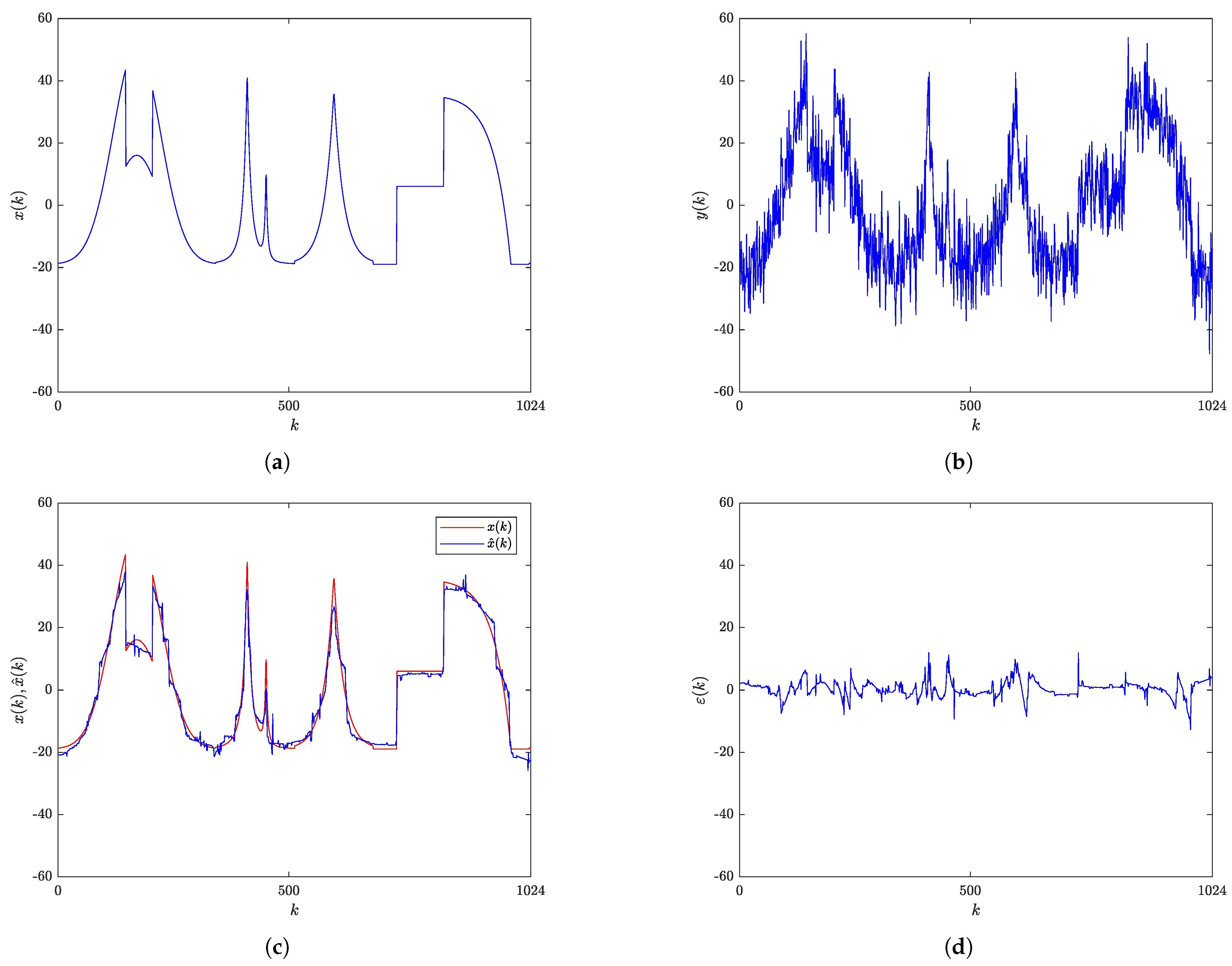
3.1.5. Piece-Regular Signal

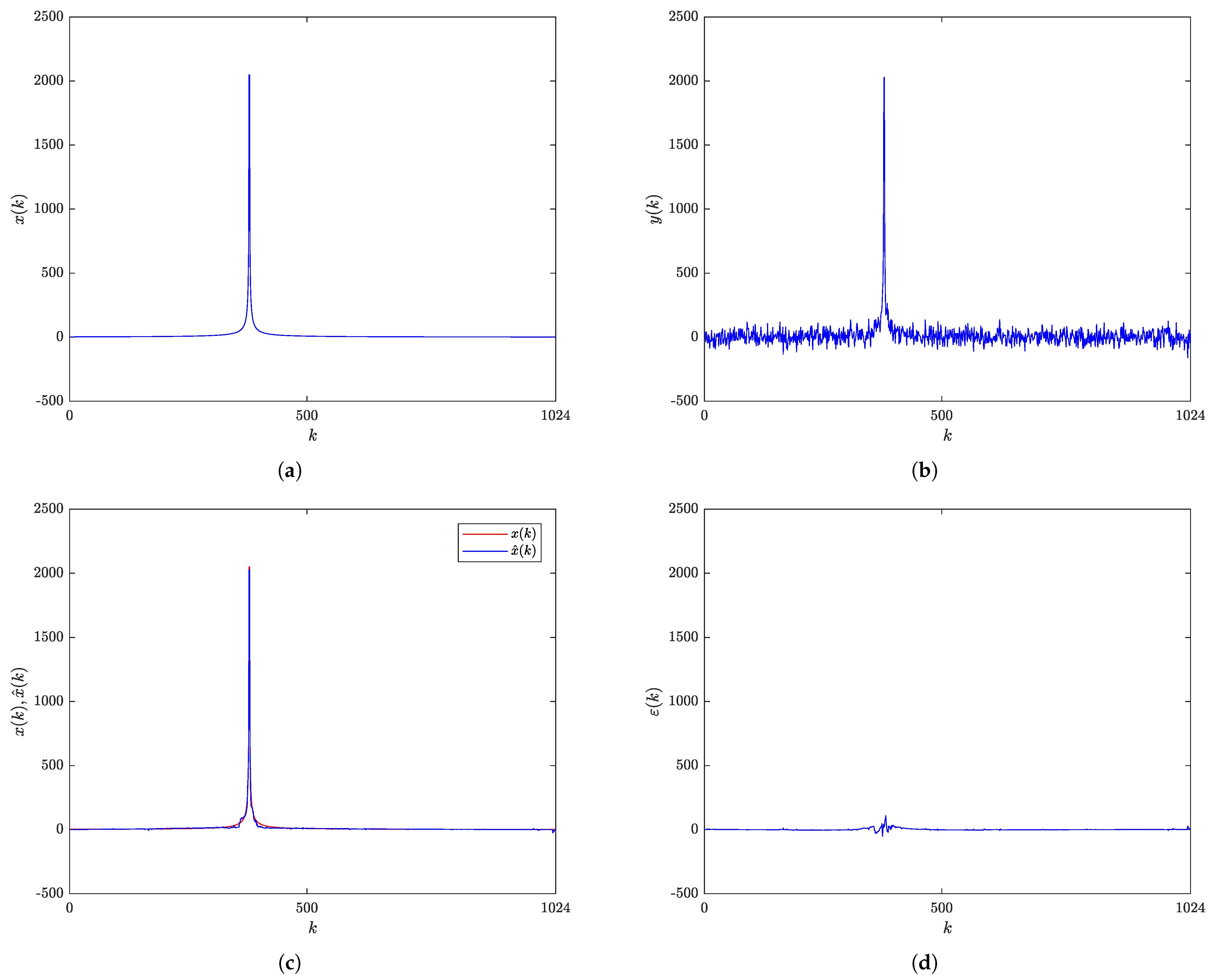
Figure 5a,b show the original and the noisy (SNR = 7 dB) Piece-Regular signal, respectively. The original and the RBF-RICI filtered signals are shown in Figure 5c, while Figure 5d shows the obtained estimation error. The results presented in Figure 5c,d suggest that the proposed adaptive algorithm provides excellent filtering accuracy, as the original signal and the filtered signal match closely. The algorithm adapts well to all sudden changes in signal slope and value.

Figure 5. Piece-Regular signal: (a) Original signal. (b) Noisy signal (SNR = 7 dB). (c) Original and RBF-RICI filtered signal ($\Gamma =1.44,R_c=0.81$). (d) Filtering error.

The results presented in Table 29, Table 30 and Table 31 suggest that the proposed RBF-RICI algorithm applied to the noisy Piece-Regular signal provides excellent filtering performance. The performance deteriorates somewhat with decreasing SNR. As shown in Table 32, Table 33 and Table 34, the RBF-RICI algorithm outperforms all other tested algorithms applied to the Piece-Regular signal for each considered SNR.

Table 29. Piece-Regular signal (SNR = 5 dB)—Filtering results.

Filtering Quality Indicator	RBF-RICI $\mathbf{\Gamma }=1.72$, ${\mathit{R}}_{\mathit{c}}=0.82$	LPA-RICI $\mathbf{\Gamma }=4.80$, ${\mathit{R}}_{\mathit{c}}=1$	LPA-ICI $\mathbf{\Gamma }=0.57$	Savitzky- Golay $\mathit{h}=25$
MSE	10.6693	14.1213	18.3593	13.3110
MAE	2.3735	2.7457	3.1596	2.7866
MAXE	17.7053	19.0331	18.5048	15.9277
PSNR (dB)	22.4826	21.2653	20.1255	21.5219
ISNR (dB)	9.9092	8.6918	7.5520	8.9485

Table 30. Piece-Regular signal (SNR = 7 dB)—Filtering results.

Filtering Quality Indicator	RBF-RICI $\mathbf{\Gamma }=1.44$, ${\mathit{R}}_{\mathit{c}}=0.81$	LPA-RICI $\mathbf{\Gamma }=3.77$, ${\mathit{R}}_{\mathit{c}}=1$	LPA-ICI $\mathbf{\Gamma }=0.47$	Savitzky- Golay $\mathit{h}=25$
MSE	7.0609	9.5441	13.0202	9.9522
MAE	1.9533	2.2509	2.6585	2.3151
MAXE	12.7040	18.3339	15.7328	15.2692
PSNR (dB)	24.2754	22.9667	21.6178	22.7848
ISNR (dB)	9.7020	8.3932	7.0444	8.2114

Table 31. Piece-Regular signal (SNR = 10 dB)—Filtering results.

Filtering Quality Indicator	RBF-RICI $\mathbf{\Gamma }=1.19$, ${\mathit{R}}_{\mathit{c}}=0.84$	LPA-RICI $\mathbf{\Gamma }=2.86$, ${\mathit{R}}_{\mathit{c}}=1$	LPA-ICI $\mathbf{\Gamma }=0.35$	Savitzky- Golay $\mathit{h}=19$
MSE	3.7850	5.2971	7.6770	6.7829
MAE	1.4513	1.6479	2.0257	1.8895
MAXE	8.7759	16.1955	12.8774	14.5437
PSNR (dB)	26.9834	25.5236	23.9121	24.4498
ISNR (dB)	9.4099	7.9502	6.3386	6.8764

Table 32. Piece-Regular signal (SNR = 5 dB)—Filtering quality improvement of the RBF-RICI-based filtering over other tested algorithms.

Filtering Quality Indicator	LPA-RICI $\mathbf{\Gamma }=4.80$, ${\mathit{R}}_{\mathit{c}}=1$	LPA-ICI $\mathbf{\Gamma }=0.57$	Savitzky- Golay $\mathit{h}=25$
MSE	24.45%	41.89%	19.85%
MAE	13.56%	24.88%	14.82%
MAXE	6.98%	4.32%	−11.16%
PSNR (dB)	5.72%	11.71%	4.46%
ISNR (dB)	14.01%	31.21%	10.74%

Table 33. Piece-Regular signal (SNR = 7 dB)—Filtering quality improvement of the RBF-RICI-based filtering over other tested algorithms.

Filtering Quality Indicator	LPA-RICI $\mathbf{\Gamma }=3.77$, ${\mathit{R}}_{\mathit{c}}=1$	LPA-ICI $\mathbf{\Gamma }=0.47$	Savitzky- Golay $\mathit{h}=25$
MSE	26.02%	45.77%	29.05%
MAE	13.22%	26.53%	15.63%
MAXE	30.71%	19.25%	16.80%
PSNR (dB)	5.70%	12.29%	6.54%
ISNR (dB)	15.59%	37.73%	18.15%

Table 34. Piece-Regular signal (SNR = 10 dB)—Filtering quality improvement of the RBF-RICI-based filtering over other tested algorithms.

Filtering Quality Indicator	LPA-RICI $\mathbf{\Gamma }=2.86$, ${\mathit{R}}_{\mathit{c}}=1$	LPA-ICI $\mathbf{\Gamma }=0.35$	Savitzky- Golay $\mathit{h}=19$
MSE	28.55%	50.70%	44.20%
MAE	11.93%	28.36%	23.19%
MAXE	45.81%	31.85%	39.66%
PSNR (dB)	5.72%	12.84%	10.36%
ISNR (dB)	18.36%	48.45%	36.84%

Table 35 gives the runtimes of the filtering algorithms applied to the noisy Piece-Regular signal at SNRs of 5, 7, and 10 dB. In this case, the RBF-RICI algorithm provides a slower performance when compared to the other tested algorithms.

Table 35. Piece-Regular signal—Filtering algorithms’ runtimes.

Runtime (s)
SNR (dB)	RBF-RICI	LPA-RICI	LPA-ICI	Savitzky–Golay
5	0.1522	0.0670	0.0862	0.0003
7	0.1459	0.0532	0.0975	0.0007
10	0.1366	0.0674	0.0873	0.0005

3.1.6. Sing Signal

The original Sing signal and the signal with the added white Gaussian noise (SNR = 7 dB) are shown in Figure 6a,b, respectively. The comparison between the original and the filtered signal is given in Figure 6c, with the filtering error shown in Figure 6d. The Sing signal is characterized by having zero values for the most part of its duration and one sudden peak of high amplitude, making it challenging for the filtering algorithm to adapt in a short period of time. The visual inspection of the presented results suggests that the optimized RBF-RICI algorithm provides excellent filtering performance with efficient noise suppression and an almost perfect match between the original and the filtered signal for the entire signal duration.

Figure 6. Sing signal: (a) Original signal. (b) Noisy signal (SNR = 7 dB). (c) Original and RBF-RICI filtered signal ($\Gamma =0.99,R_c=0.01$). (d) Filtering error.

Table 36, Table 37 and Table 38 provide the results obtained by the RBF-RICI, the LPA-RICI, the LPA-ICI, and the Savitzky–Golay filtering algorithm when applied to the filtering of the noisy Sing signal at SNRs of 5, 7, and 10 dB, respectively. The analysis of the calculated filtering quality indicators suggests that the RBF-RICI algorithm efficiently removes the noise, decreasing the filtering error and increasing the SNR of the signal. The performance is slightly reduced at the lower SNR values. The comparison of the filtering quality indicators obtained by the tested algorithms applied to the Sing signal, given in Table 39, Table 40 and Table 41, suggests that the RBF-RICI algorithm shows better filtering performance than the other tested algorithms for each filtering quality indicator and each considered SNR case.

Table 36. Sing signal (SNR = 5 dB)—Filtering results.

Filtering Quality Indicator	RBF-RICI $\mathbf{\Gamma }=1.12$, ${\mathit{R}}_{\mathit{c}}=0.11$	LPA-RICI $\mathbf{\Gamma }=2.81$, ${\mathit{R}}_{\mathit{c}}=0.94$	LPA-ICI $\mathbf{\Gamma }=0.82$	Savitzky- Golay $\mathit{h}=5$
MSE	83.8782	141.4546	177.6915	1962.6767
MAE	3.8877	6.4314	6.8539	33.8149
MAXE	111.5364	211.4573	193.0249	303.2041
PSNR (dB)	46.9901	44.7204	43.7299	33.2981
ISNR (dB)	15.9259	13.6562	12.6657	2.2339

Table 37. Sing signal (SNR = 7 dB)—Filtering results.

Filtering Quality Indicator	RBF-RICI $\mathbf{\Gamma }=0.99$, ${\mathit{R}}_{\mathit{c}}=0.01$	LPA-RICI $\mathbf{\Gamma }=1.87$, ${\mathit{R}}_{\mathit{c}}=0.91$	LPA-ICI $\mathbf{\Gamma }=0.73$	Savitzky- Golay $\mathit{h}=5$
MSE	64.1788	80.2616	132.0162	1338.2816
MAE	3.3283	5.4335	5.8075	27.0899
MAXE	108.9616	114.1618	171.9973	300.6734
PSNR (dB)	48.1527	47.1815	45.0203	34.9611
ISNR (dB)	15.0885	14.1173	11.9561	1.8969

Table 38. Sing signal (SNR = 10 dB)—Filtering results.

Filtering Quality Indicator	RBF-RICI $\mathbf{\Gamma }=0.68$, ${\mathit{R}}_{\mathit{c}}=0.11$	LPA-RICI $\mathbf{\Gamma }=2.11$, ${\mathit{R}}_{\mathit{c}}=0.96$	LPA-ICI $\mathbf{\Gamma }=0.44$	Savitzky- Golay $\mathit{h}=5$
MSE	35.3108	50.3365	73.5058	804.6591
MAE	2.4840	4.0478	4.7087	19.5046
MAXE	84.0245	99.7517	115.0057	297.8189
PSNR (dB)	50.7475	49.2078	47.5634	37.1705
ISNR (dB)	14.6833	13.1435	11.4992	1.1062

Table 39. Sing signal (SNR = 5 dB)—Filtering quality improvement of the RBF-RICI-based filtering over other tested algorithms.

Filtering Quality Indicator	LPA-RICI $\mathbf{\Gamma }=2.81$, ${\mathit{R}}_{\mathit{c}}=0.94$	LPA-ICI $\mathbf{\Gamma }=0.82$	Savitzky- Golay $\mathit{h}=5$
MSE	40.70%	52.80%	95.73%
MAE	39.55%	43.28%	88.50%
MAXE	47.25%	42.22%	63.21%
PSNR (dB)	5.08%	7.46%	41.12%
ISNR (dB)	16.62%	25.74%	612.93%

Table 40. Sing signal (SNR = 7 dB)—Filtering quality improvement of the RBF-RICI-based filtering over other tested algorithms.

Filtering Quality Indicator	LPA-RICI $\mathbf{\Gamma }=1.87$, ${\mathit{R}}_{\mathit{c}}=0.91$	LPA-ICI $\mathbf{\Gamma }=0.73$	Savitzky- Golay $\mathit{h}=5$
MSE	20.04%	51.39%	95.20%
MAE	38.74%	42.69%	87.71%
MAXE	4.56%	36.65%	63.76%
PSNR (dB)	2.06%	6.96%	37.73%
ISNR (dB)	6.88%	26.20%	695.43%

Table 41. Sing signal (SNR = 10 dB)—Filtering quality improvement of the RBF-RICI-based filtering over other tested algorithms.

Filtering Quality Indicator	LPA-RICI $\mathbf{\Gamma }=2.11$, ${\mathit{R}}_{\mathit{c}}=0.96$	LPA-ICI $\mathbf{\Gamma }=0.44$	Savitzky- Golay $\mathit{h}=5$
MSE	29.85%	51.96%	95.61%
MAE	38.63%	47.25%	87.26%
MAXE	15.77%	26.94%	71.79%
PSNR (dB)	3.13%	6.69%	36.53%
ISNR (dB)	11.72%	27.69%	1227.30%

Table 42 provides the filtering algorithms’ runtimes in the case of the noisy Sing signal filtered at SNR levels of 5, 7, and 10 dB. The results suggest that the RBF-RICI algorithm is outperformed by the other tested algorithms in terms of the execution speed.

Table 42. Sing signal—Filtering algorithms’ runtimes.

Runtime (s)
SNR (dB)	RBF-RICI	LPA-RICI	LPA-ICI	Savitzky-Golay
5	1.1708	0.9176	0.8507	0.0001
7	1.5391	0.4543	0.8060	0.0001
10	1.1189	0.7373	0.5872	0.0001

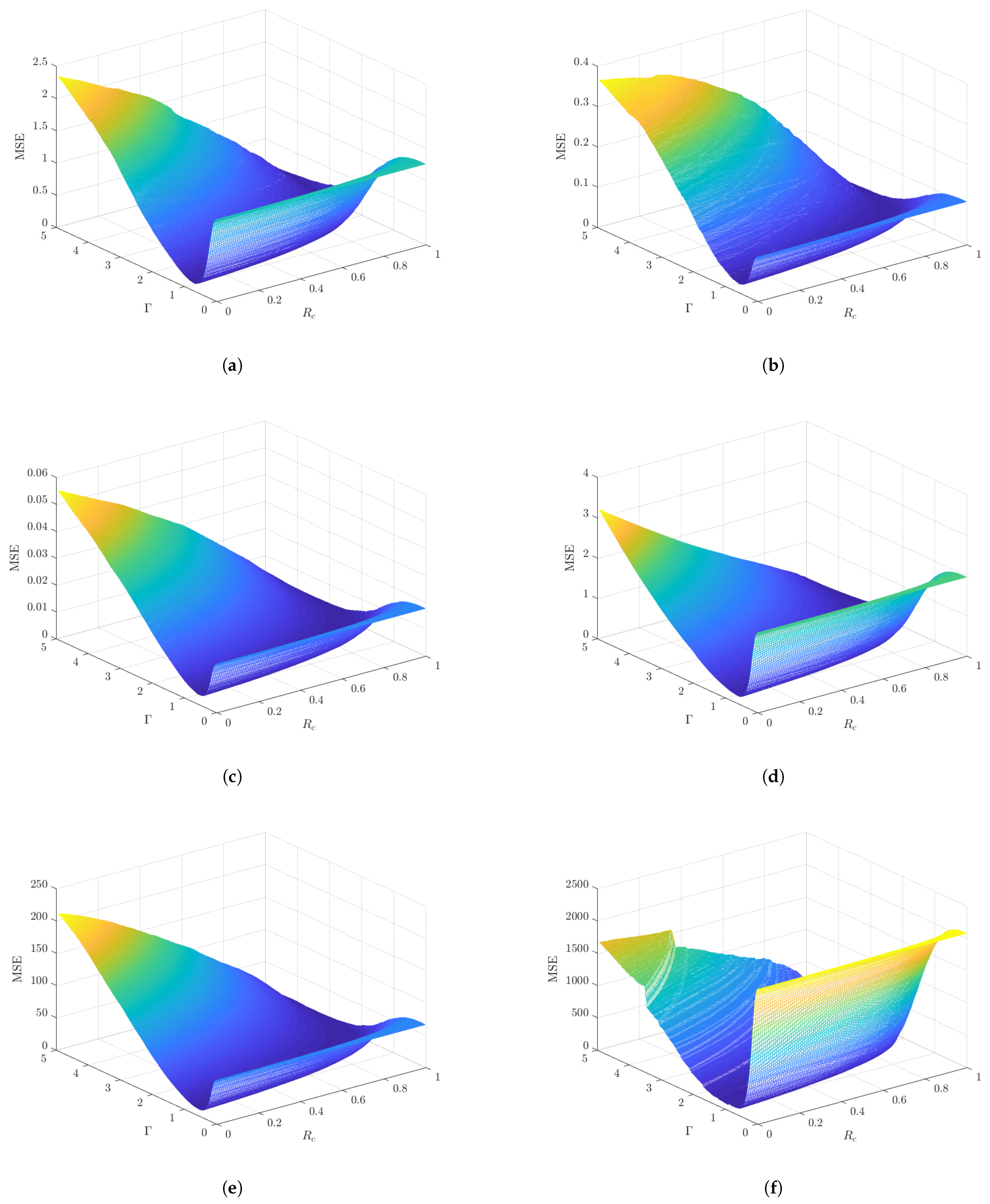
3.1.7. Parameters Sensitivity

In addition to the analysis provided above, Figure 7 shows the filtering quality measure MSE as a function of the RBF-RICI algorithm’s parameters $\Gamma$ and $R_c$, for the algorithm applied to each considered noisy signal at the SNR of 7 dB. The MSE values are calculated during the grid search in the parameter space, within the range $0\le \Gamma \le 5$ and $0\le R_c\le 1$. As can be seen, the estimation MSE, whose value determines the filtering performance, depends heavily on the proper selection of the algorithm’s parameters. In order to reduce the total number of evaluations needed to find the parameters’ values that minimize the obtained MSE, the parameters optimization approach following the PSO-based procedure is proposed.

Figure 7. The filtering quality indicator MSE as a function of the RBF-RICI algorithm’s parameters $\Gamma$ and $R_c$ for noisy signals at 7 dB SNR: (a) Blocks. (b) Bumps. (c) Doppler. (d) HeaviSine. (e) Piece-Regular. (f) Sing.

3.1.8. Effects of the Signal Length

The effects of the signal length on the RBF-RICI algorithm’s filtering performance are demonstrated on each considered test signal for the SNR of 7 dB. The obtained results are shown in Table 43. The RBF-RICI parameters are set to the values which are in the previous analysis found as optimal for each signal of the 1024 samples length. As can be seen in Table 43, the filtering performance is generally improved with the increasing signal length, i.e., the filtering errors are reduced, and the SNR is increased. The only exceptions are the MAXE which does not always show this declining trend, and the Sing signal due to its specific nature in which the high-amplitude and the narrow-width peak is not adequately registered at lower sampling rates. As expected, the algorithm runtime is increased for longer duration signals.

Table 43. Filtering results obtained by applying the RBF-RICI algorithm to signals of different lengths.

Signal	Filtering Quality Indicator	Signal Length
		256	512	1024	2048	4096
Blocks	MSE	0.3513	0.1749	0.0849	0.0366	0.0304
	MAE	0.4153	0.2670	0.1797	0.1101	0.0879
	MAXE	3.3583	2.9265	3.2267	2.5318	2.9030
	PSNR (dB)	18.8633	21.8929	25.0323	28.6845	29.4858
	ISNR (dB)	5.3256	8.6348	11.6688	15.1945	15.9701
	Runtime (s)	0.0208	0.0889	0.2655	1.2338	4.1248
Bumps	MSE	0.0404	0.0292	0.0181	0.0138	0.0094
	MAE	0.1331	0.1045	0.0806	0.0675	0.0554
	MAXE	1.2079	1.0840	0.9612	0.9261	0.9646
	PSNR (dB)	28.0066	29.4147	31.4981	32.6580	34.3455
	ISNR (dB)	3.7458	5.7128	7.6866	8.7608	10.4151
	Runtime (s)	0.0195	0.0652	0.1974	0.9162	2.5284
Doppler	MSE	0.0073	0.0041	0.0027	0.0018	0.0013
	MAE	0.0632	0.0442	0.0373	0.0301	0.0248
	MAXE	0.3359	0.2657	0.3212	0.4062	0.4062
	PSNR (dB)	15.2227	17.7765	19.5106	21.3202	22.8532
	ISNR (dB)	3.6592	6.4918	8.1091	9.8028	11.3092
	Runtime (s)	0.0134	0.0465	0.1177	0.4334	1.0760
HeaviSine	MSE	0.3413	0.1443	0.1070	0.0661	0.0593
	MAE	0.5009	0.2944	0.2526	0.2006	0.1873
	MAXE	1.3481	1.4779	1.1832	1.0982	1.2504
	PSNR (dB)	16.7101	20.4488	21.7477	23.8411	24.3073
	ISNR (dB)	7.4158	11.4321	12.6119	14.5912	15.0314
	Runtime (s)	0.0182	0.0529	0.1428	0.3319	0.8183
Piece-Regular	MSE	21.2851	8.1570	7.0609	4.2778	3.2621
	MAE	3.3795	2.0880	1.9533	1.3535	1.1571
	MAXE	18.4508	15.2367	12.7040	24.8208	24.8185
	PSNR (dB)	19.3473	23.7121	24.2754	26.4571	27.6479
	ISNR (dB)	4.7412	9.2154	9.7020	11.7501	12.8999
	Runtime (s)	0.0143	0.0464	0.1459	0.4298	1.5775
Sing	MSE	34.2950	74.0754	64.1788	81.2321	67.2775
	MAE	2.9835	3.7794	3.3283	4.2714	3.7723
	MAXE	45.1892	72.1926	108.9616	96.0850	249.2586
	PSNR (dB)	38.8331	41.5093	48.1527	53.1499	59.9891
	ISNR (dB)	11.6169	11.5691	15.0885	16.9605	20.7632
	Runtime (s)	0.0648	0.3062	1.5391	6.0509	27.8120

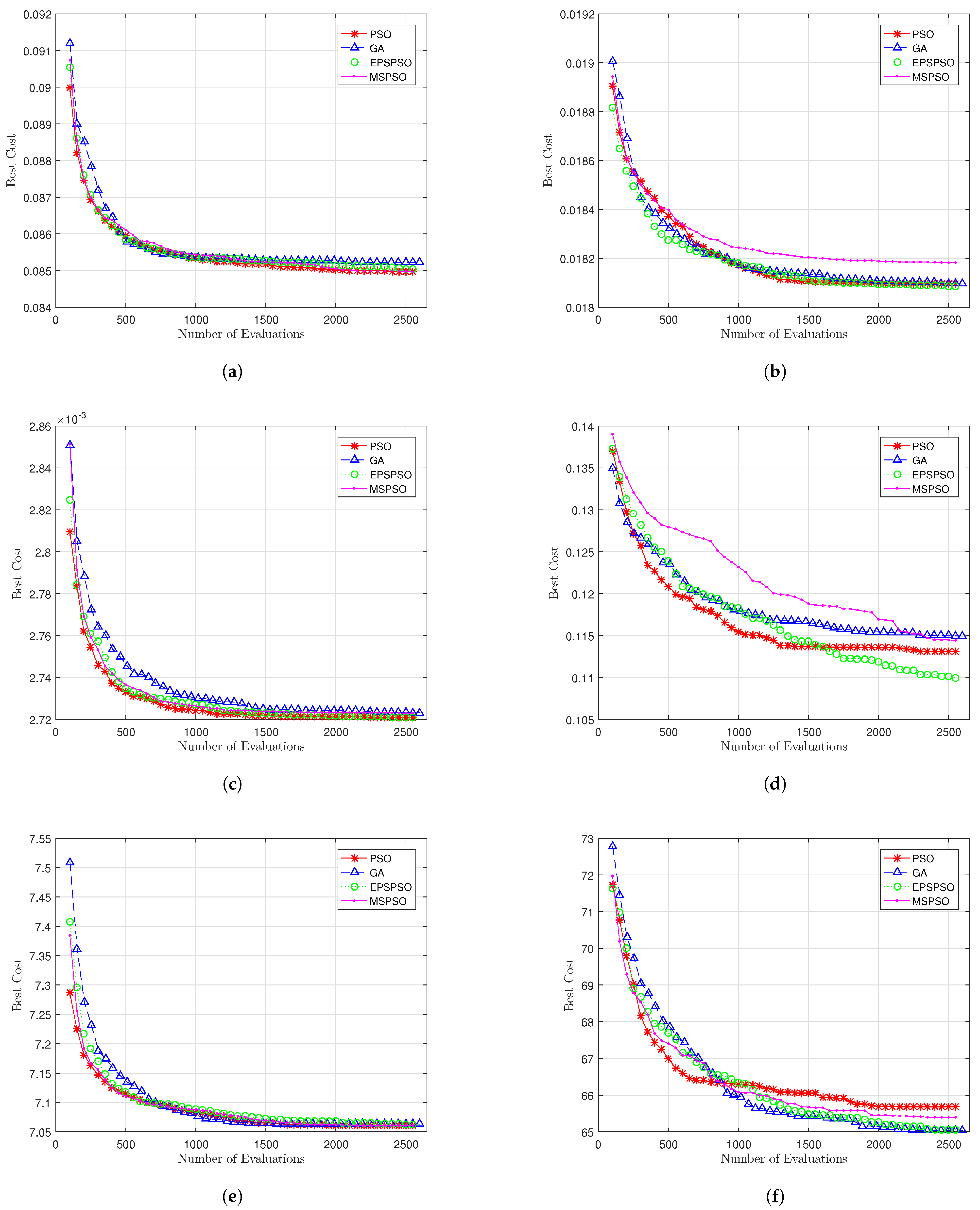
3.2. Parameters Optimization

In this section, we formalize a single-objective optimization problem:

$$\begin{array}{c}\hfill \min \left\{\mathrm{MSE}(\Gamma ,R_c)\right\},\\ \hfill \mathrm{subject}\mathrm{to}:\Gamma \in [0,5],R_c\in [0,1].\end{array}$$

(23)

The optimization has been performed using the described evolutionary optimization methods with the key parameters given in Table 44.

Table 44. Parameters of the considered optimization algorithms.

Algorithms	s	$\mathit{MaxIt}$	${\mathit{w}}_{\mathit{max}}$	${\mathit{w}}_{\mathit{min}}$	${\mathit{c}}_1={\mathit{c}}_2$	Additional
PSO	50	50	0.9	0.4	2
GA	50	50	/	/	/	$p_c=p_m=0.5$
EPSPSO	$25+25$	50	0.9	0.4	2	$t_g=5$
MSPSO	$25+25$	50	0.9	0.4	2	$nSwarm=2$

The number of particles in the swarm, s, the maximum number of iterations, $MaxIt$, and the corresponding parameters have been kept equal for all considered optimization algorithms to preserve the equal number of the MSE evaluations and to facilitate mutual comparison. That is, each swarm size in the EPS-PSO and MSPSO algorithms, which use multiple swarms, has been scaled accordingly to preserve s.

The computational results, including the average (Mean), the best (Best), the worst (Worst), the standard deviation (Std. Dev.), and the median (Median), obtained by the PSO-based and GA-based optimization algorithms applied to the parameters optimization problem for each considered noisy signal at the SNR of 7 dB, are given in Table 45. The convergence results for 50 independent runs are shown in Figure 8.

Table 45. The computational results obtained by the PSO-based and GA-based optimization algorithms after 50 iterations, averaged over 50 independent runs.

Signal	Statistic	PSO	GA	EPS-PSO	MSPSO
	Mean	0.0850	0.0852	0.0850	0.0850
	Best	0.0849	0.0849	0.0849	0.0849
Blocks	Worst	0.0854	0.0856	0.0854	0.0854
	Std. Dev.	$2.1332·{10}^{-4}$	$2.7481·{10}^{-4}$	$2.5420·{10}^{-4}$	$2.0457·{10}^{-4}$
	Median	0.0849	0.0854	0.0849	0.0849
	Mean	0.0181	0.0181	0.0181	0.0182
	Best	0.0181	0.0181	0.0181	0.0181
Bumps	Worst	0.0187	0.0184	0.0181	0.0189
	Std. Dev.	$8.8353·{10}^{-5}$	$5.3257·{10}^{-5}$	$8.3062·{10}^{-6}$	$2.4976·{10}^{-4}$
	Median	0.0181	0.0181	0.0181	0.0181
	Mean	0.0027	0.0027	0.0027	0.0027
	Best	0.0027	0.0027	0.0027	0.0027
Doppler	Worst	0.0027	0.0028	0.0027	0.0028
	Std. Dev.	$7.0885·{10}^{-7}$	$6.2548·{10}^{-6}$	$9.6431·{10}^{-7}$	$1.2469·{10}^{-5}$
	Median	0.0027	0.0027	0.0027	0.0027
	Mean	0.1131	0.1150	0.1100	0.1144
	Best	0.1070	0.1070	0.1070	0.1070
HeaviSine	Worst	0.1330	0.1330	0.1330	0.1333
	Std. Dev.	$1.10·{10}^{-2}$	$1.13·{10}^{-2}$	$8.10·{10}^{-3}$	$1.15·{10}^{-2}$
	Median	0.1070	0.1070	0.1070	0.1070
	Mean	7.0609	7.0632	7.0628	7.0609
	Best	7.0609	7.0609	7.0609	7.0609
Piece-Regular	Worst	7.0609	7.1043	7.0848	7.0609
	Std. Dev.	$3.5888·{10}^{-15}$	$8.3·{10}^{-3}$	$6.6·{10}^{-3}$	$3.5888·{10}^{-15}$
	Median	7.0609	7.0609	7.0609	7.0609
	Mean	65.6770	65.0317	65.0584	65.3961
	Best	64.1788	64.1788	64.1788	64.1788
Sing	Worst	68.8607	68.8607	68.8607	68.8607
	Std. Dev.	2.2062	1.7989	1.8182	2.0745
	Median	64.1788	64.1788	64.1788	64.1788

Figure 8. Convergence comparison between the considered optimization algorithms for signals: (a) Blocks. (b) Bumps. (c) Doppler. (d) HeaviSine. (e) Piece-Regular. (f) Sing.

All considered optimization algorithms have performed well for the Blocks signal. However, the PSO-based algorithms have a slight advantage over the GA with respect to the Worst, Std. Dev., and convergence, as shown in Figure 8a. All optimization algorithms have found the global optimum multiple times in 50 independent runs.

Similarly, high optimization performance is obtained for the Bumps signal, as well. The difference is with the GA, which performs equally well as the PSO-based algorithms in this case. The exception is the MSPSO algorithm, which provides the poorest performance with respect to the Mean, Worst, and Std. Dev. Additionally, Figure 8b clearly shows poorer convergence of the MSPSO algorithm. On the other hand, the EPS-PSO shows excellent performance, as it has converged to the global optimum in each independent run. Similar to the previous case, all optimization algorithms have found the global optimum at least once in 50 independent runs.

Excellent optimization performance is obtained for the Doppler signal. All considered optimization algorithms have found the global optimum numerous times in 50 independent runs, where the PSO and the EPS-PSO have converged to the global optimum in each optimization run.

The results obtained by the considered optimization algorithms differ the most for the HeaviSine signal example. Although all optimization algorithms have found the global optimum at least once in 50 independent runs, the obtained numerical results and graphical representation of the convergence suggest that the GA and the MSPSO have performed worse than the PSO and the EPS-PSO algorithms, with the EPS-PSO highlighted again as the best performing algorithm with respect to the obtained results statistics and convergence (Figure 8d).

Another high optimization performance is obtained for the Piece-Regular signal, similarly to the Doppler signal example. The only difference is that the MSPSO has replaced the EPS-PSO as the best performing algorithm along with the PSO, which has also found the global optimum in each independent run.

The optimization results for the final signal example, the Sing, highlight the MSPSO and, for the first time, the GA as the best performing algorithms with respect to the statistics and convergence, shown in Figure 8f. All considered optimizations algorithms perform with the equal Best and Worst solutions in 50 independent runs.

To sum up, all tested optimization algorithms perform well for our optimization problem, successfully finding the global optimum for all signal examples. The larger size of the single swarm in the PSO algorithm boosts the convergence for the initial number of evaluations. However, the EPS-PSO algorithm, with a greater ability to escape from the local optimum, stands out as the best performing optimization algorithm for our signal examples.

3.3. Experimental Results for Real-Life Signals

In order to test the proposed RBF-RICI filtering algorithm in real-life conditions, we have applied it to the noisy measured maritime signals (as an example of a practical application). The measurements were obtained from a buoy located in the Atlantic Ocean, approximately 210 nautical miles west-southwest of Slyne Head at the west coast of Ireland. The data is provided by Met Éireann, Ireland’s National Meteorological Service, as an open-access dataset publicly available at https://data.gov.ie/dataset/hourly-data-for-buoy-m6 (accessed on 17 April 2021). The dataset contains hourly measurements from 2006 to the present.

Figure 9a shows the noisy measurements of the sea temperature (°C), while Figure 9b,c show the sea temperature signal obtained after applying the RBF-RICI filtering algorithm and Savitzky–Golay filtering algorithm, respectively. The RBF-RICI algorithm’s parameters are set to $\Gamma =3.2$ and $R_c=0.9$. All real-life maritime signals considered in this analysis are filtered using the Savitzky–Golay filter with the second order polynomial and the window width set to $2\%$ of the signal length. This particular window width setting is chosen because the widths of that order of magnitude proved to be optimal during the analysis performed for several synthetic signals.

Figure 9. Sea temperature: (a) Noisy measured signal. (b) RBF-RICI filtered signal. (c) Savitzky–Golay filtered signal.

The measurements of the significant wave height (m) are shown in Figure 10a, while Figure 10b,c show the same data after application of the RBF-RICI and Savitzky–Golay filtering algorithm, respectively. In this case, the RBF-RICI parameters are set to $\Gamma =3$ and $R_c=0.1$.

Figure 10. Significant wave height: (a) Noisy measured signal. (b) RBF-RICI filtered signal. (c) Savitzky–Golay filtered signal.

Figure 11a shows the noisy measurements of the wave direction (°), whereas Figure 11b shows the wave direction signal obtained after applying the RBF-RICI filtering algorithm, whose parameters are tuned to the values $\Gamma =0.6$ and $R_c=1$. Figure 11c shows the signal obtained after application of the Savitzky–Golay filter.

Figure 11. Wave direction: (a) Noisy measured signal. (b) RBF-RICI filtered signal. (c) Savitzky–Golay filtered signal.

The measurements of the individual maximum wave height (m) are shown in Figure 12a, whereas Figure 12b shows the same data after application of the RBF-RICI filtering algorithm, whose parameters are set to the values $\Gamma =4.9$ and $R_c=0.95$. The Savitzky–Golay filtered signal is shown in Figure 12c.

Figure 12. Individual maximum wave height: (a) Noisy measured signal. (b) RBF-RICI filtered signal.(c) Savitzky–Golay filtered signal.

As shown in Figure 9, Figure 10, Figure 11 and Figure 12, the RBF-RICI filtering algorithm reduces the noise level in the real-life measurements and successfully reconstructs the main morphological features of the underlying signals, performing competitively to the conventionally applied Savitzky–Golay filtering algorithm. Therefore, the application of the RBF-RICI filtering enables better observation of the useful information and trends in the measurement data, and this way filtered signals may be used for further analysis and processing. Moreover, the RBF-RICI algorithm’s parameters $\Gamma$ and $R_c$ may be set to the values used as optimal for the simulated signals of similar morphologies. However, these parameters can be additionally adjusted in order to achieve the different levels of the filtered signal’s smoothness. The algorithm’s parameters obtained by this data-driven approach may be then successfully used for the filtering of the signals of the same type and similar characteristics.

4. Conclusions

In this paper, we proposed an adaptive RBF-RICI filtering algorithm, whose parameters are adjusted using the PSO-based procedure. The analysis of the RBF-RICI algorithm’s filtering performance was done using several synthetic noisy signals, showing that the algorithm is efficient in noise suppression and filtering error reduction. Moreover, comparing the proposed algorithm with similar filtering algorithms, we found that it shows better or competitive filtering performance in most considered test cases. Finally, we applied the proposed algorithm to the noisy measured maritime data, proving the possibility of its successful application in real-world practical applications. The possible other applications in the maritime sector include signals obtained by different ship measurement and detection sensors and systems, meteorological sea data, navigational data, etc. Moreover, the application of the proposed PSO-enhanced RBF-RICI filtering algorithm is not limited to the maritime transport sector only but may also be generalized for application in other fields dealing with nonstationary data.

References

- Broomhead, D.; King, G.P. Extracting qualitative dynamics from experimental data. Phys. D Nonlinear Phenom. 1986, 20, 217–236. [Google Scholar] [CrossRef]
- Smyth, A.; Wu, M. Multi-rate Kalman filtering for the data fusion of displacement and acceleration response measurements in dynamic system monitoring. Mech. Syst. Signal Process. 2007, 21, 706–723. [Google Scholar] [CrossRef]
- Knowles, I.; Renka, R.J. Methods for numerical differentiation of noisy data. Electron. J. Diff. Eqns. 2014, 21, 235–246. [Google Scholar]
- Layden, D.; Cappellaro, P. Spatial noise filtering through error correction for quantum sensing. Npj Quantum Inf. 2018, 4, 1–6. [Google Scholar] [CrossRef]
- García-Gil, D.; Luengo, J.; García, S.; Herrera, F. Enabling Smart Data: Noise filtering in Big Data classification. Inf. Sci. 2019, 479, 135–152. [Google Scholar] [CrossRef]
- Li, H.; Gedikli, E.D.; Lubbad, R. Exploring time-delay-based numerical differentiation using principal component analysis. Phys. A Stat. Mech. Its Appl. 2020, 556, 124839. [Google Scholar] [CrossRef]
- Zhao, Z.; Wang, S.; Wong, D.; Sun, C.; Yan, R.; Chen, X. Robust enhanced trend filtering with unknown noise. Signal Process. 2021, 180, 107889. [Google Scholar] [CrossRef]
- Ehlers, F.; Fox, W.; Maiwald, D.; Ulmke, M.; Wood, G. Advances in Signal Processing for Maritime Applications. EURASIP J. Adv. Signal Process. 2010. [Google Scholar] [CrossRef]
- Singer, A.C.; Nelson, J.K.; Kozat, S.S. Signal processing for underwater acoustic communications. IEEE Commun. Mag. 2009, 47, 90–96. [Google Scholar] [CrossRef]
- Sazontov, A.; Malekhanov, A. Matched field signal processing in underwater sound channels. Acoust. Phys. 2015, 61, 213–230. [Google Scholar] [CrossRef]
- Yuan, F.; Ke, X.; Cheng, E. Joint Representation and Recognition for Ship-Radiated Noise Based on Multimodal Deep Learning. J. Mar. Sci. Eng. 2019, 7, 380. [Google Scholar] [CrossRef]
- Tu, Q.; Yuan, F.; Yang, W.; Cheng, E. An Approach for Diver Passive Detection Based on the Established Model of Breathing Sound Emission. J. Mar. Sci. Eng. 2020, 8, 44. [Google Scholar] [CrossRef]
- Vicen-Bueno, R.; Carrasco-Álvarez, R.; Rosa-Zurera, M.; Nieto-Borge, J.C.; Jarabo-Amores, M.P. Artificial Neural Network-Based Clutter Reduction Systems for Ship Size Estimation in Maritime Radars. EURASIP J. Adv. Signal Process. 2010, 2010, 380473. [Google Scholar] [CrossRef]
- Ristic, B.; Rosenberg, L.; Kim, D.Y.; Guan, R. Bernoulli filter for tracking maritime targets using point measurements with amplitude. Signal Process. 2021, 181, 107919. [Google Scholar] [CrossRef]
- Schettini, R.; Corchs, S. Underwater Image Processing: State of the Art of Restoration and Image Enhancement Methods. EURASIP J. Adv. Signal Process. 2010, 2010, 746052. [Google Scholar] [CrossRef]
- Lu, H.; Li, Y.; Zhang, Y.; Chen, M.; Serikawa, S.; Kim, H. Underwater Optical Image Processing: A Comprehensive Review. Mob. Netw. Appl. 2017, 22, 1204–1211. [Google Scholar] [CrossRef]
- Huang, Y.; Li, W.; Yuan, F. Speckle Noise Reduction in Sonar Image Based on Adaptive Redundant Dictionary. J. Mar. Sci. Eng. 2020, 8, 761. [Google Scholar] [CrossRef]
- Ricci, R.; Francucci, M.; De Dominicis, L.; Ferri de Collibus, M.; Fornetti, G.; Guarneri, M.; Nuvoli, M.; Paglia, E.; Bartolini, L. Techniques for Effective Optical Noise Rejection in Amplitude-Modulated Laser Optical Radars for Underwater Three-Dimensional Imaging. EURASIP J. Adv. Signal Process. 2010, 2010, 958360. [Google Scholar] [CrossRef]
- Kim, K.S.; Lee, J.B.; Roh, M.I.; Han, K.M.; Lee, G.H. Prediction of Ocean Weather Based on Denoising AutoEncoder and Convolutional LSTM. J. Mar. Sci. Eng. 2020, 8, 805. [Google Scholar] [CrossRef]
- Yuan, J.; Guo, J.; Niu, Y.; Zhu, C.; Li, Z.; Liu, X. Denoising Effect of Jason-1 Altimeter Waveforms with Singular Spectrum Analysis: A Case Study of Modelling Mean Sea Surface Height over South China Sea. J. Mar. Sci. Eng. 2020, 8, 426. [Google Scholar] [CrossRef]
- Wei, J.; Xie, T.; Shi, M.; He, Q.; Wang, T.; Amirat, Y. Imbalance Fault Classification Based on VMD Denoising and S-LDA for Variable-Speed Marine Current Turbine. J. Mar. Sci. Eng. 2021, 9, 248. [Google Scholar] [CrossRef]
- Katkovnik, V.; Egiazarian, K.; Astola, J. Local Approximation Techniques in Signal and Image Processing; SPIE—The International Society for Optical Engineering: Bellingham, WA, USA, 2006. [Google Scholar] [CrossRef]
- Goldenshluger, A.; Nemirovski, A. On spatially adaptive estimation of nonparametric regression. Math. Methods Stat. 1997, 6, 135–170. [Google Scholar]
- Katkovnik, V. A new method for varying adaptive bandwidth selection. IEEE Trans. Signal Process. 1999, 47, 2567–2571. [Google Scholar] [CrossRef]
- Katkovnik, V.; Shmulevich, I. Kernel density estimation with adaptive varying window size. Pattern Recognit. Lett. 2002, 23, 1641–1648. [Google Scholar] [CrossRef]
- Lerga, J.; Vrankic, M.; Sucic, V. A Signal Denoising Method Based on the Improved ICI Rule. IEEE Signal Process. Lett. 2008, 15, 601–604. [Google Scholar] [CrossRef]
- Sucic, V.; Lerga, J.; Vrankic, M. Adaptive filter support selection for signal denoising based on the improved ICI rule. Digit. Signal Process. 2013, 23, 65–74. [Google Scholar] [CrossRef]
- Katkovnik, V. Multiresolution local polynomial regression: A new approach to pointwise spatial adaptation. Digit. Signal Process. 2005, 15, 73–116. [Google Scholar] [CrossRef][Green Version]
- Cai, Z. Weighted Nadaraya–Watson Regression Estimation. Stat. Probab. Lett. 2001, 51, 307–318. [Google Scholar] [CrossRef]
- Katkovnik, V.; Egiazarian, K.; Astola, J. Adaptive window size image de-noising based on intersection of confidence intervals (ICI) rule. J. Math. Imaging Vis. 2002, 16, 223–235. [Google Scholar] [CrossRef]
- Katkovnik, V.; Egiazarian, K.; Astola, J. Adaptive Varying Scale Methods in Image Processing; TTY Monistamo: Tampere, Finland, 2003; Volume 19. [Google Scholar]
- Lerga, J.; Sucic, V.; Sersic, D. Performance analysis of the LPA-RICI denoising method. In Proceedings of the 2009 6th International Symposium on Image and Signal Processing and Analysis, Salzburg, Austria, 16–18 September 2009; pp. 28–33. [Google Scholar] [CrossRef]
- Lopac, N.; Lerga, J.; Cuoco, E. Gravitational-Wave Burst Signals Denoising Based on the Adaptive Modification of the Intersection of Confidence Intervals Rule. Sensors 2020, 20, 6920. [Google Scholar] [CrossRef]
- Evangeline, S.I.; Rathika, P. Particle Swarm optimization Algorithm for Optimal Power Flow Incorporating Wind Farms. In Proceedings of the 2019 IEEE International Conference on Intelligent Techniques in Control, Optimization and Signal Processing (INCOS), Tamilnadu, India, 11–13 April 2019; pp. 1–4. [Google Scholar] [CrossRef]
- Fan, S.K.S.; Jen, C.H. An Enhanced Partial Search to Particle Swarm Optimization for Unconstrained Optimization. Mathematics 2019, 7, 357. [Google Scholar] [CrossRef]
- Garg, H. A hybrid PSO-GA algorithm for constrained optimization problems. Appl. Math. Comput. 2016, 274, 292–305. [Google Scholar] [CrossRef]
- Shen, Y.; Li, Y.; Kang, H.; Zhang, Y.; Sun, X.; Chen, Q.; Peng, J.; Wang, H. Research on Swarm Size of Multi-swarm Particle Swarm Optimization Algorithm. In Proceedings of the 2018 IEEE 4th International Conference on Computer and Communications (ICCC), Chengdu, China, 7–10 December 2018; pp. 2243–2247. [Google Scholar] [CrossRef]
- Donoho, D.L.; Johnstone, I.M. Adapting to Unknown Smoothness via Wavelet Shrinkage. J. Am. Stat. Assoc. 1995, 90, 1200–1224. [Google Scholar] [CrossRef]
- Schafer, R.W. What Is a Savitzky-Golay Filter? [Lecture Notes]. IEEE Signal Process. Mag. 2011, 28, 111–117. [Google Scholar] [CrossRef]
Publisher’s Note: MDPI stays neutral with regard to jurisdictional claims in published maps and institutional affiliations. |
© 2021 by the authors. Licensee MDPI, Basel, Switzerland. This article is an open access article distributed under the terms and conditions of the Creative Commons Attribution (CC BY) license (https://creativecommons.org/licenses/by/4.0/).