1. Introduction
The Yellow Sea (YS) is a semi-enclosed marginal sea in the northwestern Pacific connected to the Bohai Sea and the East China Sea on the north and south, respectively. The water depth of the YS is relatively shallow, with a mean value of approximately 44 m and a maximum value of 80 m in the central trough of the YS. The circulation in the YS is driven by tides, atmospheric forcing, oceanic flows and riverine discharges. Timko et al. [
1] included the YS as one of the coastal and shelf sea regions of the world where differences between global simulations with and without tides are mostly pronounced.
Pioneering studies on YS circulation have been conducted using two-dimensional barotropic tide models [
2,
3]. Attempts to model three-dimensional baroclinic circulation were first made by Lee [
4], but tidal forcing was not included in the application. Noting that strong tidal currents are omnipresent in coastal sea regions, Kang [
5] developed a three-dimensional diagnostic model considering M2 tidal forcing. The most important difference between the two baroclinic models was in the rotating direction of the mean circulation in the Yellow Sea. In detail, the model without tides produced anticyclonic circulation, while the model with tides produced cyclonic circulation. Since then, many studies using baroclinic models have been conducted in the YS, considering tidal forcing and/or wave effects [
6,
7,
8,
9,
10,
11].
The model configuration and input forcing used in the above baroclinic models are described below. Moon [
6] investigated how the coupling of waves and tides influences the modeling of oceanic circulation in the YS using the wave model WAVEWATCH II [
12] and the ocean model POM [
13]. The horizontal resolution was 1/6°. Tidal forcing was included together with monthly mean winds [
14], Levitus [
15] data and COADS (Comprehensive Ocean-Atmosphere Data Set). Xia et al. [
7] reported summer circulations using a POM-based wave-tide-circulation coupled model with a horizontal resolution of 1/6° and 16 vertical sigma layers. The model was driven by monthly climatological wind stress and net heat flux data [
16]. The initial temperature and salinity fields were prescribed using Levitus data [
15]. The MASNUM (Laboratory of Marine Science and Numerical Modeling, State Oceanic Administration) wave model [
17] was run with inputs of NCEP reanalyzed wind fields [
18]. Wave-induced vertical mixing computed from the MASNUM wave model was added to the vertical eddy viscosity and diffusivity produced by the turbulence closure scheme (TCS). Moon et al. [
8] carried out a range of calculations using a three-dimensional tide-ocean circulation coupled model called the RIAM Ocean Model developed by Lee [
4]. The model had a 1/6° horizontal resolution and 60 z levels. The vertical diffusivity was calculated using the turbulent kinetic energy equation introduced by Noh et al. [
19]. M2 tide and atmospheric forcing were used. Lü et al. [
9] studied the summertime vertical circulation in the YS using the model developed by Xia et al. [
7]. The horizontal resolution was improved to 1/12°, while the number of vertical layers was maintained at the same level. Particular attention was given to the upwelling near the tidal mixing front (TMF).
During the last decade, three important works were noted. Kwon et al. [
10] investigated the tidal stirring and wind mixing effects on the development of the summertime coastal boundary current along the eastern boundary of the YS using the ROMS model [
20]. The resolution was 1/12° on the horizontal plane and 30 s-coordinate levels in the vertical direction. Tidal forcing was included and the daily value of atmospheric forcing derived from the European Centre for Medium-Range Weather Forecast numerical prediction data was used. Initial temperature and salinity fields were prepared using 2007 results from the northwestern Pacific model integrated from 1993. Tidal stirring was found to play a major role in developing the boundary current in summer, while wind mixing made the current wider, increasing the northward transport. Kwak et al. [
11] carried out baroclinic simulations using the ROMS model considering turbidity and tidal mixing of the YS. The results of two well-known turbulence schemes (the Mellor–Yamada 2.5 closure scheme and the K-profile parameterization scheme) were compared, regarding the performance of reproducing temperature and salinity distributions in the YS. The Mellor–Yamada 2.5 scheme produced stronger vertical mixing and warmer bottom water than observations, while the K-profile parameterization scheme produced weaker vertical mixing than the Mellor–Yamada 2.5 scheme. Lee et al. [
21] compared the performance of three data assimilation techniques in simulating sea surface temperature in the YS. The ROMS model was used with a horizontal resolution of 1/10° and 30 vertical layers. The model was forced by tide and climatological heat fluxes. The modeling works described above are all process-oriented studies using climatological wind and heat flux data with relatively poor horizontal resolutions.
With the advancement of numerical modeling schemes and the accumulation of diverse observations, ocean forecast models have been developed over the last three to four decades and are now fully in operation. Typical examples include the U.S. Navy HYCOM and NEMO from France (for detailed information, see the summary given by Kim et al. [
22]). Park et al. [
23] reported the development of an operational forecast system for seas adjacent to the Korean Peninsula in the northwestern Pacific. YS circulation was predicted using the ROMS-based tide-wave-circulation model and the atmospheric WRF model. The model had a horizontal resolution of approximately 9 km and 30 vertical layers. Wang et al. [
24] used a POM-based circulation model coupled with surface waves, as did Xia et al. [
7], but without tides. The model had a horizontal resolution of 1/24° for the YS and ECS and 30 vertical layers. The model was linked to a larger northwestern Pacific model to derive open boundary information. The regional MM5 model supplied regional atmospheric forcing.
In this study, the COAWST system [
25] composed of the ocean model ROMS, the wave model SWAN and the atmospheric model WRF was applied to the YS. The long-term goal of this study was to establish an improved operational modeling system for the YS that was composed of a high-resolution, multiscale, baroclinic ocean model which is sufficiently validated and fully coupled in two ways to the operational atmospheric model. As a first step, a high-resolution coupled modeling system was established for the YS, focusing on the performance comparison of three TCSs (generic length scale, Mellor–Yamada 2.5 and K-profile parameterization abbreviated hereafter to GLS, MY2.5 and KPP, respectively) with regard to the simulated temperature and vertical temperature diffusion coefficients. Comparison studies of turbulence closure schemes were reported for the single process-dominated mixings, that is, either for tidal mixing [
26,
27,
28] or for wind mixing [
29] with relatively simplified topography. This study differs from previous comparison studies in that the performance of three TCSs was compared using a multiscale ocean model coupled with an atmospheric model in the YS with complex topography. From the outset, the focus of this comparison study was on identifying clues to judge the better performing TCS.
The contents of this paper are as follows.
Section 2 describes details of the Yellow Sea model and cross-sections where the results are compared.
Section 3 summarizes the model validations through error statistics, scatter plots, and cross-sectional distributions of temperature and vertical diffusion coefficients.
Section 4 contains conclusions.
2. Model
For the vertical mixing comparisons three turbulence closure schemes, GLS, KPP and MY2.5, were embedded in the ROMS model used. Two modeling domains were defined for the application of the COAWST system: one was a large domain for the atmospheric WRF model covering 114° E–132° E, 24.5° N–43.5° N, and the other was a small domain for the ocean circulation ROMS and SWAN wave model covering 116.5° E–127.5° E, 29.0° N–41.0° N (
Figure 1a). The atmosphere model WRF had a horizontal resolution of 1/10° (approximately 9 km) and 30 vertical levels, while the ocean models ROMS and SWAN had a horizontal resolution of 1/30° (approximately 3 km) and 30 vertical sigma layers. Therefore, the WRF model had 180 and 190 meshes in the longitudinal and latitudinal directions, respectively, while ROMS and SWAN had 330 and 360 meshes in the longitudinal and latitudinal directions, respectively.
Figure 1b shows the eastern side of the YS, where comparative results of turbulence closure schemes are presented. Lines 36° N (Line A) and 125° E (Line B) pass over sea regions where the so-called Yellow Sea Bottom Cold Water (YSBCW) is present in warm seasons. Line C passes over the shallow Yangtze bank. Line D was selected because it passes through the sea surface cold patch region off the Taean Penisula. At the late stage of this study, Line E was added along which Moon et al. [
8] and Lü et al. [
9] presented cross-sectional temperature distributions.
For the initial and boundary conditions of ROMS oceanic variables, HYCOM reanalysis data [
30] are used, while NOAA WW3 reanalysis data [
31] were used for the initial and boundary conditions of SWAN with the same resolution of ROMS. Tidal forcing information was obtained from TPX08 [
32]; eight harmonic constituents were used, such as M2, S2, N2, K2, K1, P1 and Q1. Tide levels were initially set to the mean sea surface height of the HYCOM data. The atmosphere model WRF used ECMWF ERA5 reanalysis data [
33] for initial and boundary conditions. Bathymetry was prepared using GEBCO data [
34]. WRF, ROMS and SWAN were two-way coupled. The coupling time between the ocean and atmosphere was set to 600 s. The wave model SWAN used a spectral directional resolution of 10° and 25 frequencies covering 0.04 Hz to 1 Hz. The computational time steps of WRF, ROMS and SWAN were 30, 20 and 120 s, respectively.
3. Results
Model runs were conducted for 16 days each season, including a five day spin-up period to suppress the possible influence of the initial fields. The simulation periods were 1–16 February, August and November 2018 and 9–24 May 2018. Comparative results from three turbulence closure schemes (TCSs) are described below.
3.1. Water-Level Validation
Comparison statistics of observed and computed water-level variations at full tidal station points were added as
supplementary materials. Note that since the simulation period was relatively short, each of the tidal harmonics cannot be separated; hence, we compared water-levels that contain tides and surges. It was not a strict comparison but may be sufficient for the purpose of the present study. Hence, water-levels containing tidal components and surges were compared. The observed water-level data came from KHOA (Korea Hydrographic and Oceanographic Agency, (
http://www.khoa.go.kr, accessed on 12 October 2021).
All three TCSs were found to reproduce overall water-level variations reasonably well, such as semidiurnal variation and spring-neap cycles (not shown here). RMSE values were large at tidal stations where tidal ranges were large (for example, Yeongheung-do where the spring tidal range reached approximately 800 cm), while they were relatively small at tidal stations where tidal ranges were small (for example, Seogwipo, approximately 180 cm). The maximum observed water-level range during the period was approximately 10 m. Surge heights in winter are usually larger than those in summer. Taking the average of 27 tidal stations in the model domain, the mean RMSEs of GLS, KPP and MY2.5 in February were 59.92 cm, 58.25 cm, and 56.54 cm, respectively, while in August they were 52.57 cm, 53.36 cm and 51.62 cm, respectively. Although the RMSE values varied spatially and seasonally, MY2.5 generally had the smallest mean RMSE, while GLS had the largest mean RMSE. The difference between the maximum and minimum RMSE was smaller than 5% of the mean RMSE value. Correlation coefficients (not shown here) exceeded 0.9.
From the statistics, it can be observed that the water-level differences produced by GLS and MY2.5 were very comparable, but the differences produced by KPP are larger than those produced by the GLS and MY2.5 results. The three vertical mixing coefficient values produced by the three TCSs are very different in time and space. The difference in vertical mixing produced different bottom frictional velocities, which in turn affected the bottom frictional dissipation, resulting in different tidal variations.
3.2. Wave Validation
Simulated wave heights were compared with measurements made by the KMA (Korea Meteorological Administration) using wave buoys. The simulated results were found to be in good agreement with the measurements. A comparison at a total of nine KMA wave measuring stations in the model domain (
https://www.kma.go.kr, accessed on 12 October 2021) provided RMSE values in February and August of 0.46 m and 0.31 m for GLS, 0.46 m and 0.33 m for KPP, and 0.46 m and 0.28 m for MY2.5, respectively. The correlation coefficients of GLS, KPP and MY2.5 in February were 0.85, 0.86 and 0.85, respectively, while in August, all three TCSs were 0.70. The maximum difference in wave heights between the TCSs’ results and observations during the period was approximately 40–60 cm. TCSs might affect current-wave interactions and air-sea interaction-related wind changes. However, as expected, the TCSs produced very marginal differences in wave heights. Comparison statistics of observed and computed significant wave heights are added as
supplementary materials.
3.3. Sea Surface Temperature Validation
Error statistics of sea surface temperature are computed, comparing simulated results with sea surface temperature values from KHOA and KMA buoy data. Full results of error statistics, which include BIAS (mean of (Predictions—Observations)), MAE (mean of (abs(Predictions—Observations))), and RMSE (root-mean-square of (Predictions—Observations)), are presented as
Supplementary Materials, Table S1.
Table 1 summarizes average values only.
It is evident from
Table 1 that the error parameters estimated using the KHOA buoy data are approximately 50% larger than those estimated using the KMA buoy data. The MAE and RMSE in August ware approximately 10 to 30% larger than those in February. The behaviors of BIAS values were quite different from other parameters. In February, the model overestimates the sea surface temperature, while in August, the model underestimates the sea surface temperature. The three TCSs produce similar results.
Some of the error parameters given in
Table 1 were compared with previous ROMS-based results [
21,
24]. Regarding the operational model accuracy for the YS, Park et al. [
24] presented RMSE and BIAS values for the sea surface temperature accuracy at four KMA buoy stations over the period of September 2011 and February 2012. RMSE results without data assimilation varied from 1.09 to 2.47 °C with a mean of 1.52 °C, while RMSE results with data assimilation varied from 0.69 to 2.36 °C with a mean of 1.19 °C. BIAS without data assimilation varied from −0.09 to 1.25 °C with a mean of 0.66 °C, while BIAS with data assimilation varied from −0.02 to 0.99 °C with a mean of 0.45 °C. Lee et al. [
21] performed a simulation study of temperature and presented monthly averaged RMSE values at four KMA buoy stations in August 2011 and February 2012, comparing measurements with model results computed both without and with data assimilation. In detail, the RMSE values without data assimilation were 1.64 °C (August) and 1.30 °C (February), while the RMSE values with data assimilation varied from 0.63 to 0.78 °C (August) and from 0.47 to 0.55 °C (February). It is worth noting that only the KMA buoy data were used in the above two studies. It is guessed that they were uncertain about the quality of the KHOA buoy data.
Although there were some limitations in direct comparisons of model results, the three TCSs produce results with smaller errors than those without assimilation but produce results with larger errors than those with assimilation. It is indicated that the model was reasonably well-constructed enough to identify which TCSs are better performing in temperature simulation.
3.4. Temperature and Salinity Scatter Plots
Figure 2 shows the seasonal T-S diagrams and the T-S surface-bottom difference diagrams in sea regions west of the Korean Peninsula covering 124° E–127° E and 32° N–38° N (Region 1 in
Figure 1b) reproduced using the three TCSs. In addition, HYCOM reanalysis results are included for comparison purposes. The sea region for the comparison was chosen because observations by the NIFS (National Institute of Fisheries Sciences), Korea, (
http://www.nifs.go.kr, accessed on 12 October 2021) were available. Examination of the two diagrams may be the simplest way to compare the overall performance between the three TCSs. The observations were instantaneous values, while the model results were daily averages. The contour lines of the T-S diagrams shown in
Figure 2 represent the density of sea water computed using the UNESCO algorithm [
35].
It is evident from
Figure 2 that all TCSs similarly reproduced the water mass distribution in winter with accuracy comparable to NIFS observations, while they reproduced considerably different distribution patterns for other seasons with accuracy less comparable to NIFS observations. The sea surface and sea bottom T-S differences have shown a distribution more or less similar to T-S diagrams but with larger deviation from NIFS observations than temperature. It can be inferred that these features may be associated with the degree of vertical stratification in each season. The low saline water reflects riverine influence from the Yangtze River.
To examine in more detail the summertime performance of the three TCSs and the HYCOM reanalysis results in Region 1, each of their results is separately represented in
Figure 3. The cross symbols are NIFS observations again, but colors represent scatter density computed using Gaussian kernel estimation. Note that on these days, the scatter density was of popular use to better present high concentration areas where dots heavily overlap. The HYCOM reanalysis results and the three TCSs reproduced T-S diagrams that were consistent with each other, producing results with slightly higher salinity than NIFS observations. For the case of the T-S surface-bottom difference, the computed distributions revealed considerable differences when compared with NIFS observations. The results of the three TCSs and the HYCOM reanalysis revealed some differences, mainly due to the discrepancies in surface-bottom salinity differences. The difference between the TCSs and the HYCOM reanalysis results reflects differences in numerical features other than TCSs. There could be many reasons why the HYCOM reanalysis results were significantly different from the three TCS models, but the most important point is that HYCOM does not consider tidal input, which induces the primary circulation and controls the water mass distribution in the YS. In the absence of tidal forcing, the bottom friction along the coastal water can be reduced more than ten times, and the vertical mixing was similarly reduced. Unrealistic stratification may also occur in shallow coastal waters. Indeed, various erroneous results can be produced in the YS. Such deficiencies can be recovered in part through the application of data assimilation. It is, however, believed that assimilation without proper dynamics obviously has limitations.
Figure 4 shows the T-S diagrams in sea regions covering 124° E–127° E and 32° N–34° N (Region 2 in
Figure 1b), which were chosen because the T-S surface and bottom difference is comparatively large due to the presence of prevailing oceanic currents.
An examination of the diagrams shows the presence of considerably large discrepancies of the T-S surface-bottom difference between the TCSs, while T-S diagrams are more or less close to each other. It is noted that KPP provides larger values of scatter in salinity than GLS and MY2.5.
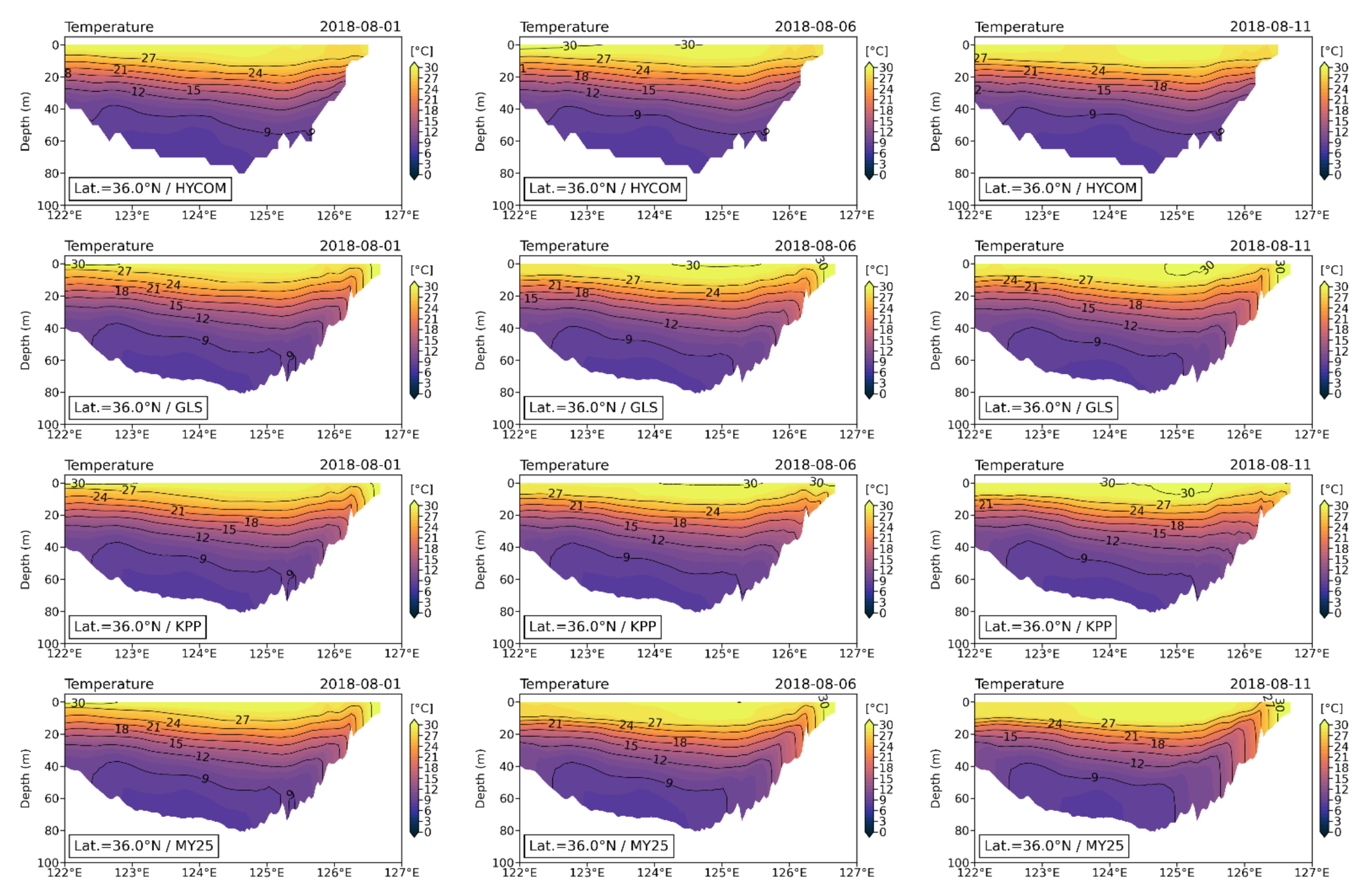
3.5. Temperature and Salinity Distribution along 36° N (Line A) and 125° E (Line B)
Both Lines 36° N and 125° E pass through the Yellow Sea central trough, where Yellow Sea Bottom Cold Water is known to exist from spring to autumn. This line has been chosen in many past studies [
7,
10,
36]. This line was primarily chosen to examine how much the use of HYCOM reanalysis results as initial conditions influences the subsequent calculation of the temperature field. Therefore, cross-sectional temperature fields along 36° N on 1, 6 and 16 August 2018 are presented in
Figure 5. At a very early stage, the results of all three TCSs were not much different from the HYCOM reanalysis temperature fields, probably because the influence of the initial field remains high. However, as time passed, the initial field impact disappeared, and the temperature fields of the three TCSs tend to deviate from the HYCOM reanalysis results and each other due to the difference in vertical mixing and air-sea interaction. The MY2.5 results appear to be more comparable with HYCOM results in comparison to the other two TCSs in that there was a thicker surface mixed layer than in the other two TCSs.
Line 125° E extending from 35° N to 34° N was considered by Lie [
37] to investigate the observed structures of temperature and salinity fields in the central YS (Line A considered here is further extended to 33° N). A considerable amount of work has been devoted to Yellow Sea Bottom Cold Water (YSBCW), which is often called the Yellow Sea Cold Water Mass (YSCWM), Yellow Sea Cold Water (YSCW) or Hwanghae Cold Water (HHCW). Cooling of the surface water during the winter monsoon leads to the formation of bottom cold water. The YSBCW occupies the bottom layer of the central Yellow Sea during spring to fall, in which a strong thermocline separates cold and salty bottom water from warm and fresh surface water. In the past, the YSBCW had long been accepted to have a temperature below 10 °C and a salinity of 32.0–32.5 psu. Based on the CTD observations conducted in August 1983, Lie [
37] defined the YSBCW water mass as having a salinity of 32.0–33.0 psu and a temperature below 10 °C. Zhu et al. [
36] used 8 °C as a temperature criterion in recent studies on the YSBCW. According to observations by Lie [
37] (not shown), the 10 °C isotherm was formed approximately 40 m below the sea surface in the sea region between 34.15° N and 35.05° N, while the 32.5 psu isohaline was located at a 20–25 m depth.
Figure 6 shows cross-sectional distributions of temperature and salinity along 125° E on 11 August 2018, computed using the three TCSs. MY2.5 produced a 10 °C isotherm depth closer to the observation by Lie [
37] than GLS and KPP. However, unlike the temperature distributions, the three TCSs poorly reproduced the salinity distributions, giving 0.5–1.5 psu higher values than the observations near the sea surface south of Line 125° E, which may be due to the difference in the influence of Changjiang river discharge. Therefore, it was appropriate to mention that the comparison results shown in this subsection are not sufficient to determine the better performing TCS.
Next, the cross-sectional thermal diffusion coefficient fields along 125° E computed using the three TCSs were examined. The results on 6, 11 and 16 August 2018, are shown in
Figure 7. It is evident that the thermal diffusion coefficients computed from the three TCSs are significantly different from each other. All TCSs basically produced three-layered structures, but as time passed, the thickness and thermal diffusion coefficient value of each layer markedly changed. MY2.5 produced the largest values of surface and bottom layer thickness, as well as the highest value of thermal diffusion coefficients at the surface and bottom layers, while KPP produced the lowest value of thermal diffusion coefficients and thickness at the bottom layer. In the case of the surface layer, the GLS and KPP results were comparable to each other. Note that in the middle layer, GLS produced the highest value of thermal diffusion coefficients, while MY2.5 produced the lowest. Subsequently, MY2.5 produced a very thin middle layer with diffusion coefficient values lower than 0.1 cm
2/s, as seen in the results on 16 August 2018.
It may be worthwhile to elaborate on the eddy diffusivity profiles in past studies. On the basis of temperature observation records in the central YS (36° N, 124° E), Dai et al. [
38] estimated the mean diffusion coefficients in the upper and midlayers in August as 1.2 cm
2/s and 0.14 cm
2/s, respectively. Kwak et al. [
11] presented the vertical temperature diffusion coefficient profiles at two points along 36° N computed without tides using KPP and MY2.5 embedded in ROMS. MY2.5 produced six times larger values of the vertical temperature diffusion coefficient than KPP, giving a maximum of 1800~2000 cm
2/s. Both TCSs produced minimum values close to the background level at the sea surface and sea bottom.
3.6. Temperature and Salinity Distribution along 32° N (Line C)
The 32° N line was chosen because some interesting differences in temperature distribution between the HYCOM reanalysis results and the three TCSs were noted in the preliminary numerical experiments.
Figure 8 shows the time evolution of the cross-sectional distributions of temperature along 32° N on 1, 6, 11 and 16 August 2018, computed using the three TCSs. Note that GLS and MY2.5 produced isotherm patterns very different from KPP, especially in the slope region between 125° E and 126° E.
Close examination reveals that on 1 August, all three TCSs showed a tendency such that the cold bottom water gradually moved toward the sea surface. That is, upwelling features occurred similar to the simulation by Lü et al. [
9]. As time passed, GLS and MY2.5 resulted in continuing the uprising of low temperatures to the surface, consequently forming cold patches on the sea surface. GLS and MY2.5 produced similar isotherm patterns, while KPP maintained the surface mixed layer. It was also interesting to note that in the relatively flat region with a depth of 40 m, vertically well-mixed structures of temperature were shown for the GLS and MY2.5 cases, while a complicated two-layered structure was shown for the case of KPP. We can see that the occurrence of upwelling depends on whether the tidal mixing front with a sharp horizontal gradient of temperature was formed.
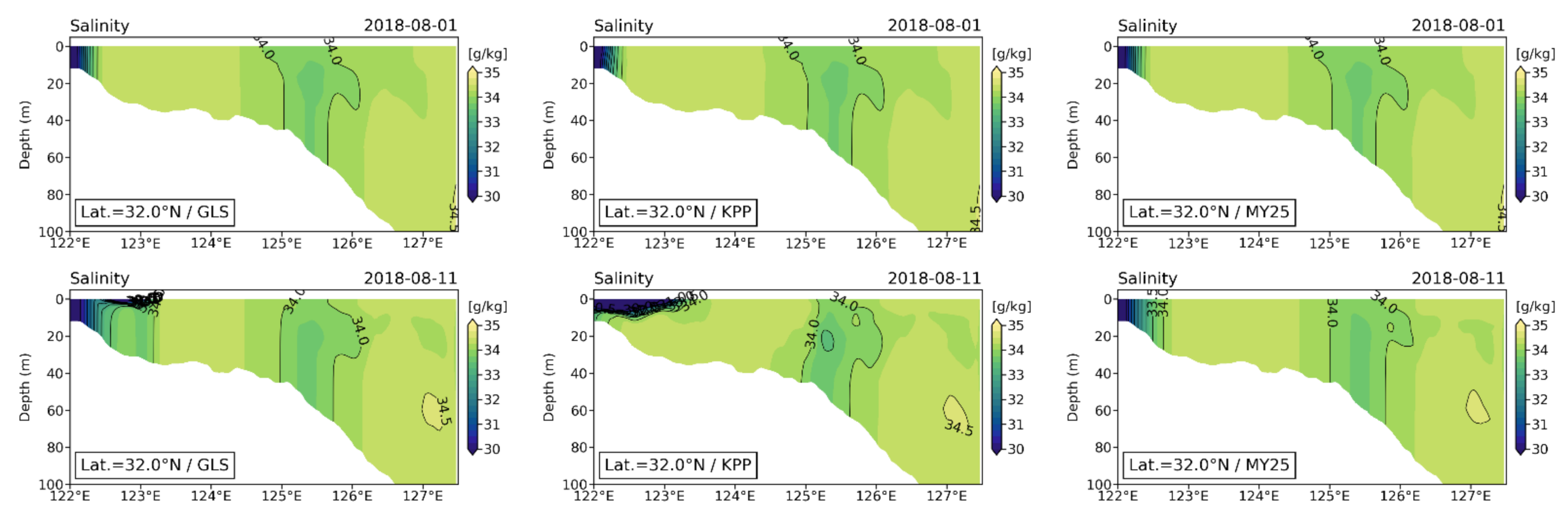
Figure 9 shows the cross-sectional distributions of salinity along 32° N on 1 and 11 August 2018, computed using the three TCSs. The patterns shown in the temperature fields did not appear, but slightly low salinity water remained throughout the computation period in a vertically well-mixed form. In the left corner of Line C near 122° E, the intrusion of freshwaters originating from the Changjiang River of mainland China can be seen. There was a possibility that part of the Changjiang River water transported to the north at latitudes higher than 32° N might have moved southward along with tidal residual flows.
It may be worth commenting on the study by Jang et al. [
39] in which the vertical distribution of mean temperature and salinity distributions (averaged over the 2003 to 2009 periods) were presented on the western slope of the YS central trough, in detail, along the transect 33° N between 124° E and 128° E. It was noted that the bottom of the surface mixed layer and strong thermocline was located at depths of approximately 10 m and 30 m, respectively. Unlike Lü et al. [
9], no evidence of upwelling was found. In the case of salinity, there were some hints that the influence of Changjiang diluted water expanding from the west existed near the surface of 124° E.
Figure 10 shows time variations of cross-sectional distributions of temperature diffusion coefficients along 32° N on 1, 6, 11 and 16 August 2018, computed using the three TCSs. The overall features of the temperature diffusion coefficient distributions are similar to those shown for 125° E. Examination of the diffusion coefficient field indicates that the occurrence of upwelling shown in
Figure 8 might be associated with the intensity of thermal diffusivity fronts. Strong thermal diffusion coefficient fronts formed for GLS and MY2.5, while weak fronts formed for KPP. Note that GLS and MY2.5 produced spatially homogeneous structures of thermal diffusion coefficients with values significantly larger than KPP.
3.7. T and S Variations along the Tidal Channel off the Taean Peninsula (Line D)
Choi et al. [
40] reported that the coldest surface was always observed over the deep channel with depths greater than 50 m off the Taean Peninsula, irrespective of the observation period. According to Lü et al. [
9], there are approximately five well-known sea regions in the YS where intense surface cold patches exist, and field observations and satellite images reveal this feature. The tidal channel off the Taean Peninsula is one of them. Line D passes through the region approximately parallel to the deep tidal channel.
Figure 11 shows the cross-sectional distributions of temperature along Line D on 1, 6, 11 and 16 August 2018, computed using the three TCSs. The temperature fields on 1 August 2018, were strongly influenced by the initial temperature fields. A small difference between the computed temperature fields supports this observation. As time passed, different features became pronounced. GLS and MY2.5 resulted in the formation of a surface cold patch region between approximately 125.8° E and 126.2° E, forming a tidal mixing front, while KPP scarcely provided any hints of forming a tidal mixing front. Generally, localized surface cooling of approximately 2–4 °C occurred in the GLS and MY2.5 results, while localized surface cooling of less than 2 °C occurred in the case of KPP.
Figure 12 shows cross-sectional distributions of salinity along Line D on 1 and 11 August 2018, computed using the three TCSs. From close examination of the results, we found that KPP produced slightly stronger stratification than GLS and MY2.5. At the shallow north end, the salinity values gradually decreased. This decrease might be due to the Han River discharge.
Figure 13 shows cross-sectional distributions of salinity along Line D on 1, 6 and 11 August 2018, computed using the three TCSs. The overall patterns and magnitude of the vertical mixing coefficients are similar to those shown along 32° N. However, the spatial gradient of vertical mixing coefficient contours computed using GLS and MY2.5 appears to be less steep than those computed along the slope of 32° N. Furthermore, complex bottom topography exists in this region. We therefore infer that the formation mechanism of localized surface cold patches in this region might be different from the case along 32° N.
3.8. Temperature Distribution along 34° N (Line E)
Finally, the cross-sectional distributions of temperature along 34° N (Line E) were compared. The presence of a cold patch near the western end of Line E (122° E–122.3° E with a depth of approximately 20 m) is well known from satellite data and in-situ measurements (see Lü et al. [
9]).
Figure 14 shows that GLS and MY2.5 clearly reproduced the cold patch, while KPP hardly reproduced its presence.
A mechanism of cold patch formation in the TMF near the Chinese shallow coastal zone of approximately 20 m depth (122° E–122.3° E) was presented by Lü et al. [
9] using the same POM as Xia et al. [
7]. Moon et al. [
8] also reproduced the cold patch through the comparison of the computed results with the observed temperature distribution shown in the Yellow Sea Atlas (Lee et al. [
41]). Again, from the cross-sectional distributions of the vertical eddy diffusion coefficients, it can be seen that GLS and MY2.5 obviously produced vertical mixing stronger than KPP at both the surface and bottom layers.
4. Conclusions
In this study, the performance of three TCSs embedded in ROMS as part of the COAWST system was compared with particular emphasis on the reproduction of temperature distributions in the Yellow Sea. For that, a three-dimensional baroclinic model with a fine resolution (horizontal resolution of 1/30° and 30 vertical sigma layers) was developed and then applied to the YS, where multiple oceanic processes (tide, wave and oceanic circulation) and air-sea interactions control the water mass structure and circulation. For the initial conditions, HYCOM reanalysis data were used. Model validations were performed comparing water-level, wave and sea surface data supplied by KHOA and KMA. The three TCSs produced comparable validation results, although some discrepancies and inconsistent patterns were found in the sea surface temperature results. A comparison with previous model results showed that the model constructed in this study produced sea surface temperature distributions with accuracy better than that without data assimilation, but worse than that with data assimilation. It could be said that the model can be used with confidence to identify which TCSs were better performing in temperature simulation in the YS.
Two regions (Region 1 and Region 2) and a total of five lines were considered for the comparison, mainly temperature distributions. Lines A and B pass through the central YS, where the YSBCW exists from spring to autumn. The performance results of the three TCSs were qualitatively compared in the two box regions (Region 1 and Region 2) through T-S diagrams and surface and bottom T-S difference diagrams. In an overall sense, the performance results of the three TCSs were found to be quite comparable, although there were obvious discrepancies between the observed and computed values.
A comparison of the overall features of cross-sectional temperature distributions along the five lines revealed that GLS and MY2.5 obviously produced vertical mixing stronger than KPP at both the surface and bottom layers. Kwak et al. [
11] obtained similar results from the comparison between KPP and MY2.5. However, such results were sufficient to determine the better performing TCS in terms of the difference in large-scale features of temperature distribution.
The identification of the better performing TCS in this study was limited possibly based on the simulation capability of cold patches in the TMF. GLS and MY2.5 clearly reproduced the cold patch located near the western end of Line E (122° E–122.3° E with a depth of approximately 20 m), while KPP hardly reproduced its presence. Similar results were obtained along Line D but with a less pronounced TMF. Note that the presence of a cold patch in Line E and its formation mechanism associated with upwelling in the TMF region were confirmed in previous studies [
8,
9]. The results from Lines D and E indicate that the performance of GLS and MY2.5 is better than that of KPP in the YS with multiscale processes. Surprisingly, GLS and MY2.5 produced cold patches on the western slope of the Yellow Sea trough (approximately 40 m depth), the presence of which had never been reported in observations and model results. Of course, evidence of cold patches was absent in the results from KPP. To deduce more definite conclusions on the performance of the three TCSs more observational data are required. In detail, measurements at two sites were recommended for future studies: one was the measurement of temperature and salinity profiles along 32° N (Line C in
Figure 1b), especially near 125° E–126° E, and the other was the measurement of temperature and salinity profiles along the tidal channel off the Taean Peninsula (Line D in
Figure 1b). With the acquisition of good-quality data, rigorous comparison experiments are required to achieve the long-term goal of securing a reliable operational system.
There may be two main issues related to the improvement of operational modeling in the YS. One is how to improve the initial and boundary conditions of ocean models, and the other is how to improve the interaction between the atmospheric and ocean models. To date, assimilation of satellite-based sea surface temperature information has been used to obtain better initial and boundary conditions. Assimilation of sea surface height data, which play an important role in open ocean modeling, has not been used in the YS, probably because of technical difficulties due to high tide. Fortunately, such difficulty might soon be overcome because HYCOM-related researchers are devoted to developing a technique for incorporating tidal variations. Subsequently, expanding the data assimilation is one of the research themes in the long-term goal of the study. The other is in fact a global issue closely related to vertical mixing parameterizations at the sea surface and within the water column. More attention has recently been paid to the momentum and heat exchange between the air and sea as the YS region experiences the passage of strong typhoons in summer and autumn. To improve the air-sea interaction process, parameterizations of sea spray effects and wave-induced vertical mixings should be incorporated. Additionally, a suspended sediment model should be developed and validated because the high turbidity of the YS can control heat penetration through the water column. As found in this study, the fine structure of the interaction between the near-surface and bottom boundary layers needs to be clarified with regard to TCSs.
The possible use of data assimilation, the selection of the best performing TCS with possible modification, incorporating a better air-sea interaction formula and extension of the model domain should be considered in future studies.


