Hydro- and Morphodynamic Impacts of Sea Level Rise: The Minho Estuary Case Study

Abstract

The understanding and anticipating of climate change impacts is one of the greatest challenges for humanity. It is already known that, until the end of the 21st century, the mean sea level (MSL) will rise at a global scale, but its effects at the local scale need to be further analyzed. In this context, a numerical modelling tool and a methodological approach for the river Minho estuary (NW of the Iberian Peninsula) are presented, to predict possible consequences of local MSL rise, considering the greenhouse emission scenarios RCP 4.5 and RCP 8.5. Hydrodynamic and morphodynamic impacts were analyzed considering several driving factors, such as tides, sea level rise, storm surge, wave set-up, and different river flood peak discharges, taking into account their probabilities of occurrence. The model was calibrated using in-situ data and a data assimilation tool, the OpenDA, which automates this process, allowing to reach reliable results in a considerably short time when compared with traditional techniques. The results forecast that the predicted MSL rise will reduce the flow velocity magnitude and the sediment transport into the coastal platform but will aggravate the inundation risks along the estuarine banks. In the worst scenario (RCP 8.5) the water level near the river mouth of the estuary is expected to rise 0.20 m for 50 years return period ocean water rising, and 0.60 m for 100 years return period. It was also possible to identify that floods are the most important driver for the sediment transport along the estuary, while the tide effect in the morphodynamics is restricted to the downstream estuarine region. This work demonstrated the importance of the numerical modelling tools to better understand the effects of climate change at local scales through the representation of the estuarine hydrodynamic pattern evolution for future climate scenarios.

1. Introduction

In the last decades, climate change effects on the water cycle have been observed on a global scale. After the second half of the 21st century, an increase in the frequency of extreme events, such as storms, floods, and droughts, is likely, moving from a return period (RP) longer than 100 years to annual occurrences [1]. Besides, climate change will result in higher atmospheric and oceanic mean temperatures, promoting the thermal expansion of water bodies that, jointly with land-ice melting, will result in higher mean sea level (MSL) and extreme sea levels (ESL) [1,2].

A rapid growth in population and economic assets in coastal zones and floodplains has been observed and it is expected to continue during the next years [3]. The coastward migration of the population can be explained by the great economic and environmental values of these regions, which can be translated into high population concentration, increased urbanization, and intensification of coastal agricultural and industrial activities [4,5]. These facts augment the vulnerability of coastal regions to climate change effects due to the sea level rise combined with increased risks of storms, intense rainfall, and flash floods [6]. However, it is important to take into account that the sea level change is far from being uniform along the temporal and spatial scales, due to the influence of oceanic currents, land ice mass loss, land water storage variation, ocean thermal expansion, and water density changes [7,8,9]. Therefore, it is important to perform local studies to accurately represent the effects of climate change for small regions, particularly morpho-hydrodynamic studies.

Understanding the erosion and accretion processes in coastal areas, and accurately forecasting their evolution, is essential in order to prioritize mitigation measures and manage planning decisions [10]. A commonly accepted methodology to predict and evaluate future scenarios is the implementation of numerical models, which are essential tools to forecast the effects of floods and extreme events in estuarine regions [11].

This paper presents a numerical model, implemented with the Delft3D software (Deltares, Delft, The Netherlands) [12], developed to forecast the possible impacts of climate change on the hydrodynamic and morphodynamic patterns in the Minho estuary. The model was calibrated using the data assimilator OpenDA [13] to achieve the most adequate calibration parametric values, while reducing the time needed for this task. Although the developed work is focused on impacts of sea level rising due to climate change there are other aspects that can also influence the relative sea level position in coastal areas. Leorri et al. [14] analyzed sea level evolution considering tectonic movements. Rovira et al. [15] studied sediment imbalances, identifying the Minho estuary as one of the European estuaries that is affected by sediment accumulation, which can also affect water levels within the estuary.

2. Study Area and Methods

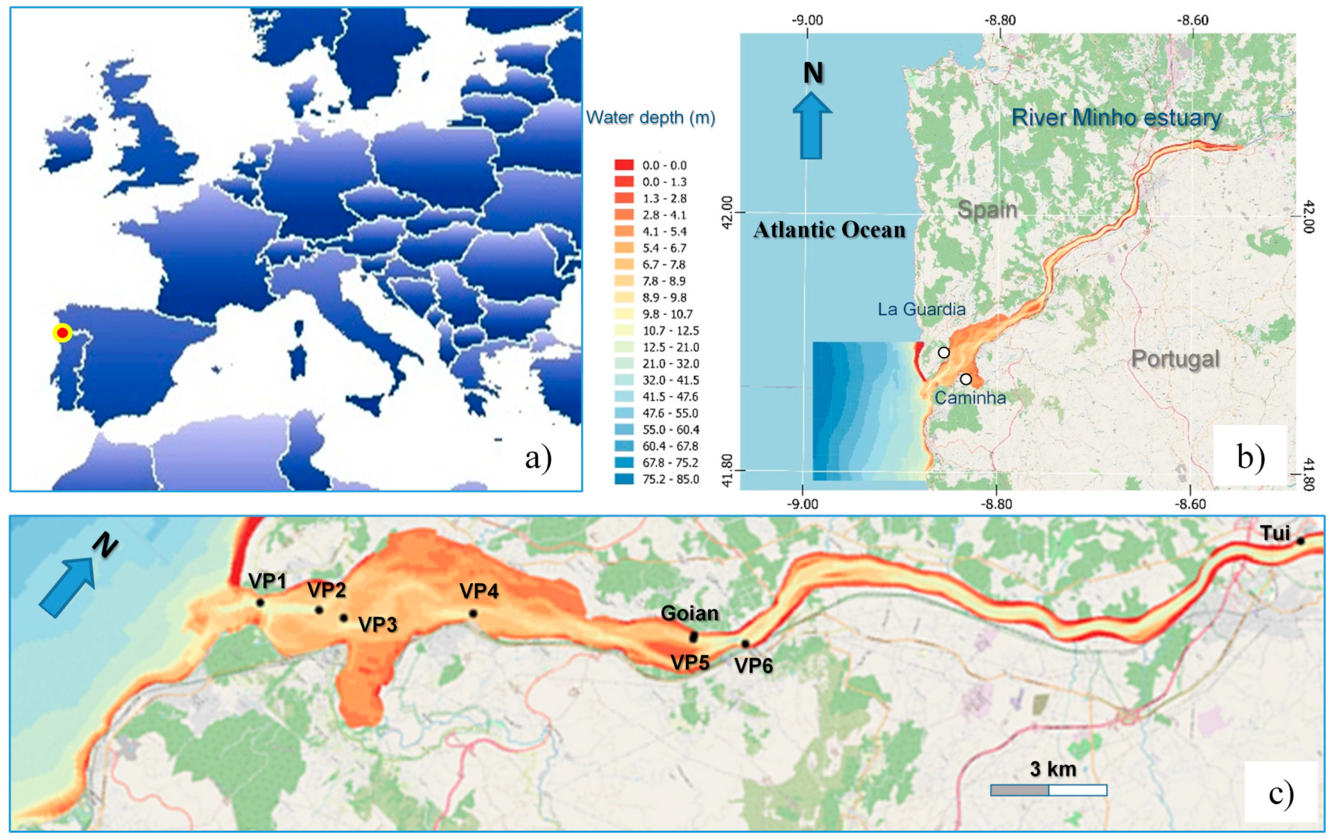
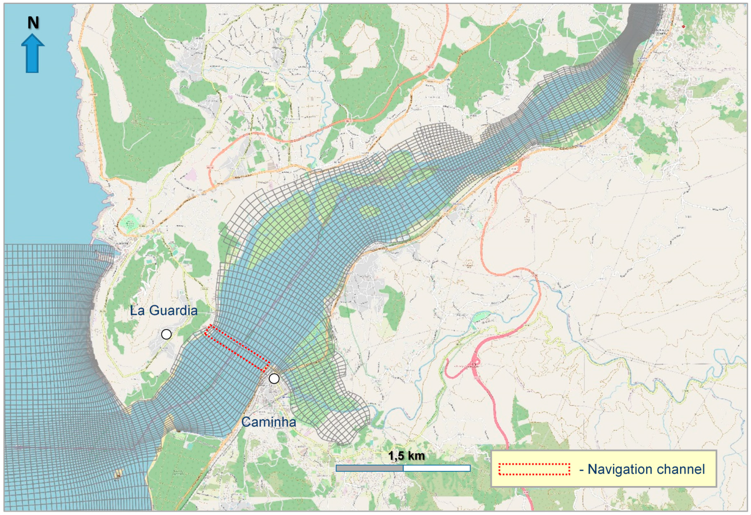
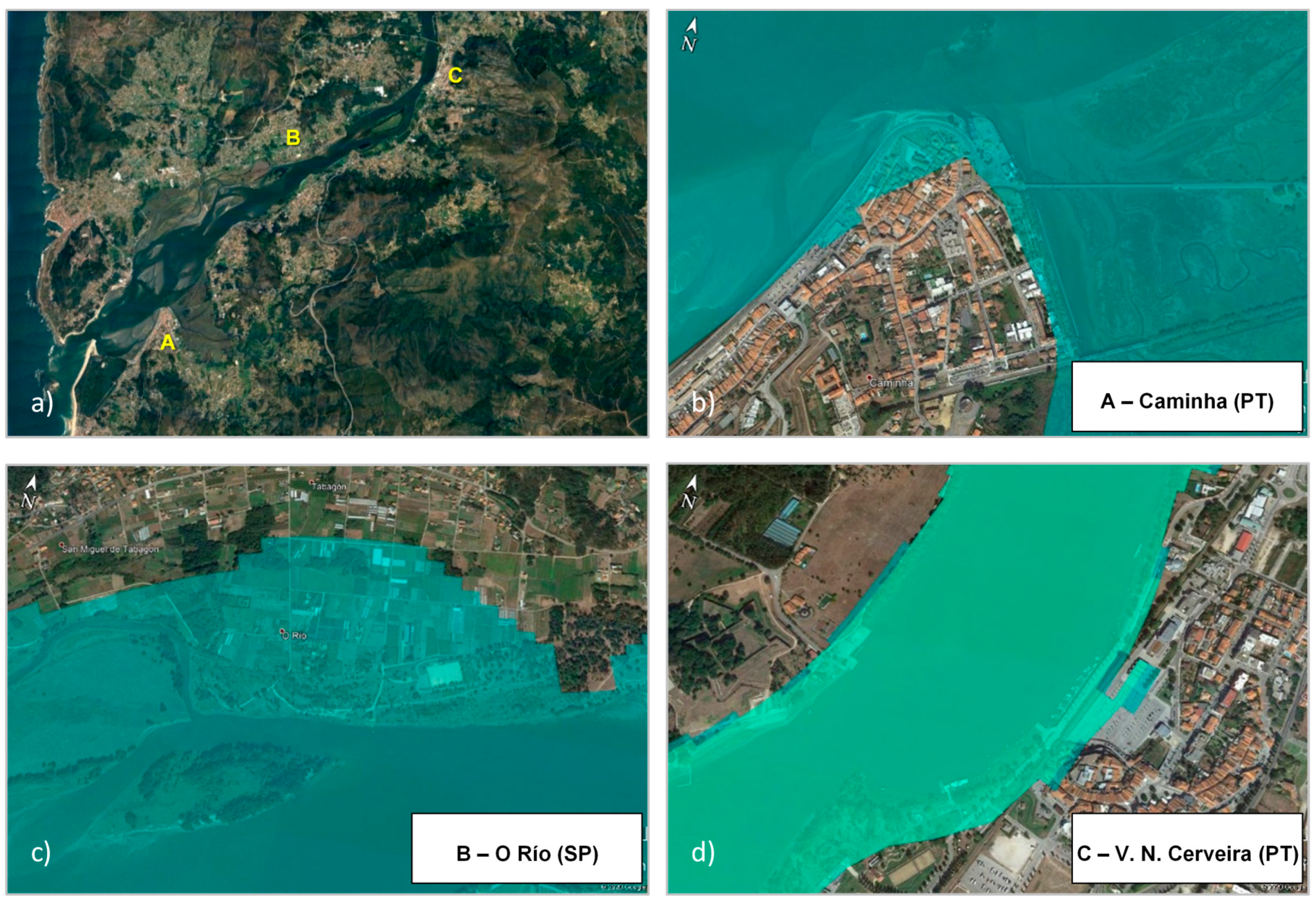
2.1. Study Area

The Minho is an international river that rises at the Serra de Meira, in Spain, and reaches the Atlantic Ocean between Caminha (Portugal) and La Guardia (Spain) after 340 km, constituting a natural border between the northern Portuguese and Galician regions in its last 70 km (Figure 1). This river plays an important role in hydropower production, tourism, and wine production, and its estuary presents a large diversity of habitats due to its good ecological quality, being a reference in ecotoxicological studies and an example for the implementation of water directives in other rivers [16,17]. In the estuarine area, there is a ferryboat that connects the riverside cities of Caminha and La Guardia, whose operation is conditioned by water level oscillations (dependent on tides, sea level, and river flow) and by the morphodynamics of the estuary (Figure 2).

The average annual river flow is 300 m³/s, oscillating between 100 m³/s in the dry season (summer) and 500 m³/s in the wet season (winter). River flow depends on the precipitation patterns over the hydrographic basin and on the Frieira dam discharges, located 80 km upstream of the estuary mouth [18,19]. The lower estuary presents an accentuated enlargement which results in a decrease of the velocity of the current, creating favorable conditions for sediment deposition. Siltation is one of the main problems of this estuarine region [17]. The annual average temperature of the water is 14 °C [20]. Next to being considered a low-impacted estuary in terms of human intervention, freshwater discharges from the river Minho have an important effect on the nearby ocean ecosystems, promoting phytoplankton growth and biodiversity in the coastal area through its river plume intrusion [21]. This is especially relevant for the local fishery and for the river to be considered as a natural heritage resource, which brings a relatively intense touristic activity to the region, also related with a highly valued wine production activity.

Consequences of sea level rise (SLR), like inundations and possible saltwater intrusion can compromise all these activities, justifying the necessity and importance of anticipating the effects of climate change on the hydro-morphodynamic patterns within this estuary. It is essential to predict the effects of hazardous and extreme events, to pinpoint estuarine fragilities and vulnerabilities, and to provide valuable information to managers and authorities responsible for the safety of populations, properties, and economical activities, to promote effective and integrated coastal management.

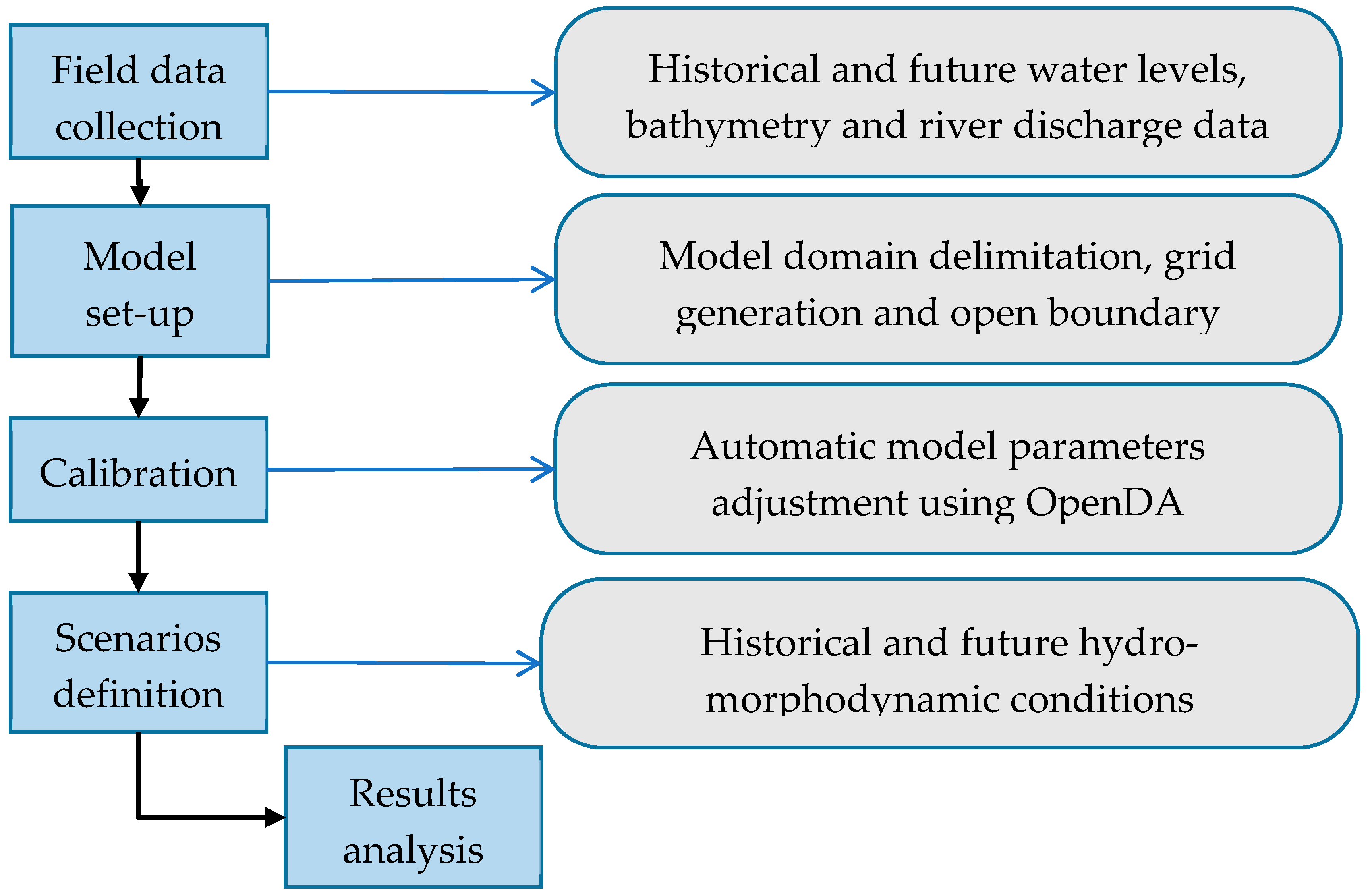
2.2. Methodological Approach

The work methodology comprises five main tasks. Firstly, field data was collected, such as river flow discharges, actual and future coastal water levels, and estuarine bathymetry. Secondly, a numerical model of the estuary was implemented in Delft3D software following usual approaches for hydrodynamic model implementation, for grid generation, and for open boundary conditions specification. A relatively new approach for calibration was implemented. The adopted calibration procedure based on OpenDA, consists of an automatic estimation of the values of some model parameters, aiming to reduce the error between the model results and observed field data. This requires the configuration of some input data specifying the selected calibration algorithm, the model parameters to be calibrated, and the variables to be used to compute the error function. After calibration a sound definition of relevant simulation scenarios was carried out, considering different climate change emissions scenarios combined with different river flood events. Lastly, after running the adopted scenarios the obtained results were judiciously analyzed (Figure 3).

2.3. Numerical Model

The numerical model implemented for the analysis of the hydrodynamic and morphodynamic behavior of the river Minho estuary followed a two-dimensional approach in the horizontal plane (2DH) and was developed using the Delft3D software [12]. This numerical tool solves the Reynolds averaged conservation equations of mass and momentum, being able to simulate hydrodynamic as well as sedimentary transport equations for morphodynamic processes simulation, with satisfactory accuracy, allowing to achieve reliable results [6,11,22].

Estuary delimitation and spatial discretization were supported by Geographic Information System techniques [23]. The model domain was delimited considering all the areas below the elevation of 4.0 m, referred to the Portuguese altimetric datum (MSL) [24]. The fluvial upstream open boundary coincided with a hydrometric station (Foz do Mouro) of the Portuguese Environmental Agency (PEA), which measures water levels with an hourly frequency. The downstream open boundary is located at the Atlantic Ocean at a location of about 80 m depth (MSL).

The model bathymetry was defined based on available bathymetric and topographic data [15]. The model time step was 1 min and, to achieve steady sate solutions, a dynamic simulation time of 24 h was assumed. For bottom friction, a Manning friction law was selected, and the effect of Coriolis acceleration was taken into account assuming the latitude of the estuary (43° N).

The curvilinear grid dimension is 103 × 468 with 20,180 active cells and was generated using the pre-processing tools available for the Delft3D software [25]. The size of the grid cells varies from a minimum cell surface area of 162 m², near the upriver boundary, to a maximum of 26,000 m² at the oceanic boundary. The average cell surface area is 7614 m².

2.4. Automatic Calibration Procedure

The calibration of a numerical model consists of adjusting values of key parameters, aiming to reduce errors between model results and observed data. This is usually a very demanding task in terms of modelling work, involving the realization of numerous simulations, and generating a large amount of data that has to be carefully analyzed to obtain the most accurate results. However, if this procedure is based on automatic procedures supported by optimization tools, less effort is required from the modelers to obtain the best values for the calibration parameters, which minimize model errors [26]. For this purpose, the OpenDA tool was configured and applied.

The OpenDA procedure consists of automatically running the model several times while determining the value of a cost function (Equation (1)) that computes the differences between the observed data and the model results. In each iteration, the software applies increments to the values of the specified parameters and performs a simulation considering the new values. It repeats these steps until it reaches one of the stopping criteria: the maximum number of iterations or the improvement of the error function. At the end of its execution, the program informs which model is considered optimal, that is, the model with the cost function closest to zero. The error function J is given by:

$$J_{\left(x_0\right)}={\displaystyle \sum }_{k=1}^N\left(y^0\left(k\right)-H·x\left(k\right)\right)R^{-1}\left(y^0\left(k\right)-H·x\left(k\right)\right)$$

(1)

where $x_0$ is the initial value of the parameter(s) to be determined,$x\left(k\right)$ is the parameter(s) value at time $k$, $H$ is the observatory operator, $y^0\left(k\right)$ is the observation value at time $k$, $N$ is the total number of time steps, and $R$ is the covariance.

For the model calibration and validation, points were chosen according to the available measured data for the estuary. A specific monitoring campaign [15] involving water level measurements was carried out at six different points in 2006 (points VP1 to VP6 in Figure 1). At the locations of Tui and Goian, coincident with continuous monitoring gauge stations of Galicia, Spain [27], water level measurements for the year 2019 were used. Different calibration strategies, involving different measurement points and periods, were analyzed in order to select the strategy that leads to the minimum cost function. For the 2006 period, the calibration includes two points located at the lower estuary that are relatively close to each other (Figure 1). The second period also includes two points, but one is located at the lower estuary and the other far upstream near Tui.

Calibration parameters include the Manning coefficient values, the tidal constituents M2, S2, N2, and K2, and a uniform correction of the bathymetry. The performance of the model was evaluated by calibrating these parameters individually and simultaneously, considering their variation along different regions of the selected computational domain.

Beside the use of the cost function of the calibration procedure, the performance of the model was assessed computing several statistical error measures for the selected observation points: root mean squared error (RMS), bias (BIAS), and standard deviation (STD).

2.5. Climate Change Scenarios Definition

Model scenarios were defined considering the future evolution of the Minho estuary in the context of climate change. The scenarios correspond to hypothetical/predicted situations that are reflected in different conditions applied at the open boundaries of the model.

River flow discharges were estimated for different return periods, considering the historical data available for the river Minho in the Portuguese river monitoring information system [28]. The peak river flow discharges were estimated using the Gumbel distribution and considering 50 years and 100 years return periods. The expected extreme sea levels (ESL) were extracted from the numerical solutions proposed by Vousdoukas et al. [29], for the location closest to the Minho estuary. These authors performed a numerical forecast for different frequencies of occurrence, based on dynamic simulations of all the major components of extreme sea levels (tide, storm surge, wave set-up, and sea level rise), considering the CMIP5 [30] projections for the Representative Concentration Pathways (RCP) 4.5 and RCP 8.5.

In order to simulate extreme levels along the estuary, the peak river flow discharge scenarios, associated with return periods of 50 years (occurrence probability of 2%) and 100 years (occurrence probability of 1%), were combined with the same ESL return periods estimated for the ocean open boundary. Assuming that these two variables are independent, which is a rough simplification as demonstrated by [31], their combination results in probabilities of 0.04% (return periods of 50 years) and 0.01% (return periods of 100 years). For comparison purposes, the present astronomic tidal water level variations are considered for both neap and spring tides. In S04, S05, S09, and S10 scenarios, with the objective to have a baseline scenario for comparison, we neglected the actual SLR by assuming an ocean boundary water level of 0.0 m (MSL), maintaining all the other components that could contribute to ESL.

Table 1. Climate change hydrodynamic modelling scenarios.

Scenario	Return Period (years)	River Flow (m³/s)	Climate Scenario	Expected ESL (m)	Ocean Boundary Water Level
S01	50	5364.5	Historical	2.9	Constant
S02	50	5364.5	RCP 4.5	3.1	Constant
S03	50	5364.5	RCP 8.5	3.1	Constant
S04	50	5364.5	Historical	0.0	Variable—neap tide
S05	50	5364.5	Historical	0.0	Variable—spring tide
S06	100	6037.7	Historical	3.0	Constant
S07	100	6037.7	RCP 4.5	3.4	Constant
S08	100	6037.7	RCP 8.5	3.6	Constant
S09	100	6037.7	Historical	0.0	Variable—neap tide
S10	100	6037.7	Historical	0.0	Variable—spring tide

summarizes the characteristics of each of the considered scenarios.

Exploratory scenarios were also defined to anticipate possible impacts due to climate change of ESL on the sediment transport patterns within the river Minho estuary. The historic and future scenarios considered for the morphodynamic simulations were similar to those presented in Table 1 for the hydrodynamic simulations. Though an additional scenario was included, considering a more frequent river flow discharge, with a value corresponding to the 85th percentile of the historical river flow time series.

Table 2. Climate change morphodynamic modelling scenarios.

Scenario	Return Period (years)	River Flow (m3/s)	Climate Scenario	Expected ESL (m)	Ocean Boundary Water Level
M01	-	541.05	Historical	0.0	Constant
M02	50	5364.50	Historical	2.9	Constant
M03	50	5364.50	RCP 4.5/RCP 8.5	3.1	Constant
M04	100	6037.70	Historical	3.0	Constant
M05	100	6037.70	RCP 4.5	3.4	Constant
M06	100	6037.70	RCP 8.5	3.6	Constant
M07	-	541.05	Historical	0.0	Variable—neap tide
M08	-	541.05	Historical	0.0	Variable—spring tide

presents the main characteristics of the simulated morphodynamic scenarios.

Due to silting, the artificial navigation canal between Caminha and La Guardia (Figure 2) requires frequent dredging works to maintain its depth and allow navigation without restrictions during low tide conditions. To analyze present and future conditions of accretion at the navigation canal, four different morphodynamic scenarios were defined based on the conditions indicated in Table 2: two steady-state scenarios corresponding to the historic and estimated ESL (FB02 and FB03), another steady state scenario corresponding to a flood event with a return period of 50 years and low tide water level (FB04) and a fourth scenario performing a long-term simulation of 1 year, considering average river flow discharges (FB01), resulting from the application of a morphological scale factor of 52 [12]. This factor accelerates the erosion and accretion processes during the numerical modelling simulation.

Table 3. Scenarios for sedimentation assessment at the Caminha–La Guardia navigation canal.

Scenario	River Flow Discharge Return Period (years)	River Flow m³/s	Morphological Scale Factor	Expected ESL (m)
FB01	-	325.8	52	0.0
FB02	50	5364.5	1	2.90
FB03	100	6037.7	1	3.10
FB04	50	5364.5	1	−1.78

summarizes the characteristics of the scenarios defined to analyze accretion conditions in the navigation canal.

The sediment fraction considered in the morphodynamic simulations presented a D₅₀ (median diameter) of 0.59 mm, as indicated by Balsinha et al. [32], for the FBO1–FBO3 scenarios and a D₅₀ of 0.20 mm for the FBO4 scenario.

3. Results

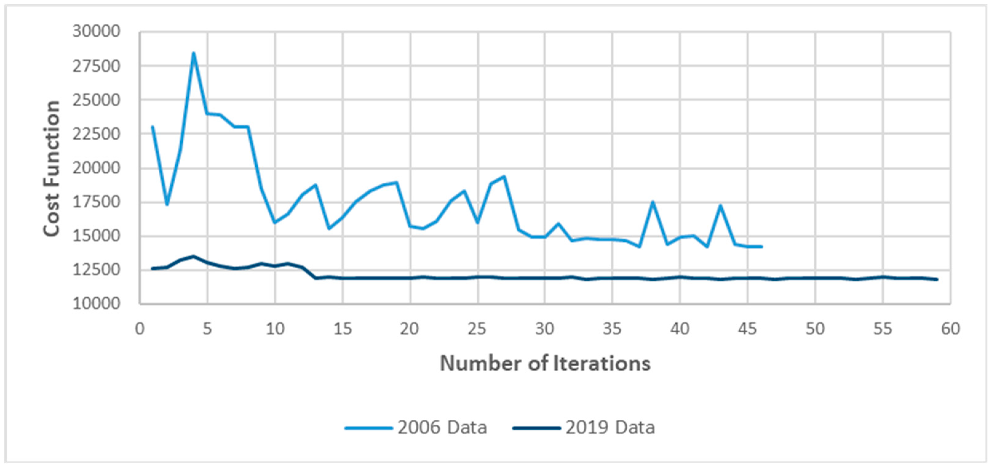
3.1. Model Calibration Results

Calibration error cost function results are presented in Figure 4. These results correspond to a set-up of the OpenDA configuration for the simultaneous calibration of all the specified parameters. Initially, the individual influence of each parameter was assessed, applying a variation according to the initially defined standard deviations. This explains why the cost function increases in the first iterations. After that, all the parameters were allowed to vary in each iteration, until the lowest value of the cost function was achieved.

A statistical summary of the errors for the two calibration periods is presented in

Table 4. Statistical analysis of the calibration results.

Calibration Period	Observation Point	RMS	Mean RMS	Bias	Mean Bias	STD	Mean STD	Cost Function
2006	VP3	0.1846	0.2113	−0.0876	−0.1362	0.1626	0.1563	14,185.44
	VP4	0.2380		−0.1848		0.1501
2019	Tui	0.3385	0.2696	−0.1401	−0.0932	0.3085	0.2520	11,845.64
	Goian	0.2007		−0.0462		0.1955

. Results showed a lower RMS and standard deviation for the 2006 period than for the 2019 period. On the other hand, the bias and the cost function associated with the 2019 data were lower.

Considering that the error cost function and the statistical parameters for both calibration periods were quite similar, the adopted values for the calibration parameters correspond to the ones obtained for the 2019 calibration. The results for this simulation were selected because the in-situ data consist of continuous measurement records, which can be used in future studies and modelling improvements for data assimilation purposes. The final calibration parameters values are presented in

Table 5. Model parameters used in the numerical model.

Parameter	Value	Parameter	Value
M2 amplitude (m)	0.557	K2 amplitude (m)	0.082
M2 phase angle (degrees)	73.953	K2 phase angle (degrees)	102.482
S2 amplitude (m)	0.169	Horizontal eddy viscosity (m2/s)	3.000
S2 phase angle (degrees)	118.549	Upper estuary Manning coefficient (m−1/3·s)	0.019
N2 amplitude (m)	0.178	Lower estuary Manning coefficient (m−1/3·s)	0.026
N2 phase angle (degrees)	55.391

.

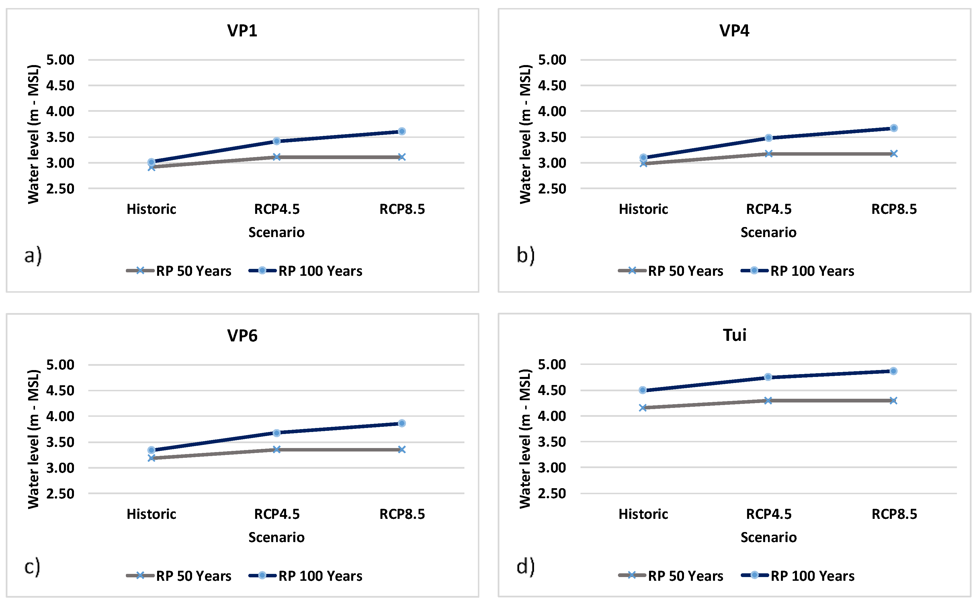
3.2. Hydrodynamic Results

The main results of the simulated water levels are presented in Figure 5 for different extreme sea levels and flood peak discharges (FPD). Water levels within the estuary, downstream of Tui, vary from 2.9 (MSL) to 3.9 m (MSL), considering all the simulated climate change hydrodynamic modelling scenarios. Water levels along the estuary are predicted to rise on average 0.16 m, for the scenarios that considered RCP 4.5 and RCP 8.5 conditions and 50 years return period flood events (S02 and S03 scenarios). Higher water levels were obtained considering the same RCP conditions and river flow discharges associated with 100 years return period flood events. For these scenarios (S07 and S08), the water level is expected to rise 0.32 and 0.48 m for RCP 4.5 and RCP 8.5, respectively.

The Minho estuary is marked by two natural geometric constrictions, one at the estuary mouth and the other near Goian/Vila Nova da Cerveira. These constrictions have a pronounced effect on water level gradients, causing distinct water elevation patterns upstream and downstream of these locations. Upstream of Goian/Vila Nova da Cerveira, the influence of the river is stronger when compared to the lower estuary. Between Goian/Vila Nova da Cerveira and the estuary mouth, the oceanic conditions gain a marked influence on the hydrodynamic behavior, as expected.

Depth averaged velocities are presented in Figure 6. The maximum velocities occur at narrower estuarine sections, including the natural geometric constrictions described above, where strong water level gradients were previously identified. Climate change scenarios imply a slight weakening of the current velocity at those locations, as expected due to the increase in the cross-sectional area associated with the higher water level.

Although tides can suffer some variations due to astronomic influences during this century [33], these variations are not considered in the simulated scenarios. In the proposed numerical simulations, the present tidal constituents with constant values through the years were considered. Results for the two flood events during either spring or neap tides are presented in Figure 7. It is clear that the tidal influence slightly diminishes as the flood peak discharge intensifies, and also that it suffers a strong decline with increasing distance to the estuary mouth. Neap tides are not strong enough to produce a marked effect, even at the most downstream locations, due to the strong river flows imposed in those scenarios. Small differences in the water level elevation between S4 and S9 and between S5 and S10 were observed, probably related to the simulated river flows (5364.5 and 6037.7 m³/s) that strongly reduced the tide amplitude at upriver locations (Tui and VP6).

Additionally, note that minimum water levels within the estuary are higher than ocean levels (not shown) during flood events. This is caused by the narrow estuary mouth, restricting river discharge.

To better represent the changes in the tidal elevation of the performed scenarios, the attenuation of tidal amplitudes along the estuary was computed for different locations (VP4, VP6, and Tui, Figure 1) by comparison to the maximum amplitude at VP1, for both spring and neap tides (scenarios SX and SY). The results, presented in

Table 6. Results for the variation of tidal amplitudes along the Minho estuary.

Scenario	Tidal Amplitude as Percentage of the Amplitude at VP1 (%)
	VP4	VP6	Tui
S04 (Spring tide, flood peak discharge for RP 50 years)	81	49	27
S05 (Neap tide, flood peak discharge for RP 50 years)	81	45	23
S09 (Spring tide, flood peak discharge for RP 100 years)	79	45	23
S10 (Neap tide, flood peak discharge for RP 100 years)	78	42	22

, show that at VP4 the tidal amplitude is about 80% of the tidal amplitude verified at VP1, at VP6 it ranges from 42% to 49%, and at Tui it decreases to a range from 22% to 27%, mainly depending on the river flood peak discharge.

Depth averaged velocity results for a spring and a neap tide are shown in Figure 8. For the simulated river flood peak discharges, currents do not suffer inversion inside the estuary. As expected, the highest velocity magnitudes occur during ebb tide (see also Figure 7), the amplitude of velocity being more significant at downstream locations (VP1, VP2) rather than upriver (VP6, Tui).

Variations of velocity magnitude reach 3 m/s at VP1 and 0.4 m/s at Tui, for spring tides, and are of the order of 1 m/s at VP1 and near nil at Tui, for neap tides.

The impact of climate change in terms of extreme water levels is shown in Figure 9 at four different locations: VP1, VP4, VP6, and Tui. The worsening of the extreme water levels has similar values at VP1 and VP4. At these locations, for the worst scenario (RCP 8.5 and RP 100 years), a 0.6 m increase in water level is predicted. At VP6, this increase will be 0.5 m, and at Tui it will be 0.4 m. For the RCP 4.5 and RP 100 years’ scenarios, the water level increase will be about 0.4 m at VP1 and VP4, 0.3 m at VP6, and 0.2 m at Tui. Results for scenarios involving RP 50 years do not show differences between the two emissions scenarios (RCP 4.5 and RCP 8.5) since, according to [22], the predicted ocean extreme water levels are identical. In this case, the expected water level rises are 0.2 m at VP1, VP4, and VP6, and 0.1 m at Tui.

It was observed that the flooded areas upstream of Vila Nova de Cerveira are quite similar for all the simulated scenarios. Variations in the location of the inundated areas start to appear downstream of this location. However, three areas particularly prone to inundations were identified at the estuary banks, for the worst considered scenario (S8). These regions, in O Río (Spain), Vila Nova da Cerveira (Portugal), and Caminha (Portugal) (Figure 10), are all located at an elevation below 4.0 m (MSL). While in Caminha the flooding could reach a considerable number of urban infrastructures, at O Río the affected area is mostly occupied by rural infrastructures.

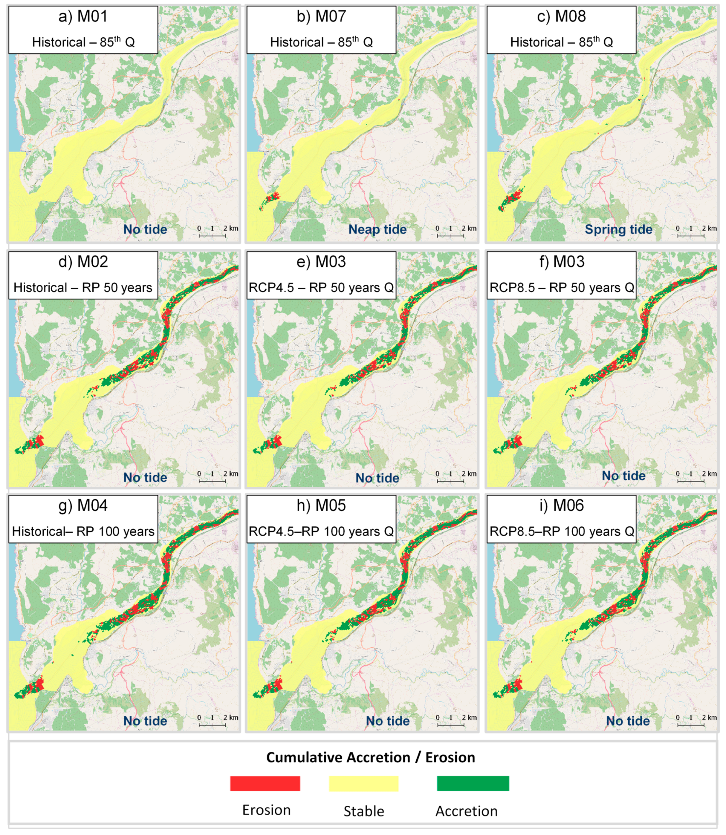
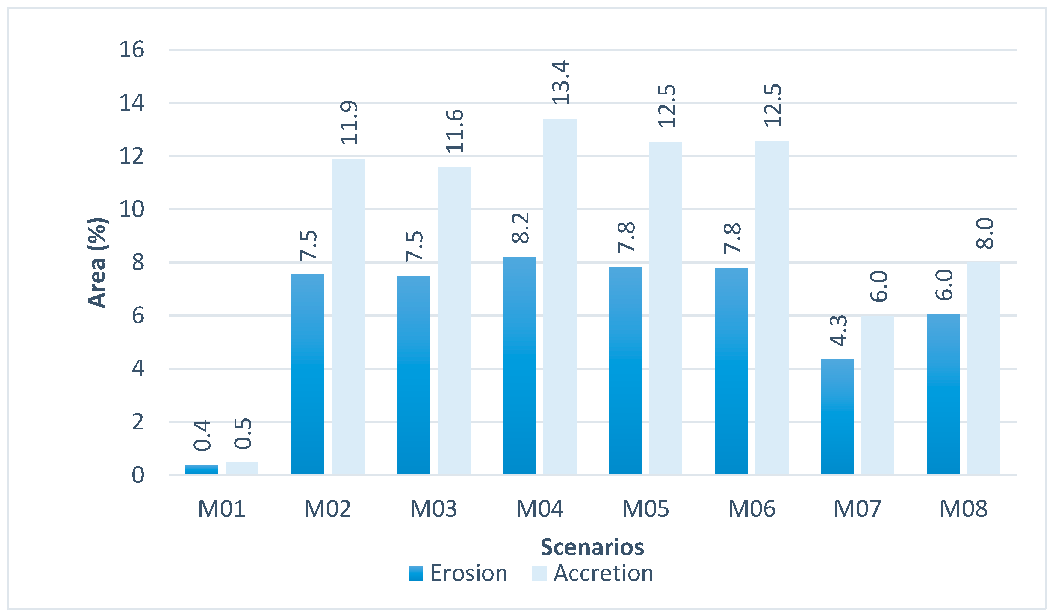
3.3. Morphodynamic Results

The exploratory morphodynamic simulations aimed to characterize the patterns of sediment transport for different conditions of water level and river flow. As there was no data available related to the transport of sediment that occurs in the estuary, the morphodynamic module of the Delf3D model was not calibrated. Thus, the results presented herein, although quantified in terms of cumulative erosion/accretion, were qualitatively interpreted and should be considered with caution. The model solutions show that, for average water level conditions and a river discharge of 541.05 m³/s, the cumulative accretion/erosion for short term periods (daily time) is almost null, despite the tide conditions (Figure 11, scenarios M01, M07, and M08). With this river flow forcing, the morphological changes are restricted to the estuary mouth. However, the cumulative erosion/accretion suffers a strong increase during floods, even when sea level rise conditions are considered.

In terms of climate change, i.e., SLR, impacts on the morphodynamics, the obtained results (scenarios M02 to M06) show that these impacts will be minimal in this estuary (Figure 11). This became evident when the ratios of erosion/accretion areas were computed using Geographic Information Systems (GIS) tools (Figure 12). The results show more accretion than erosion area for all scenarios and reinforce the importance of flood events for the sediment transport within the estuary.

Finally, the conditions of accretion in the navigation canal between Caminha and La Guardia were analyzed. The obtained results (Figure 13) show that there is almost no sediment accumulation under average conditions (FB01). For flood conditions and potential climate change effects (FB02 and FB03) the accretion/erosion is intensified, but the navigation canal is not affected by either erosion or accretion for the relatively coarse simulated sediment sizes (D₅₀ = 0.59 mm). Indeed, if finer sediment is considered (FB04), the sediment transport intensifies along the estuary, and, even in a short period, a flood event can lead to an intense deposition of sediments in the navigation canal.

4. Discussion

The methodological approach supported by OpenDA and used for the calibration of the numerical model revealed its usefulness in reducing the effort needed to perform the modelling set-up. Computationally, it is an efficient tool, rapidly converging to a final solution with an acceptable error, while considering simultaneous estimation of different calibration parameters. The bias analysis demonstrated that both data sets selected from field campaigns and hydrometric gauges for calibration, resulted in a slight underestimation of the water levels. The various sources of uncertainty associated either to the defined extreme ocean water levels [22] or the implemented model forcing functions and parameters, advised a continuous effort in the calibration of the model. An adequate answer to this inherent uncertainty is to turn the model operational [34] and to use assimilation techniques [35], based on continuous monitoring data. Thus, the values of the calibration parameters associated with the second data set (hydrometric gauges) were adopted, allowing the modelled scenarios to be updated as new data and more reliable climate change scenarios become available.

The impact of climate change in terms of water levels within the estuary is nonlinear [26,27]. Indeed, an increase of the present ESL of 2.9 (scenario S01) to 3.6 m (scenario S08) results in different water level rise values along the estuary, considering only the hydrodynamic behavior. Moreover, assuming that the estuarine bathymetry will be the same at the end of the century constitutes a great simplification since either sediment accumulation or marine vegetation will certainly play important roles in the natural estuarine adaptation to SLR [28]. However, the obtained aggravated water levels can be adopted as adequate estimates for coastal planning and for the adoption of structural measures in the context of climate change adaptation, and vulnerability and resilience assessments. It is also expected that, in the context of the extreme water levels analysis, other nonlinear effects can induce changes in water levels and tide propagation inside the estuary, as pointed out by [29,30]. These effects are, however, not relevant during flood events since, for these conditions, the Minho estuary is dominated by river discharges.

Based on the obtained hydrodynamics results, several estuarine areas with high inundation risk were identified. These results could be considered by the responsible entities for flood management as a guide to identify the main critical zones and plan adequate mitigation measures, increasing the resilience of the potentially affected areas against the effects of extreme events, protecting urban areas and reducing human and economic losses.

According the simulated exploratory scenarios, climate change will slightly reduce the sediment transport in average conditions, since the SLR will reduce the current intensities. Although, the increase in the frequency of extreme events (floods) can have a contradictory effect by enhancing the sediment transport. During flood events there is almost no sedimentation/erosion within the estuary for the simulated flood scenarios, and the sediments are mainly transported to the coastal platform.

The morphodynamic results showed that sedimentation processes are predominant over erosion when fine sediments are considered. The found accretion/erosion patterns can be used to determine an optimal location for the navigation channel that connects Caminha and La Guardia, through the identification of estuarine areas that will require less dredging, reducing the channel maintenance costs. Indeed, according to the exploratory simulations results, in its present location, fine sediments are deposited in the navigation channel. Further in-situ data are required to perform the calibration of the sediment transport module and increase the confidence of the morphodynamic numerical models.

The obtained results encourage the realization of smaller-scale studies in the Minho estuary, aiming to study local solutions to the identified problems associated with climate change scenarios. This can be easily achieved using a nesting grids implementation approach. Additionally, it is recommended to extend the use of the OpenDA to the calibration of other model parameters, since it was only used for the water level measurements. This tool can also be used to calibrate parameters based on measurements of velocities, sediment budget salinity, and temperature, modelled in Delft3D. Furthermore, it is also important to improve the uncertainty characterization associated to the occurrence of river flow discharges and sea level rise, which is important for the development of reliable decision support systems.

5. Conclusions

A numerical model of the river Minho estuary was implemented using Delft3D in a pioneering work to assess climate change impacts in this estuary. The developed work constitutes a major contribution to the actual knowledge at this region to anticipate the effects of impacts associated with this phenomenon, such as the SLR. The characterization of extreme events is a challenging task, since these events have a high return period, which implies a significant lack of field data to adequately describe their impacts. The methodology used in the present study proved to be effective in forecasting the impact of climate change in estuarine regions and can be adapted to other estuaries and coastal areas.

The calibration methodology based on the OpenDA tool revealed to be effective to achieve reliable modelling results with minimum modeler’s effort. This task is crucial for a good performance of the numerical model, and the OpenDA helps reducing eventual errors that are usually associated with a manual calibration procedure. This is extremely important, since one of the main difficulties in applying numerical models is the time needed in the calibration task.

Extreme water levels rise for the RCP-RP 50 years’ scenarios are identical, according to the ESL adopted at the ocean open boundary. The rise of water levels for RCP scenarios associated with RP 100 years are nearly 0.5 m, ranging from 0.4 to 0.6 m, depending on the location within the estuary.

The morphodynamic results showed that the main driving factors for the sediment transport occurring in the river Minho estuary either under actual or future climate scenarios are the river flood events, tidal conditions, and sediment sizes. Obtained model results agreed well with results found by Rovira et al. [15], that studied in their work the importance of the floods for sediment transport along the estuary, and identified an erosion area at the mouth of the river and the influence of upstream dams in lowering flood peak discharges.

Finally, this study highlights the importance of numerical models for the understanding of the complex hydro-morphodynamic processes that take place in estuaries. Numerical models allow to reproduce observed hydrodynamic patterns and forecast the expected behavior for hypothetical scenarios. With these tools it is possible to anticipate potential problems and design adequate mitigation solutions. Since long term forecast imply a huge uncertainty for horizons of 50–100 years [36], it is advised to implement operational models that assimilate the historical behavior and continuously produce new forecasts. The costs for the study and for implementing measures to adapt and increase the resilience of sensible areas against these problems will be less than the cost of repairing the damages after the occurrence of extreme events.

References

1. IPCC. Special Report on the Ocean and Cryosphere in a Changing Climate; IPCC: Geneva, Switzerland, 2019. [Google Scholar] [CrossRef] [Green Version]
2. Kopp, R.E.; Kempd, A.C.; Bittermanne, K.; Hortonb, B.P.; Donnellyi, J.P.; Gehrelsj, W.R.; Haya, C.C.; Mitrovicak, J.X.; Morrowa, E.D.; Rahmstorfe, S. Temperature-Driven Global Sea-Level Variability in the Common Era. Proc. Nat. Acad. Sci. USA 2016, 113, E1434–E1441. [Google Scholar] [CrossRef] [PubMed] [Green Version]
3. Dangendorf, S.; Wahl, T.; Hein, H.; Jensen, J.; Mai, S.; Mudersbach, C. Mean Sea Level Variability and Influence of the North Atlantic Oscillation on Long-Term Trends in the German Bight. Water 2012, 4, 170–195. [Google Scholar] [CrossRef]
4. Miranda, L.B.; Castro, B.M.; Kjerfve, B. Principios De Oceanografia Fisica De Estuarios; Editora da Universidade de São Paulo: São Paulo, Brazil, 2012. [Google Scholar]
5. Radović, V.; Iglesias, I. Extreme Weather Events: Definition, Classification and Guidelines towards Vulnerability Reduction and Adaptation Management; Springer: Cham, Switzerland, 2019; pp. 1–13. [Google Scholar] [CrossRef]
6. European Comission. Guidelines on the Implementation of the Birds and Habitats Directives in Estuaries and Coastal Zones; European Comission: Brussels, Belgium, 2012. [Google Scholar] [CrossRef]
7. Fenoglio-Marc, L. Analysis and Representation of Regional Sea-Level Variability from Altimetry and Atmospheric-Oceanic Data. Geophys. J. Int. 2001, 145, 1–18. [Google Scholar] [CrossRef]
8. Iglesias, I.; Lorenzo, M.N.; Lázaro, C.; Fernandes, M.J.; Bastos, L. Sea Level Anomaly in the North Atlantic and Seas around Europe: Long-Term Variability and Response to North Atlantic Teleconnection Patterns. Sci. Total Environ. 2017, 609, 861–874. [Google Scholar] [CrossRef] [PubMed]
9. Nerem, R.S.; Leuliette, É.; Cazenave, A. Present-Day Sea-Level Change: A Review. Comptes Rendus Geosci. 2006, 338, 1077–1083. [Google Scholar] [CrossRef]
10. Karathanasi, F.E.; Belibassakis, K.A. A Cost-Effective Method for Estimating Long-Term Effects of Waves on Beach Erosion with Application to Sitia Bay, Crete. Oceanologia 2019, 61, 276–290. [Google Scholar] [CrossRef]
11. Iglesias, I.; Venâncio, S.; Pinho, J.L.; Avilez-Valente, P.; Vieira, J.M.P. Two Models Solutions for the Douro Estuary: Flood Risk Assessment and Breakwater Effects. Estuaries Coasts 2019, 42, 348–364. [Google Scholar] [CrossRef]
12. Deltares. Delft3D 4 Suite (Structured). Available online: https://www.deltares.nl/en/software/delft3d-4-suite (accessed on 7 February 2019).
13. The OpenDA Association. OpenDA User Documentation. Available online: https://www.openda.org/docu/openda_2.4/doc/OpenDA_documentation.pdf (accessed on 16 June 2020).
14. Leorri, E.; Fatela, F.; Drago, T.; Bradley, S.L.; Moreno, J.; Cearreta, A. Lateglacial and Holocene Coastal Evolution in the Minho Estuary (N Portugal): Implications for Understanding Sea-Level Changes in Atlantic Iberia. Holocene 2013, 23, 353–363. [Google Scholar] [CrossRef]
15. Rovira, A.; Ballinger, R.; Ibáñez, C.; Parker, P.; Dominguez, M.D.; Simon, X.; Lewandowski, A.; Hochfeld, B.; Tudor, M.; Vernaeve, L. Sediment Imbalances and Flooding Risk in European Deltas and Estuaries. J. Soils Sedim. 2014, 14, 1493–1512. [Google Scholar] [CrossRef]
16. Ribeiro, D.C.; Costa, S.; Guilhermino, L. A Framework to Assess the Vulnerability of Estuarine Systems for Use in Ecological Risk Assessment. Ocean Coast. Manag. 2016, 119, 267–277. [Google Scholar] [CrossRef]
17. Iglesias, I.; Avilez-Valente, P.; Bio, A.; Bastos, L. Modelling the Main Hydrodynamic Patterns in Shallow Water Estuaries: The Minho Case Study. Water 2019, 11, 1040. [Google Scholar] [CrossRef] [Green Version]
18. Rio-Barja, F.X.; Rodríguez-Lestegás, F. Os Ríos, in as Augas de Galicia. Cons. Cult. 1996, 178–180. [Google Scholar]
19. Iglesias, I.; Avilez-Valente, P.; Luís Pinho, J.; Bio, A.; Manuel Vieira, J.; Bastos, L.; Veloso-Gomes, F. Numerical Modeling Tools Applied to Estuarine and Coastal Hydrodynamics: A User Perspective. In Coastal and Marine Environments-Physical Processes and Numerical Modelling; IntechOpen: London, UK, 2019. [Google Scholar] [CrossRef] [Green Version]
20. APA, Agência Portuguesa do Ambiente. Plano de Bacia Hidrográfica Do Rio Minho; APA: Amadora, Portugal, 2001. [Google Scholar]
21. Des, M.; DeCastro, M.; Sousa, M.C.; Dias, J.M.; Gómez-Gesteira, M. Hydrodynamics of River Plume Intrusion into an Adjacent Estuary: The Minho River and Ria de Vigo. J. Mar. Syst. 2019, 189, 87–97. [Google Scholar] [CrossRef]
22. Siqueira, A.G.; Fiedler, M.F.M.; Yassuda, E.A. Delft3D Morphological Modeling Downstream of Sergio Motta Reservoir Dam. In IAEG/AEG Annual Meeting Proceedings, San Francisco, California, 2018-Volume 4; Springer: Cham, Switzerland, 2019; p. 4. [Google Scholar] [CrossRef]
23. Team, Q.D. Quantum GIS Geographic Information System. Open Source Geospatial Foundation Project. Available online: http://qgis.osgeo.org2016 (accessed on 30 April 2020).
24. Vasconcelos, M.; Botelho, H.; Kol, H.; Casaca, J. The Portuguese Geodetic Reference Frames. Iberia 1995, 95, 12. [Google Scholar]
25. Hydraulics, D. Delft3D-RGFGRID. Generation and Manipulation of Curvilinear Grids for FLOW and WAVE. In User Manual; WL Delft Hydraulics, (Deltares): Delft, The Netherlands, 2005. [Google Scholar]
26. Vieira, J.M.P.; Pinho, J.L.S.; Dias, N.; Schwanenberg, D.; Van Den Boogaard, H.F.P. Parameter Estimation for Eutrophication Models in Reservoirs. Water Sci. Technol. 2013, 68, 319–327. [Google Scholar] [CrossRef]
27. González-Cao, J.; García-Feal, O.; Fernández-Nóvoa, D.; Domínguez-Alonso, J.M.; Gómez-Gesteira, M. Towards an automatic early warning system of flood hazards based on precipitation forecast: The case of the Miño River (NW Spain). Nat. Hazards Earth Syst. Sci. 2019, 19, 2583–2595. [Google Scholar] [CrossRef] [Green Version]
28. Santos, M.A.; Rodrigues, R.; Correia, F.N. Technical Communication: On the European Water Resources Information Policy. Water Resour. Manag. 1997, 11, 305–322. [Google Scholar] [CrossRef]
29. Vousdoukas, M.I.; Mentaschi, L.; Feyen, L.; Voukouvalas, E. Earth’s Future Extreme Sea Levels on the Rise along Europe’ s Coasts Earth ’ s Future. Earth’s Futur. 2017, 5, 1–20. [Google Scholar] [CrossRef]
30. Stouffer, R.J.; Eyring, V.; Meehl, G.A.; Bony, S.; Senior, C.; Stevens, B.; Taylor, K.E. CMIP5 Scientific Gaps and Recommendations for CMIP6. Bull. Am. Meteorol. Soc. 2017, 98, 95–105. [Google Scholar] [CrossRef]
31. Petroliagkis, T.I.; Voukouvalas, E.; Disperati, J.; Bidlot, J. Joint Probabilities of Storm Surge, Significant Wave Height and River Discharge Components of Coastal Flooding Events. European Commission Technical Reports, Italia. Available online: http//bookshop.Eur.eu/en/joint-probabilities-of-storm-surge-significant-wave-height-and-river-discharge-components-of-coastal-flooding-eventspbLBNA278242016,0KABstXJMAAAEjt5AY4e5L (accessed on 15 April 2020).
32. Balsinha, M.J.; Santos, A.I.; Oliveira, A.T.C.; Alves, A.M.C. Textural Composition of Sediments from Minho and Douro Estuaries (Portugal) and Its Relation with Hydrodynamics. J. Coast. Res. 2009, 56, 1330–1334. [Google Scholar]
33. Ray, R.D.; Foster, G. Future Nuisance Flooding at Boston Caused by Astronomical Tides Alone. Earth’s Futur. 2016, 4, 578–587. [Google Scholar] [CrossRef]
34. Pinho, J.L.S.; Vieira, J.M.P.; Do Carmo, J.S.A. Hydroinformatic Environment for Coastal Waters Hydrodynamics and Water Quality Modelling. Adv. Eng. Softw. 2004, 35, 205–222. [Google Scholar] [CrossRef]
35. Werner, M.; Schellekens, J.; Gijsbers, P.; van Dijk, M.; van den Akker, O.; Heynert, K. The Delft-FEWS Flow Forecasting System. Environ. Model. Softw. 2013, 40, 65–77. [Google Scholar] [CrossRef] [Green Version]
36. Idier, D.; Rohmer, J.; Pedreros, R.; Le Roy, S.; Lambert, J.; Louisor, J.; Le Cozannet, G.; Le Cornec, E. Coastal Flood: A Composite Method for Past Events Characterisation Providing Insights in Past, Present and Future Hazards—Joining Historical, Statistical and Modelling Approaches. Nat. Hazards 2020, 101, 465–501. [Google Scholar] [CrossRef] [Green Version]
Figure 1. River Minho estuary: (a) location, (b) bathymetry, and (c) gauging stations.
Jmse 08 00441 g001
Figure 2. Detail of the numerical grid generated for the Minho estuary and ferry navigation channel.
Jmse 08 00441 g002
Figure 3. Methodological approach schematization.
Jmse 08 00441 g003
Figure 4. Cost function variation during the automatic calibration procedure.
Jmse 08 00441 g004
Figure 5. Water level results for the hydrodynamic scenarios combining different values of extreme sea levels (ESL) and flood peak discharges (FPD): (a) ESL = 2.9 m and FPD = 5364.5 m3/s; (b) ESL = 3.1 m and FPD = 5364.5 m3/s; (c) ESL = 3.1 m and FPD = 5364.5 m3/s; (d) ESL = 3.0 m and FPD = 6037.7 m3/s; (e) ESL = 3.4 m and FPD = 6037.7 m3/s; (f) ESL = 3.6 m and FPD = 6037.7 m3/s.
Jmse 08 00441 g005
Figure 6. Depth average flow velocity results for combinations of ESL and flood peak discharges: (a) ESL = 2.9 m and FPD = 5364.5 m3/s; (b) ESL = 3.1 m and FPD = 5364.5 m3/s; (c) ESL = 3.1 m and FPD = 5364.5 m3/s; (d) ESL = 3.0 m and FPD = 6037.7 m3/s; (e) ESL = 3.4 m and FPD = 6037.7 m3/s; (f) ESL = 3.6 m and FPD = 6037.7 m3/s.
Jmse 08 00441 g006
Figure 7. Tidal water levels variation during extreme flood events at different locations in the estuary (VP1, VP4, VP6, and Tui): (a) spring tide and FPD = 5364.5 m3/s; (b) spring tide and FPD = 6037.7 m3/s; (c) neap tide and FPD = 5364.5 m3/s; (d) neap tide and FPD = 6037.7 m3/s.
Jmse 08 00441 g007
Figure 8. Depth averaged velocity variation during extreme flood events at different locations in the estuary (VP1, VP4, VP6, and Tui): (a) spring tide and FPD = 5364.5 m3/s; (b) spring tide and FPD = 6037.7 m3/s; (c) neap tide and FPD = 5364.5 m3/s; (d) neap tide and FPD = 6037.7 m3/s.
Jmse 08 00441 g008
Figure 9. Results of extreme water levels: (a) at VP1, (b) at VP4, (c) at VP6, and (d) at Tui.
Jmse 08 00441 g009
Figure 10. Potentially flooded high-risk areas for the worst scenario. SP for Spain, PT for Portugal: (a) location of risk areas; (b) risk area at Caminha; (c) risk area at O Rio; and (d) risk area at V.N. Cerveira.
Jmse 08 00441 g010
Figure 11. Morphodynamic cumulative accretion/erosion results for scenarios M01 to M08: (a) no tide, ESL = 0.0 m—historical and FPD = 541.05 m3/s; (b) neap tide, ESL = 0.0 m—historical and FPD = 541.05 m3/s; (c) spring tide, ESL = 0.0 m—historical and FPD = 541.05 m3/s; (d) no tide, ESL = 2.9 m—historical and FPD = 5364.50 m3/s; (e) no tide, ESL = 3.1 m—RCP 4.5 and FPD = 5364.50 m3/s; (f) no tide, ESL = 3.1 m—RCP 8.5 and FPD = 5364.50 m3/s; (g) no tide, ESL = 3.0 m—historical and FPD = 6037.70 m3/s; (h) no tide, ESL = 3.4 m—RCP 4.5 and FPD = 6037.70 m3/s; (i) no tide, ESL = 3.6 m—RCP 8.5 and FPD = 6037.70 m3/s.
Jmse 08 00441 g011
Figure 12. Percentage of areas that suffer erosion/accretion for all morphodynamic scenarios.
Jmse 08 00441 g012
Figure 13. Accumulated erosion and accretion processes for scenarios FB01 to FB04 in and around the navigation canal connecting Caminha to La Guardia: (a) river discharge 325.8 m3/s and ESL = 0.0 m; (b) river discharge 5364.5 m3/s and ESL = 2.9 m; (c) river discharge 6037.7 m3/s and ESL = 3.1 m; (d) river discharge 5364.5 m3/s and ESL = −1.78 m.
Jmse 08 00441 g013