Abstract
Three open source wave models are applied in 2DV to reproduce a large-scale wave flume experiment of bichromatic wave transformations over a steep-sloped dike with a mildly-sloped and very shallow foreshore: (i) the Reynolds-averaged Navier–Stokes equations solver interFoam of OpenFOAM® (OF), (ii) the weakly compressible smoothed particle hydrodynamics model DualSPHysics (DSPH) and (iii) the non-hydrostatic nonlinear shallow water equations model SWASH. An inter-model comparison is performed to determine the (standalone) applicability of the three models for this specific case, which requires the simulation of many processes simultaneously, including wave transformations over the foreshore and wave-structure interactions with the dike, promenade and vertical wall. A qualitative comparison is done based on the time series of the measured quantities along the wave flume, and snapshots of bore interactions on the promenade and impacts on the vertical wall. In addition, model performance and pattern statistics are employed to quantify the model differences. The results show that overall, OF provides the highest model skill, but has the highest computational cost. DSPH is shown to have a reduced model performance, but still comparable to OF and for a lower computational cost. Even though SWASH is a much more simplified model than both OF and DSPH, it is shown to provide very similar results: SWASH exhibits an equal capability to estimate the maximum quasi-static horizontal impact force with the highest computational efficiency, but does have an important model performance decrease compared to OF and DSPH for the force impulse.
1. Introduction
Urban areas situated along low elevation coastal zones need to be protected against wave overtopping and flooding during storm conditions. Moreover, many existing sea dikes protecting such coastal urban areas need to be adapted to be prepared for the effects of sea level rise, which is one of the most challenging problems currently facing coastal communities around the world. A hybrid soft-hard coastal defence system is a promising solution in this context [1]. Such a coastal defence system consists of a soft mildly-sloped—usually nourished—beach that acts as a shallow foreshore to a hard steep-sloped sea dike. In many cases, structures on top of the sea dike (e.g., storm walls and buildings fronted by a promenade) are still in danger of being loaded by overtopping storm waves. In the design of these structures, such wave loading needs to be considered. However, this is a challenging task, because along the cross section of a hybrid beach–dike coastal defence system, storm waves are forced to undergo many transformation processes before they reach the structures on the dike. These hydrodynamic processes include shoaling, wave dissipation by breaking (turbulent bore formation) and bottom friction, energy transfer from the sea/swell or short waves (hereafter SW) to their super- and subharmonics (or long waves: hereafter LW) by nonlinear wave–wave interactions, reflection, wave run-up and overtopping on the dike, bore impact on a wall or building, and finally reflection back towards the sea interacting with incoming bores on the promenade.
Therefore, typically experimental modelling is done for this specific case [2]. However, numerical modelling has become a possibility as well by applying computational fluid dynamics (CFD) techniques. In particular, Gruwez et al. [3] have already shown that numerical modelling with a Reynolds-averaged Navier–Stokes (RANS) model (i.e., interFoam of OpenFOAM®) can provide very similar results to large-scale experiments of overtopped wave impacts on coastal dikes with a very shallow foreshore (i.e., from the WAve LOads on WAlls (WALOWA) project [4]). Yet, such Eulerian numerical methods require often expensive mesh generation and need to implement conservative multi-phase schemes to capture the nonlinearities and rapidly changing geometries. Conversely, meshless schemes can efficiently handle problems characterised by large deformations at interfaces, including moving boundaries and do not require special tracking to detect the free surface. Methods such as smoothed particle hydrodynamics (SPH) [5] and the particle finite element method (PFEM) [6] are examples, of which SPH is the most commonly applied in coastal engineering applications [7]. In SPH, the continuum is replaced by particles, which are calculation nodal points free to move in space according to the governing dynamics laws. Although, differently from Eulerian grid-based methods, multiphase air–water SPH models are still quite scarce and have a high computational cost [8,9]. Several studies on coastal engineering applications based on single-phase SPH have been published during the last decades, for example, wave propagation over a beach [10], solitary waves [11], modelling of surf zone hydrodynamics [12], wave run-up on dikes [13], tsunamis forces [14] and wave forces on vertical walls and storm walls [15,16]. Still, single-phase SPH is also inherently expensive computationally, therefore high-performance computing is required. In particular, graphics processing units (GPUs) are employed to accelerate the computations, as, for example, in GPU-SPH [17] and DualSPHysics [18].
Up to now, it has been assumed that numerical models based on the full Navier–Stokes (NS) equations (i.e., RANS and SPH) are necessary for the current case, particularly for the complex two dimensional vertical (2DV) flows occurring on the dike and promenade in front of the structure (or vertical wall) on top of the dike. However, bores impacting vertical walls have also been modelled before with more simplified numerical models. Overtopped bores propagating over a promenade and impacting a vertical wall show many similarities to tsunami bore impacts on vertical walls. Tsunami bore impacts on vertical walls have been numerically modelled by Xie and Chu [19] using shallow-water-hydraulics (SWH) equations, with a hydrostatic pressure assumption, and have shown results consistent with experiments. The nonlinear shallow water (NLSW) equations have been applied before for the modelling of wave overtopping on steep-sloped impermeable dikes [20] and for violent overtopping of steep-sloped seawalls [21], but the lack of frequency dispersion was identified as the limiting factor to be able to correctly reproduce wave grouping. Beyond simple bore propagation, wave frequency dispersion has been added to the NLSW equations in several ways. One such example is OXBOU, a one-dimensional horizontal (1DH) hybrid Boussinesq-NLSW model [22], in which the Boussinesq equations treat the frequency dispersion prior to wave breaking. Whittaker et al. [23] applied this model for the propagation of a transient focussed wave group, wave breaking, overtopping and loading on an inclined seawall with a steep foreshore. They found that when the hydrodynamic contributions are sufficiently small, the perturbed hydrostatic pressure force gives an accurate approximation to the experimentally measured horizontal force. Another example is SWASH, a non-hydrostatic NLSW equations model, where frequency dispersion is resolved by approximation of the vertical gradient of the non-hydrostatic pressure together with a vertical terrain-following grid in a multi-layer approach [24]. It has been shown to be a very efficient and accurate method for the simulation of wave transformations over a (barred) beach [25], including transfer of wave energy to the LWs [26], and mean overtopping discharge [27] and maximum individual overtopping volume [28] over dikes with a very shallow foreshore. However, SWASH has never been validated before for (overtopped) bore impact loading on vertical walls.
To help identify and highlight the (dis)advantages of different types of numerical models relative to each other, inter-model comparisons are typically performed. Vanneste et al. [29] compared a RANS model (FLOW-3D) with DualSPHysics and SWASH for the application of wave overtopping and impact on a quay wall with berm and storm wall on top. They found a qualitatively good correspondence of the wave overtopping and impact on the storm wall for FLOW-3D and DualSPHysics, without an attempt to assess the hydrostatic pressure result from SWASH. They showed that a one-layer SWASH model was not able to accurately predict the wave overtopping in such a case. Buckley et al. [30] compared SWASH with SWAN [31] and XBeach [32] for application to irregular wave transformations in reef environments, where the formation of LWs was also found to be important and was reproduced by SWASH and XBeach. St-Germain et al. [33] compared DualSPHysics and SWASH for monochromatic wave transformation and overtopping on a dike with a shallow foreshore based on numerical snapshots and included a visual validation of surface elevation time series with a physical experiment. In addition, they made a numerical comparison of an irregular wave case. Both models appeared to give similar results for the bulk parameters. However, their comparison was mostly qualitative and therefore not quantified with model performance statics. Park et al. [34] did a laboratory validation and inter-model comparison of two RANS models: a single-phase model (ANSYS-Fluent) and a two-phase model (IHFOAM, part of the open source CFD toolbox OpenFOAM® [35,36,37]). They investigated non-breaking, impulsive breaking, and broken monochromatic wave interactions with elevated coastal structures, and found that the numerical accuracy of wave shoaling and breaking processes played a key role for the accuracy of the forces and pressures on the structure. Both models provided similarly good results, but validation was again mostly limited to a qualitative visual comparison of time series. One exception was the model performance in terms of force and pressure, which was quantified by calculating a normalised residual impulse of force/pressure. González-Cao et al. [38] both validated and inter-compared DualSPHysics and IHFOAM to experiments of breaking monochromatic waves impacting a vertical sea wall with a hanging horizontal cantilever slab, placed on a steep foreshore. They applied model performance and pattern statistics and showed that both models provide comparable results, with IHFOAM narrowly obtaining higher skill scores for low and medium resolutions, whereas for high spatial resolutions both models provided a similar level of accuracy. Finally, Lashley et al. [39] applied a broad range of wave models, including both SWASH and OpenFOAM®, to irregular wave overtopping on dikes with shallow mildly sloping foreshores (similar to the case considered in this paper). They found that accurate modelling of the LWs was essential to obtain accurate results for the mean overtopping discharge q and that the most computationally expensive model is not always necessary to obtain an accurate result. However, the analysis was strictly limited to the bulk parameters of wave transformation until the dike toe and q, and did not consider time series nor individual wave related events.
Therefore, clearly there is still a lack of literature about inter-model comparisons of numerical wave modelling for the combined processes leading to wave impacts on sea dikes and dike-mounted walls in presence of a very shallow foreshore, which also includes a detailed quantitative analysis based on both model performance and pattern statistics. The main goal of this paper is to investigate which type of numerical model is most accurate and most applicable in practice for the considered case. Three open source wave models are selected for standalone application, each representing one of the most popular in its category: (i) a RANS model (i.e., interFoam of OpenFOAM®), (ii) a weakly compressible SPH model (i.e., DualSPHysics) and (iii) a non-hydrostatic NLSW equations model (i.e., SWASH). We chose to investigate the performance of each model as standalone for the present work in order to provide a detailed overview of model capabilities and limitations applied to wave–structure interaction phenomena in very shallow water conditions. The RANS model is the same one as presented by Gruwez et al. [3], which was validated with large-scale experiments of overtopped wave impacts on coastal dikes with a very shallow foreshore from the WALOWA project [4]. In this paper, the same experiment and RANS model are used as a basis for the inter-model comparison with the (until now untested for this case) DualSPHysics and SWASH models. The analysis is done both (i) qualitatively, based on a comparison of the time series of the main measured parameters and snapshots of bore interactions and impacts on the dike, and (ii) quantitatively, based on model performance and pattern statistics, to critically assesses the performance of all three models to reproduce the large-scale experiment. The computational cost of each numerical model is also evaluated in terms of computational and model setup time. Finally, the results are discussed by comparing to results of the numerical models for the individual processes in other available literature, and the applicability of each numerical model for a design case is investigated.
2. Methods
2.1. Large-Scale Laboratory Experiments
Experimental tests to study overtopped wave loads on walls were undertaken in the Deltares Delta Flume. The model, at Froude length scale 1/4.3, consisted of a sandy foreshore and a concrete sea dike with promenade (Figure 1). On top of the promenade a vertical wall was positioned. The water surface elevation η was measured using wave gauges (WG) positioned over the wave flume and promenade, the horizontal velocity Ux with an electromagnetic current meter (ECM) positioned on the promenade [40], and the horizontal wave impact force Fx and pressures p by load cells (LC) and pressure sensors (PS), respectively. Both bichromatic and irregular wave tests were conducted with active reflection compensation (ARC), of which the repeated bichromatic wave test Bi_02_6 (Table 1) was chosen for the inter-model comparison. The test included mostly plunging breakers on the 1:10 transition slope and spilling breakers on the 1:35 foreshore slope in front of the dike. All other relevant details of the tests and the processing of the experimental data used in this paper for the inter-model comparison are provided by Gruwez et al. [3]. For further information on the experimental model setup, the reader is referred to the work in [4]. The WALOWA experimental dataset is available open access [41].
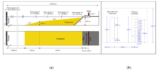
Figure 1.
(a) Overview of the geometrical parameters of the wave flume and WALOWA model setup, with indicated WG locations. Reproduced from the work in [4], with permission from the authors, 2020. (b) Front view of the vertical wall on the promenade with indication of the LCs and PS array.

Table 1.
Hydraulic parameters for the WALOWA bichromatic wave test (EXP) and its repetition (REXP): ho is the offshore water depth, ht the water depth at the dike toe, Hm0,o the incident offshore significant wave height, Rc the dike crest freeboard, fi the SW component frequency, ai the SW component amplitude and δ (=a2/a1) the modulation factor. Reproduced from the work in [3], with permission from the authors, 2020.
2.2. Numerical Models
2.2.1. OpenFOAM
The OpenFOAM® model and model setup as described by Gruwez et al. [3] is used. To summarise, and citing the work in [3], the solver interFoam of OpenFOAM® v6 [42] is applied, “where the advection and sharpness of the water–air interface are handled by the algebraic volume of fluid (VOF) method [43] based on the multidimensional universal limiter with explicit solution (MULES)” [44,45,46]. The boundary conditions for wave generation and absorption are managed by olaFlow [47], while “the turbulence is modelled by the k-ω SST turbulence closure model” that was “stabilised in nearly potential flow regions by Larsen and Fuhrman [48], with their default parameter values [49]”. Hereafter, OF refers to the OpenFOAM® numerical model as presented by the authors of [3].
2.2.2. DualSPHysics
In the present study, DualSPHysics v5.0 [50], based on the weakly compressible SPH method [18], is applied, with the Wendland kernel [51] which controls the interactions between the particles based on a smoothing length hSPH; and with artificial viscosity [52], tuned with parameter αav, which represents the fluid viscosity, prevents particles from interpenetrating, and provides numerical stability for free surface flows [53]. Moreover, employing the artificial viscosity scheme has been shown to exhibit interesting features related to the turbulence field under breaking waves [12]. The weakly compressible SPH method requires that the speed of sound is usually maintained at least 10 times higher than the maximum velocity in the system (managed by the empirical coefficient coeffsound). One consequence is that numerical pressure noise tends to develop [54]. To combat this, a density diffusion term (DDT) was introduced in the continuity equation [54]. This so-called δ-SPH approach increases the smoothness and the accuracy of pressure profiles. The δ-SPH method is applied in this study, by using the improved DDT of Fourtakas et al. [55] where the dynamic density is substituted with the total one. The modified Dynamic Boundary Conditions (mDBC) are employed for the fluid–boundary interactions [56]. Waves are generated by means of moving boundaries that mimic the movement of a laboratory wavemaker. The model also has its own embedded wave generation and absorption system capable for generation of random sea states, monochromatic waves and multiple solitary waves [11,57]. Hereafter, the DualSPHysics numerical model as presented here is simply referred to as DSPH.
The DSPH 2DV model domain extends from the wave paddle, over the foreshore and dike up to the vertical wall on top of the promenade (Figure 2). Some distance behind the vertical wall is also included to allow limited wave or splash overtopping without recirculation of the overtopped water. The boundary of the model domain and vertical wall consists of fixed particles. The water area, bounded by the still water level (SWL) and the fixed bottom, consists of particles that are allowed to move freely according to the SPH governing equations. The particles of the wave paddle move back and forth in the x-direction to reproduce the realised wave piston motion of the experiment including ARC. All fixed or wave paddle prescribed moving particles provide a boundary for the fluid particles according to the mDBC.
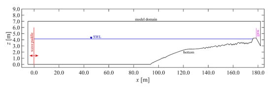
Figure 2.
Definition of the DSPH 2DV computational domain, with coloured indication of the model fixed and movable boundaries. The still water level (SWL) is indicated in blue (z = 4.14 m). Note: The axes are in a distorted scale.
Unlike OF, where a variable grid resolution over the studied domain is used, no likewise or adaptive refinement is implemented in DSPH yet, being still one of the unresolved questions in SPH, also defined within the main SPHERIC Grand Challenges [58]. The resolution in DSPH is determined by the initial particle spacing dp. Previous experience has shown that at least ten particles per regular wave height (i.e., H/dp ≥ 10) are necessary to obtain an accurate regular nonlinear wave profile and propagation [59]. However, to resolve the thin layer flows on the promenade, the water phase particles are assigned an initial particle spacing of dp = 0.02 m, leading to a total of 1,309,056 particles in the model domain. This choice is confirmed by a grid convergence analysis in Appendix A.
All simulations were carried out employing αav = 0.01, which is most commonly used for sea wave modelling [16], and hSPH/dp = 2.12, where the smoothing length is calculated in DSPH according to the initial interparticle distance as hSPH = coefh √2dp in 2DV. In the present calculations, coefh = 1.8 was assumed (usually in the range 1.2 to 1.8 [59]). The recommended and default density diffusion parameter value of 0.1 was chosen. The results of a sensitivity analysis of these parameters showed negligible influence (not shown). The so-calculated kernel size is equal to 0.051 m, which can be considered as the effective model resolution since, citing Lowe et al. (2019), “the kernel size effectively reduces the model resolution by smoothing the results over the length-scale hSPH”. It is therefore twice the finest resolution used on the promenade in the OF model (i.e., dx = dz = 0.0225 m).
The symplectic position Verlet time integrator scheme was employed for time integration, with a variable time step dependent on the Courant–Friedrich–Lewy (CFL = 0.18) condition, the forcing terms and the diffusion term of Monaghan and Kos [10]. The DSPH simulations were run on a NVidia GeForce GTX TITAN Black with 2880 CUDA cores and FP64 (double) performance of 1.882 TFLOPS.
2.2.3. SWASH
In this study, SWASH v5.01 is applied. SWASH (Simulating WAves till SHore) is based on the nonlinear shallow water equations with addition of non-hydrostatic terms. It employs an implementation of the equations of mass and momentum conservation similar to incompressible RANS models, but with a significantly reduced vertical resolution. In the x-direction, the computational domain is discretised in equally sized grid cells and in z-direction the water column is divided into a fixed number of vertical layers K, each with a thickness of Δz = h/K (where h is the local water depth). During wave breaking, SWASH does not model air inclusions and simulates it in a more simplified way, without overturning waves and turbulent vortices, applying a shock-capturing scheme. Moreover, for low vertical resolutions (K < 10), the bore front is approximated in a hydrostatic front approximation (HFA), by analogy of the turbulent bore to a hydraulic jump and by ensuring conservation of mass and momentum [25]. For a complete model description and numerical implementation reference is made to the works in [24,25,26]. Hereafter, the SWASH numerical model as presented here is referred to as SW1L or SW8L depending on the amount of vertical layers K applied (respectively, K = 1 and K = 8).
In SWASH, no boundary condition exists that replicates the wave paddle motion from an experiment. The SWASH 2DV model domain therefore starts at the first experimental wave gauge (i.e., WG02, x = 43.5 m) so that the incident wave time series obtained from a reflection analysis can be applied as a boundary condition for the incident waves. The domain extends further horizontally up to some distance past the top of the vertical wall where overtopped water is allowed to exit the domain (Figure 3). The model domain is vertically bounded by the free surface (z = η(x,t)) and a fixed bottom.
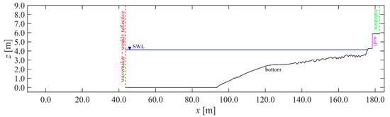
Figure 3.
Definition of the SWASH computational domain, with coloured indication of the model boundaries. The wavemaker and weakly reflective boundary is positioned at the most offshore wave gauge WG02 location (x = 43.5 m). The SWL is indicated in blue (z = 4.14 m). Note: The axes are in a distorted scale.
In the horizontal direction, rectilinear cell sizes are used. For relatively high waves, 100 grid cells per wave length are recommended [60]. The shortest of the two primary components of the bichromatic wave group has a wave length of approximately 30 m (or Δx = 0.30 m) for the water depth at the wave paddle and about 12 m (or Δx = 0.12 m) for the water depth at the toe of the dike. A grid size of 0.2 m is therefore assumed, which is confirmed by a grid convergence analysis in Appendix A. To obtain a correct total water depth in each cell in the vicinity of the steep dike slope and the vertical wall, a bottom level in the cell centres is necessary, which is taken equal to the upper-right corner of each computational cell (by activating BOTCel SHIFT mode in SWASH), thereby preventing errors due to bottom interpolation.
The number of vertical layers is determined by the value of kho (where k is the wavenumber) [61]. For both primary wave components, kho is below 1.0 and a one-layer approach (or depth-averaged, K = 1) is acceptable with respect to frequency dispersion. Although a one-layer approach also appeared to be sufficient in terms of accuracy of water surface elevation for the wave–structure interactions with the dike and vertical wall, a second SWASH simulation was done as well using eight layers (K = 8) to resolve more the flow on top of the dike and in front of the wall. This allows a comparison of the velocity field in the snapshot comparisons with the other two numerical models (Section 3.5) and an evaluation of the model performance of a multi-layer model. Discretisation of the vertical pressure gradient is done by the implicit Keller-box scheme for SW1L, while the explicit central differences layout was applied for SW8L to ensure robustness.
The input at the wavemaker boundary of SWASH is the incident η time series obtained at WG02 by a reflection analysis using the three offshore wave gauges (WG02, 03 and 04), and following the method of Mansard and Funke [62] as it is implemented in WaveLab [63]. Note that the inter-distances of the three wave gauges were not optimised for the considered bichromatic waves, but still the reflection analysis was found to provide a reasonable incident time series. In addition, a calibration factor of 0.95 is applied to the incident surface elevation time series to match the amount of wave energy with the experiment in WG02 (see Section 3.2) introduced into the computational domain. The wavemaker boundary has a weakly reflective boundary condition, which is a numerical active wave absorption system emulating the effects of the experimental ARC. At the outlet boundary past the top of the vertical wall, a Sommerfeld radiation condition is applied, which allows overtopped water to leave the domain. A Manning’s roughness coefficient n value of 0.019 is applied for the entire domain (default value [61]), for both the sand bottom and dike.
2.3. Data Sampling and Processing
Data sampling and processing of the OF model results and synchronisation of the numerical results to the experimental data were discussed by Gruwez et al. [3] and remain valid here. The same methods were applied to the DSPH and SW1L/SW8L model results. Of interest to repeat here is that a 3rd-order Butterworth low-pass filter with a cut-off frequency of 6.22 Hz (i.e., 3.0 Hz at prototype scale which is larger than the natural frequency of 1.0 Hz of typical buildings along the Belgian coast) was applied to the Fx and p time series of both the experiment and numerical model results. This removed the high frequency oscillations caused by stochastic processes during dynamic or impulsive impacts, so that the experimental signal can be reproduced by the deterministic numerical models [3,64].
For the water surface elevation measurement, both the OF and DSPH methods have uncertainties in a breaking region, where the free surface is complex and air/void inclusions are present. However, experimental instruments, such as the resistive wave gauges applied here, can suffer from similar uncertainties [3,12]. In the case of SW1L/SW8L, no air or void inclusions are modelled and η is available explicitly from the governing equations.
The pressure was sampled in OF at the PS locations along the vertical wall, while Fx was calculated by integration of p along the height of the LC (by using the OpenFOAM® library “libforces.so”). In DSPH, p is calculated by interpolating the fluid particle pressure at a distance from the wall equal to hSPH and forces are calculated as the summation of the acceleration values (solving the momentum equation) multiplied by the mass of each boundary particle belonging to the vertical wall. In SWASH, the total pressure, including both the hydrostatic and non-hydrostatic pressures, exhibited strong oscillations in the grid cells closest to the vertical wall (not shown). Contrary to OF and DSPH, the (numerical noise) oscillations were not removed completely by the applied filtering, with significant residual—and in some cases even exacerbated—spurious oscillations. No immediate explanation was found to their root cause. In any case, it was found that these oscillations are attributable to the non-hydrostatic part of the pressure. Therefore, they disappeared entirely when only considering the hydrostatic pressure. The SW1L/SW8L p and Fx time series are therefore limited to the hydrostatic part in further analyses. For SW1L, the hydrostatic pressures at the pressure sensor locations were then calculated by ρg(η-zPS), where ρ is the water density (1000 kg/m3), g the gravitational acceleration (9.81 m/s2), η is taken from the grid cell closest to the vertical wall (which represents most closely the bore run-up height against the vertical wall) and zPS is the z-coordinate of the considered pressure sensor. For SW8L, the hydrostatic pressure was interpolated between the 8 vertical grid cell values closest to the PS locations. The horizontal impact force Fx was obtained by integration of the hydrostatic pressure along the vertical wall.
Furthermore, citing the work in [3], “to investigate the model performance for the SW and LW components separately, the η time series were separated into ηSW and ηLW by applying a 3rd order Butterworth high- and low-pass filter, respectively. A separation frequency of 0.09 Hz was employed, which is in between the bound long wave frequency (f1 − f2 = 0.035 Hz) and the lowest frequency of the primary wave components (f2 = 0.155 Hz).”
2.4. Inter-Model Comparison Method
The inter-model comparison is done qualitatively by comparing the time series of the main measured parameters between the numerical model results and the experimental data. The same model performance and pattern statistics used in the detailed OF model validation by Gruwez et al. [3] (Appendix B) are applied here for the quantitative model performance of DSPH and SW1L/SW8L and the numerical inter-model comparison.
For easier and faster selection of the best model performance between different models, pattern statistics can be visualised in one graph. The Taylor diagram [65] is such an example, which makes use of the relation between the normalised standard deviation (Equation (A9)), the correlation coefficient R (Equation (A11)) and the root mean square error (RMSE). While this diagram allows a straightforward comparison of the performance for amplitude (represented by ) and phase (represented by R) between different models, no information about the bias is provided. Moreover, the Taylor diagram relies heavily on the (centred) RMSE, which is known to be misleading, because it is biased by extremes or outliers in the dataset and is dependent on the data sample size [66]. Minimising the RMSE therefore does not always lead to an improved model performance [67]. Alternatively, Jolliff et al. [67] therefore proposed a skill target diagram, based on the normalised bias B* (Equation (A10)) and the model skill score S:
which has a scale between 0 and 1 (lower values present a better model prediction), and allows to independently move and R closer to 1. In a skill target diagram, B* is taken as the Y-axis of the target diagram and as the X-axis, with being the sign of the standard deviation difference:
Positive and negative X-axis values therefore indicate respectively a higher or a lower standard deviation (or wave height when the considered variable is η) of the modelled time series compared to the observed time series. The closer the model point is to the diagram origin, the better the model performance is to represent the observation. The total model skill score based on this diagram can then be summarised as the distance ST from the origin of the target diagram or
which is bounded by [0, 1]. The closer ST is to zero, the better the skill of the model is to reproduce the pattern of the experimental measurements. The main advantages of a skill target diagram are that it clearly visualises the pattern statistics, and that it provides more insight into different aspects of the model performance than a general numerical model performance statistic, such as Willmott’s refined index of agreement dr (Equation (A5)).
So far, none of the statistics mentioned provide specific information on the model performance of the peak forces and duration of the wave-induced force on the vertical wall. However, both are of high significance to structural damage [68], and their model performance should be assessed as well. The model performance to reproduce the experimental peak forces of each independent wave impact event during the test is evaluated by a dr-value between predicted and observed maximum horizontal force per impact event Fx,max (i.e., dr,Fx,max). The duration of the wave impact can be evaluated by the impulse of the total horizontal force I:
where tN is the total duration of the test. To evaluate the model performance, a normalised predicted impulse is considered:
where Ip and Io are the predicted and observed force impulses calculated by Equation (4), respectively. The observed total horizontal force impulse is overestimated, equal to or underestimated by the prediction when I* > 1, I* = 1 or I* < 0, respectively. Note that I* is evaluated for the complete Fx time series, so that phase differences are disregarded by this parameter. Therefore, I* purely evaluates the correspondence of the total impulse on the vertical wall during the complete test.
3. Results
3.1. Time Series Comparison
The three numerical model results are first compared qualitatively in the time domain to each other and to EXP. For the sake of brevity, not all measured locations, but a selection of sensor locations is presented here. Sensor locations were selected to be representative for different areas along the flume with clearly different physical behaviours of the waves. In Figure 4, the time series of η are compared at measurement location WG04, representing the offshore waves between the wave paddle and foreshore toe; WG07, representing the wave shoaling and incipient breaking area; WG13, representing the surf zone; WG14, representing the inner surf zone and toe of the dike location; and WLDM02, representing the bore interaction area on the promenade. For clarity, the ηLW time series are shown separately in Figure 5. The time series of Ux are compared in Figure 6 at the ECM location on the promenade. For the numerical models, actually the depth-averaged horizontal velocity is shown instead, as it was shown to deliver a better correspondence to EXP than Ux for OF [3]. The same was found to be the case for DSPH (not shown), and SW1L only provides , since it is a depth-averaged model. In Figure 7, the time series of Fx are compared to the LC measurements, and in Figure 8 the time series of p are compared at the PS locations selected at approximately equidistant positions along the array (i.e., 0.28 m from PS01 up to PS09 and 0.24 m up to PS13).
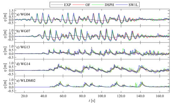
Figure 4.
Comparison of the η time series at selected sensor locations (a–e). The zero-reference is the SWL for panels (a–d) and the promenade bottom for panel (e). Note: ηLW is shown as well, but only for EXP (bold dotted lines in panels (a–d)). Adapted from the work in [3], with permission from the authors, 2020.
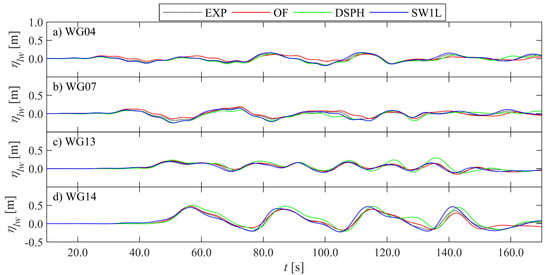
Figure 5.
Comparison of the ηLW time series at selected sensor locations (a–d). The zero-reference is the SWL. Adapted from the work in [3], with permission from the authors, 2020.
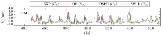
Figure 6.
Comparison of the Ux time series at the ECM location. The zero-reference is the promenade bottom. Adapted from the work in [3], with permission from the authors, 2020.
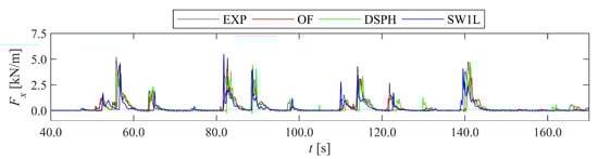
Figure 7.
Comparison of the Fx time series at the vertical wall. The experiment is the load cell force measurement. Adapted from the work in [3], with permission from the authors, 2020.
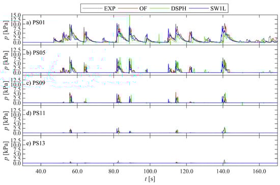
Figure 8.
Comparison of the p time series at selected sensor locations (a–e), PS01 being the bottom PS (a) and PS13 the top-most PS (e). Adapted from the work in [3], with permission from the authors, 2020.
From these figures, it is immediately clear that all three numerical models provide results that are very close to EXP. Especially for η, differences appear to be very small with more significant differences in the surf zone (Figure 4c,d) and on top of the dike (Figure 4e). Further differences are revealed when comparing the η time series of the LW components only. OF does not correspond as well to EXP in the offshore zone (Figure 5a) compared to the other two numerical models. In the surf zone, however, OF shows better correspondence to EXP together with SW1L, while DSPH starts to diverge more from EXP for t greater than approximately 120 s (Figure 5c,d).
Reproducing Ux appears to be more challenging than η for all numerical models. Most of the positive Ux peak values (i.e., flow towards the vertical wall) are reproduced, while some of the return flow durations (i.e., t for Ux < 0) are modelled longer by OF than SW1L, with DSPH being in between (Figure 6). Unfortunately, return flow velocities were often not captured by the ECM measurements in EXP, mostly by too thin flow layers (no data).
For the Fx (Figure 7) and p time series (Figure 8), differences become more distinctive. DSPH shows (small) negative or sub-atmospheric p peaks, not observed in EXP, that occur before some of the dynamic impact peaks and mostly for the lowest PSs (Figure 8a). Both OF and DSPH appear to underestimate most peak values for both Fx and p, while phase differences with EXP are most apparent for DSPH and SW1L.
3.2. Spatial Distribution of Wave Characteristics
The evolution of the root mean square wave height Hrms, the SW and LW components (i.e., Hrms,sw and Hrms,lw), and the mean surface elevation (wave setup) over the wave flume up to the toe of the dike are compared in Figure 9. All models agree on the general evolution of the Hrms curves along the flume. The wave height slightly decreases from the wave paddle up to the toe of the foreshore, more so in case of OF than DSPH (with DSPH closest to EXP): from the wave paddle location to the foreshore toe, Hrms decreases about 10% more for OF than DSPH. SW1L shows a similar behaviour from its offshore boundary (i.e., at WG02) until the foreshore toe and corresponds most with DSPH. On the other hand, SW shoaling is overestimated by both DSPH and SW1L (Hrms,sw at WG07 in Figure 9). In the surf zone, DSPH reproduces the energy loss due to SW breaking best of all three numerical models (i.e., closest result to (R)EXP for Hrms,sw at WG13 and WG14 in Figure 9), while SW1L overestimates and OF underestimates Hrms,sw there.
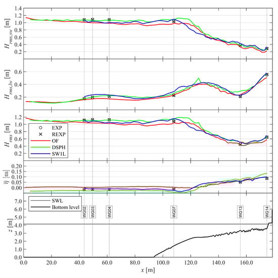
Figure 9.
Comparison of the root mean square wave height Hrms between each numerical model and the (repeated) experiment up to the toe of the dike. From top to bottom: Hrms,sw for the short wave components, Hrms,lw for the long wave components, Hrms for the total surface elevation, mean surface elevation or wave setup and an overview of the sensor locations, SWL and bottom profile. Adapted from the work in [3], with permission from the authors, 2020.
The LW wave height Hrms,lw evolution along the flume in the experiment is also reproduced by all three numerical models. An unexpected peak appears in the DSPH result near x = 126 m, which is not found in the results by OF and SW1L. Moreover DSPH significantly overestimates Hrms,lw at WG13, while OF underestimates Hrms,lw at the dike toe (WG14).
Overall, DSPH provides the best correspondence with (R)EXP for Hrms followed by SW1L, while OF clearly underestimates it for all measured locations. In terms of the wave setup , however, SW1L shows the best correspondence with (R)EXP, while OF and DSPH, respectively, over- and underestimate it until at least WG07. In the inner surf zone, OF corresponds better with (R)EXP for together with SW1L, while DSPH significantly overestimates it ( at WG13–14 in Figure 9).
3.3. Model Performance and Pattern Statistics
More than a qualitative validation and evaluation of inter-model performance is not possible with the time series comparison of Section 3.1, especially when visually almost no discernible and consistent trends of distinction between the model results can be made. The model performance and pattern statistics, provided in Appendix B and Section 2.4, then become very useful for a quantitative evaluation. As dr provides a single dimensionless measure of average error, it is suitable to provide insight into the spatial variation of model error in the flume. In addition to the dr of each numerical model, the dr of the repeated experiment (REXP) is also included in this analysis. A numerical model dr higher than the dr of REXP means that the numerical error cannot be reduced further compared to the experimental repeatability error and a near “perfect” model performance would be achieved with regard to the experiment [3]. Therefore, a relative refined index of agreement d’r (Equation (A8)) and a corresponding rating (Table A1) was defined by Gruwez et al. [3] which provides the performance of the numerical model relative to the experimental model uncertainty. Table 2 and Table 3 provide the dr-values and the pattern statistics at key locations (dike toe and on the promenade, respectively). It is noted that the statistics for η reported in Table 3 were averaged over the four measured locations (WLDM01—WLDM04), for the sake of brevity and because it better represents the statistics for the processes on the promenade. The evolution of dr and R at the WG locations along the wave flume up to the toe of the dike is shown, respectively, in Figure 10 and Figure 11, for ηSW (dr,sw and Rsw), for ηLW (dr,lw and Rlw) and for η (dr,tot and R), and of dr for η and Ux on the dike in Figure 12.
Table 2.
Model performance and pattern statistics evaluated for η of REXP, OF, DSPH, SW1L and SW8L at measured location WG14 (dike toe location). Adapted from the work in [3], with permission from the authors, 2020.
Table 3.
Model performance and pattern statistics evaluated for η of REXP, OF, DSPH, SW1L and SW8L averaged over all measured locations on the promenade (WLDM01—WLDM04) and for Ux at the measured location ECM. Adapted from the work in [3], with permission from the authors, 2020.
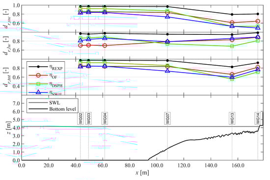
Figure 10.
Comparison of dr, evaluated for REXP, OF, DSPH and SW1L with reference to EXP, up to the toe of the dike. From top to bottom: dr,sw for ηSW, dr,lw for ηLW, dr,tot for η, and finally an overview of the sensor locations, SWL, and bottom profile. Adapted from the work in [3], with permission from the authors, 2020.
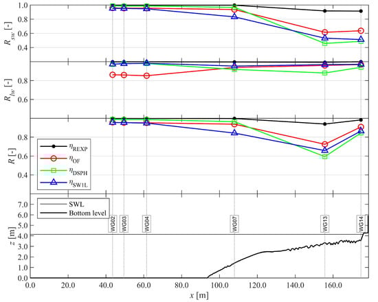
Figure 11.
Comparison of R evaluated for η (of REXP, OF, DSPH and SW1L with reference to EXP) up to the dike toe. From top to bottom: Rsw for ηSW, Rlw for ηLW, R for η, and finally an overview of the sensor locations, SWL, and bottom profile. Adapted from the work in [3], with permission from the authors, 2020.
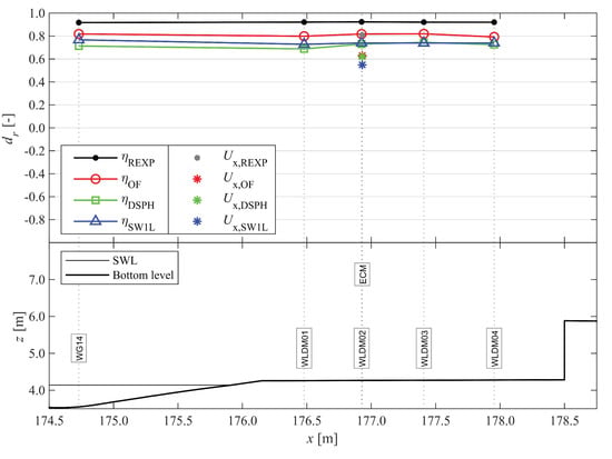
Figure 12.
Comparison of dr, evaluated for η and Ux (of REXP, OF, DSPH and SW1L with reference to EXP) from the toe of the dike up to the vertical wall. From top to bottom: dr for η and Ux, and finally an overview of the sensor locations, SWL, and bottom profile. Adapted from the work in [3], with permission from the authors, 2020.
Offshore, DSPH has the best model performance (WG02-04 in Figure 10, rated Excellent) followed by OF (rated Very Good), and this continues to be so up to the shoaling zone (WG07), although the rating for DSPH drops slightly to Very Good. On the other hand, while SW1L starts offshore with a (relative) model performance similar to OF (rated Very Good), a notable decrease in (relative) model performance occurs in the shoaling zone (WG07, rated Good). All models show a generally decreasing trend of dr,tot over the surf zone (WG07-13) and increases back up to the dike toe (WG13-14). Over the surf zone, DSPH gradually becomes the least performing numerical model (WG13-14, rated Good) followed by SW1L (WG13, rated Good). The relative model performance of SW1L increases back to Very Good at the dike toe (WG14). The performance of OF is not as good as DSPH in the offshore area (WG02-04), but becomes the highest of all three numerical models in the surf zone (WG13-14, rated Very Good) and continues to perform the best on the dike as well (Figure 12), where the dr of η remains more or less constant for all models, with exception of DSPH which increases slightly back to a rating of Very Good.
Separating η into the SW and LW components reveals that dr,sw mostly follows the same trend as dr,tot, with the exception that DSPH performs better than SW1L at the dike toe for dr,sw (Figure 10). On the other hand, dr,lw clearly has a different behaviour: OF does not reproduce the incident LWs as good as DSPH and SW1L, but its LW performance steadily increases towards the dike toe (Figure 10), where the LW energy increases (Figure 9). SW1L shows the overall best LW performance as it shows similar dr,lw values offshore to DSPH and similar values to OF in the surf zone. It is also revealed that the increase in SW1L error at WG07 is mostly caused by a decrease in ηsw performance. Even though SW1L shows the least performance in modelling ηsw over the foreshore, that does not seem to affect its capability of reproducing the LW shoaling and energy transfer from the SW to LW components, with a similar accuracy to OF for modelling ηlw in the surf zone. Increased accuracy of SWASH of the SW modelling can be obtained however, with increased vertical resolution: the SW8L model exhibits much better performance in the shoaling zone (i.e., SW1L: dr,sw,WG07 = 0.73, SW8L: dr,sw,WG07 = 0.86, not shown), and attains the same model performance for η at the toe of the dike as DSPH (dr,sw,WG14 = 0.53). However, because of the smaller wave height of the SW components at the dike toe compared to the LW components (Figure 9), this improvement only slightly increases the overall model performance at the dike toe (Table 2, SW1L: dr,sw,WG14 = 0.85, SW8L: dr,sw,WG14 = 0.86).
The pattern statistics B* and in Table 2 represent, respectively, the accuracy of the wave setup and wave amplitude at the toe of the dike [3], and spatial information of these errors could already be derived implicitly from the and Hrms graphs in Figure 9. Both were already discussed in Section 3.2. The result is that at the toe of the dike, DSPH has the best result of the three numerical models in terms of reproduction of the wave height (Table 2, = 1.02), but the worst result in terms of the wave setup (Table 2, B* = 0.21). OF has the worst result for the wave height (Table 2, = 0.89), while delivering a close second-best result with SW1L for the wave setup (Table 2, B* = 0.05). SW1L provides the lowest wave setup error (Table 2, B* = 0.04).
However, in the previous, spatial information about the accuracy of the wave phase modelling is missing and is shown separately in Figure 11. From this figure it is clear that DSPH introduces the largest error in wave phases over the surf zone up to the dike toe, and that the error is mostly due to phase errors in the SWs. Additionally, an important contribution of phase error is present in the ηLW result of DSPH as well, which is not observed in the other numerical model results. Consequently, at the toe of the dike the phase error is largest for DSPH (i.e., lowest R value in Table 2). However, at the dike toe the difference with SW1L is small, while OF provides the best phase correspondence with EXP.
On top of the dike, the dr of Ux is provided in Figure 12 and Table 3, and indicates a lower model performance for all three numerical models than obtained for η. However, for the relative model performance d’r this difference significantly reduces, so that the same rating is obtained for Ux as for η in case of DSPH and OF (Table 3, rated Very Good). SW1L (and SW8L) has the lowest d’r for Ux and rating (Table 3, rated Good). Although the wave setup at the dike toe is overestimated by each numerical model (Table 2, B* > 0), η on the promenade is generally underestimated and Ux as well (Table 3, B* < 0). The bore wave height is best represented by OF (indicated by ), closely followed by DSPH and SW1L. Phase differences are observed for all numerical models (i.e., R < 1.00 in Table 3), but are lowest for OF, followed by DSPH and SW1L.
Next the dr-values of the pressures at the vertical wall are compared in Figure 13 and the statistics in Table 4. Again, all models show a lower model performance than REXP, and OF obtained the highest value followed by SW1L and DSPH, both of which have very similar model performance along the PS array. Model performances of all models tend to decrease and converge to each other towards higher sensor locations on the vertical wall.
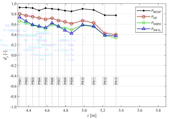
Figure 13.
Comparison of dr evaluated for p (of REXP, OF, DSPH and SW1L with reference to EXP) at the vertical wall (horizontal axis). Adapted from the work in [3], with permission from the authors, 2020.
Table 4.
Model performance and pattern statistics evaluated for p and Fx of REXP, OF, DSPH, SW1L and SW8L at the respective measured locations PS05 and LC. Adapted from the work in [3], with permission from the authors, 2020.
The dr value of Fx for each model is shown in an overview table (Table 4) together with the other pressure and force related statistics. Even though OF has the highest model performance in terms of the Fx time series (Table 4, dr,Fx = 0.76), the force peaks are better estimated by SW1L (Table 4, dr,Fx,max,OF = 0.85 and dr,Fx,max,SW1L = 0.88), while it has the largest errors in the Fx time series (Table 4, dr,Fx = 0.64). Moreover, SW1L underestimates the total impulse much more than OF does (Table 4, I*OF = 0.85 and I*SW1L = 0.62). DSPH has a similar model performance as OF for the force peaks Fx,max, while I* is in between OF and SW1L and its overall model performance for Fx is similar to SW1L. Consequently, the relative model performance for Fx is rated Very Good for OF and Good for DSPH and SW1L. While the model performance slightly increases for SW8L compared to SW1L at the dike toe (Table 2) and on the promenade (Table 3), this does not translate into a better model performance for the wave impact on the vertical wall; in fact, almost every Fx statistic is lower for SW8L than for SW1L (Table 4).
Pattern statistics (B*, and R) are included as well in Table 4. They indicate that all numerical models underestimate the wave impact force and exhibit phase differences. OF shows the least overall underestimation (i.e., B* closest to zero) and the least phase differences (i.e., highest R), while DSPH has the highest value. The results for Fx are slightly worse for the multi-layer model SW8L compared to the single layer model SW1L, except for .
3.4. Skill Target Diagrams
After the spatial inter-model comparisons of Section 3.1, Section 3.2 and Section 3.3 based on the model performance and pattern statistics, the pattern statistics are visualised here together in a skill target diagram as described in Section 2.4 (Figure 14). The selection of observed locations that is considered for these diagrams, is the same as that for the time series plots (Section 3.1). This is to prevent as much as possible a biased evaluation of the model skill in the target diagram, because a particular area had more sensors (i.e., the offshore area for η and the lower half of the pressure sensor array for p). One exception is η on the promenade, for which the pattern statistics were averaged over the four measured locations (WLDM01–WLDM04), and therefore the values from Table 3 are used here as well. The general model performance is visualised by a circle with a radius equal to the mean of the ST skill scores (Equation (3)) or distances from the origin of each model data point in the target diagram of either η (Figure 14a) or p (Figure 14b). The repeated experiment (REXP) is visualised in the skill target diagrams as well, but only by the mean skill circle for η and p. This circle is included to have a reference of the experimental repeatability error. For both Ux and Fx only one representative observed location is available. They are visualised as pentagrams together with the model data points for η and p, respectively.
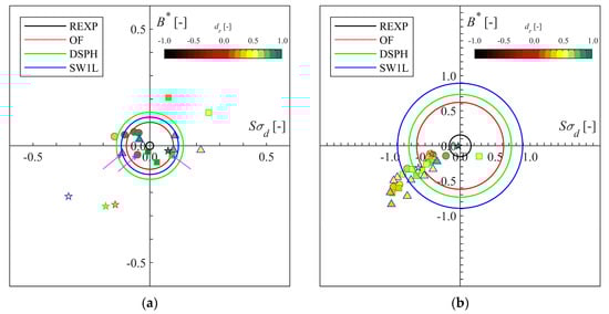
Figure 14.
Numerical model skill target diagrams (target: EXP) for selected sensor locations along the flume. All markers are colour-filled according to the dr colour scale. The circles represent the mean value of all markers for a specific model. The data points of REXP are not plotted for clarity, but only the mean (black circle). (a) Target diagram with pattern statistics for η at locations WG04, 07, 13, 14 and averaged pattern statistics over WLDM01-WLDM04 for the promenade (OF: circles, DSPH: squares; and SW1L: triangles) and Ux at the ECM location (pentagrams). The magenta arrows indicate the markers representing the model performance of η on the promenade (WLDM02). (b) p at approx. equidistant locations PS01, 03, 05, 07, 09, 10–13 (OF: circles, DSPH: squares; and SW1L: triangles) and Fx (pentagrams). Note: the target diagrams have different axis ranges.
None of the mean skill circles of the three numerical models have a smaller radius than the REXP circle, which means that none of the models has an ideal model skill relative to the experimental repeatability. In case of η, the model skill circle of DSPH is largest, and therefore DSPH has the lowest overall model skill, followed by the smaller circles of SW1L and OF (highest model skill), respectively. However, the Ux pentagrams suggest a better Ux model skill of DSPH than SW1L. For p, OF remains the numerical model with the highest model skill, followed by DSPH and SW1L. The Fx pentagrams have the same ranking.
In the η skill target diagram, the numerical model skill for the location on the dike is indicated by an arrow. The remaining numerical model skill scores are those of the measured locations along the flume up to the dike toe. For OF, they are positioned in the top left quadrant, which means that the wave energy is underestimated ( < 0) and the wave setup is slightly overestimated (B* > 0) (both confirmed by Figure 9). For DSPH, the wave energy is mostly overestimated ( > 0). The two points furthest removed from the origin are the measured locations in the surf zone (i.e., WG13-14), where high B* and low R-values (or wave phase differences) are the largest contributors to the decreased DSPH model skill in this area. SW1L generally shows an overestimation of the wave energy ( > 0) and increased wave phase differences (lower R) in the shoaling and surf zones. Generally, SW1L has the best wave setup results (lowest B* values). The Ux skill of all numerical models is one of a clear underestimation (pentagrams in lower left quadrant), of both the mean value (B* < 0) and standard deviation ( < 0), and increased phase difference (low R-values). The same is valid for p and Fx, where all numerical model skill points are also positioned in the lower left quadrant.
3.5. Snapshot Inter-Model Comparison
The numerical models applied in this paper typically have a higher spatial resolution of the physical parameters of interest (e.g., η, U, p) than an experiment. This allows a comparison of snapshots between the numerical models. To allow a comparison of the velocity field, the multi-layered model SW8L is used instead of SW1L. The first main impact series is most appropriate for such a comparison, because accumulation of errors is lowest at the beginning of the test. Snapshots of the flow on the dike and the pressure distribution along the vertical wall are compared in Figure 15, Figure 16 and Figure 17. A few key time instants in the Fx and Ux time series were selected during this series of impacts and are listed chronologically in Table 5. These time instants were selected from each model result independent of time, because due to phase errors these key time instants have occurred at (slightly) different times between the models.
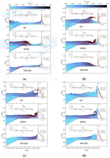
Figure 15.
Numerical comparative snapshots of the water flow on the dike. Colours are the velocity magnitude |U| according to the colour scale shown at the top of each figure. The red arrows are the velocity vectors, which are scaled for a clear visualisation. Each model snapshot has two inset graphs: at the top is a time series plot of Fx in which a marker indicates the time of the snapshot, and along the vertical wall p is plotted at each pressure sensor location (vertical axis is z [m]). Adapted from the work in [3], with permission from the authors, 2020. (a) Time instant 1; (b) time instant 3; (c) time instant 4; (d) time instant 5.
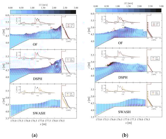
Figure 16.
Figure 15 continued: (a) time instant 6; (b) time instant 8.
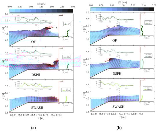
Figure 17.
Numerical comparative snapshots of the water flow on the dike. Colours are the velocity magnitude |U| according to the colour scale shown at the top of each figure. The red arrows are the velocity vectors, which are scaled for a clear visualisation. Each model snapshot has two inset graphs of Ux at the ECM location on the promenade: at the top is a time series plot of Ux in which a marker indicates the time of the snapshot, and next to the vertical wall the numerical Ux-profile is plotted over the water column at the ECM location (vertical axis is z [m]) together with the single point Ux measurement by the ECM (+marker). Adapted from the work in [3], with permission from the authors, 2020. (a) Time instant 2; (b) time instant 7.
The first main impact was identified by Gruwez et al. [3] to be caused by a plunging breaking bore pattern impacting on the vertical wall. The overturning wave arose when a large incoming bore collided with a smaller bore that was reflected against the vertical wall only a few moments before. This collision occurred at different locations on the promenade for each model and explains the timing mismatch of the Fx impact peak with EXP (see Fx graph insets in Figure 15c). The timing of the smaller bore impact corresponds with EXP in case of OF and SW8L, but is late for DSPH (time instant 1, Figure 15a). For all numerical models, the large incoming bore arrived later than was observed in EXP. This means that the collision between the reflected small bore and incoming large bore was timed differently for each model, with repercussions for the subsequent impact of the overturned wave on the vertical wall.
The best result is obtained by the OF model, which modelled a correct timing of the smaller bore reflection against the wall, but the late arrival of the larger incoming bore (i.e., by approximately 0.3 s) caused the collision to occur further from the wall than in the EXP (time instant 2, Figure 17a). Nevertheless, for the impact on the wall (time instants 3 and 4, Figure 15b,c), OF is able to—albeit mostly qualitatively—reproduce the shape of the pressure distribution which is distinctly different from a hydrostatic pressure distribution: both the pressure peak at PS10 for time instant 3 and the general shape of the pressure distribution at time instant 4 are captured by the model. We direct interested readers to the work in [3] for a more detailed description of this comparison. DSPH has a very similar result, but the timing of the smaller bore was late as well (i.e., by approximately 0.7 s), meaning that the collision with the larger bore occurred closer to the wall than observed in EXP (time instant 3, Figure 15b). Although the model did not capture the pressure peak at PS10 for time instant 3, it did manage to approach the pressure distribution qualitatively as well during the dynamic impact (time instant 4, Figure 15c). Although SW8L managed to get the timing of the smaller bore impact right (time instant 1, Figure 15a), the larger bore impacted the wall much later than in EXP (i.e., by approximately 1.2 s). This means that no interaction between the bores was modelled on the promenade. In any case, SWASH is a depth-integrated model, so it is inherently not able to model overturning waves explicitly. Moreover, only hydrostatic pressure distributions are provided by the model to avoid spurious numerical oscillations (Section 2.3). However, even with those limitations, SW8L (and SW1L) still managed to predict an Fx peak during the dynamic impact (time instant 4, Figure 15c), but the pressure distribution remains hydrostatic and therefore no local pressure peaks were captured at all.
After the dynamic impact (time instant 4), the bore ran up the vertical wall (time instant 5, Figure 15d) and reflected, causing a second quasi-static Fx peak (time instant 6, Figure 16a). In both the OF and DSPH results, a clockwise vortex formed near the bottom of the wall during the run-up process. However, in case of DSPH, this vortex was much stronger and lasted during the quasi-static Fx peak as well. The p distribution of EXP was mostly hydrostatic, except for a small local peak at PS06 (time instant 5), which seems to have been captured qualitatively by DSPH. On the other hand, the strong vortex modelled by DSPH also caused a non-hydrostatic p distribution during time instant 6, while it was mostly hydrostatic in EXP. In this time instant, again OF was closest to the EXP observation. SW8L was not successful in correctly predicting the wave run-up against the vertical wall during reflection of the large impacting bore (time instant 5) and consequently underestimated p and Fx more than the other numerical models for time instants 5 and 6. During return flow (time instant 8, Figure 16b) the pressure distribution was mostly hydrostatic, and all numerical models were able to predict the p distribution well. Only DSPH shows a pressure decrease near the bottom of the wall (PS01), possibly caused by the persistent vortex modelled there, but now further removed from the wall compared to the previous time instants 5 and 6.
In terms of U, generally similar velocity field patterns are found for all three numerical models with differences mostly explained by (small) phase differences of the individual bores interacting on the promenade or limitations in the physics it can represent (in case of SWASH). Considering the velocity profile at the ECM location during a maximum incident Ux event (time instant 2, Figure 15b) followed by a maximum return flow Ux event (time instant 7, Figure 17b), it can be seen that all numerical models underestimate Ux of EXP close to the bottom for the incident bore (time instant 2), while OF predicts it very well, DSPH slightly underestimates it, and SW8L overestimates it during the return flow (time instant 7).
3.6. Computational Cost
Not only the model performance is of importance in practical applications of numerical models, but also the computational cost that it requires. An overview is provided in Table 6 of the model resolution, total amount of grid cells/particles and corresponding computational cost for the computational hardware applied. The numerical convergence analyses in Appendix A showed that the main characteristics of η at the toe of the dike would not change more than 5% by increasing the grid or initial particle distance resolution beyond the values provided in Table 6. For OF, this was achieved by Δx = Δz = H/20 = Lm,t/260 (with H the wave height and Lm,t the mean wave length of the SW components at the dike toe), for DSPH by dp = H/50 = Lm,t/585 and for SWASH by Δx = Lm,o/170 = Lm,t/60 (with Lm,o the mean wave length of the SW components offshore).
Table 6.
Grid resolution, number of cells and approximate computational times of each applied numerical model.
Because of its Lagrangian description of the NS equations, DSPH has the advantage that it can be highly parallelised and is therefore able to make use of the many computational cores available in GPUs. On the other hand, OF and SWASH can be run in a parallelised way as well, but only on CPU cores, which are typically much less numerous. Different hardware and different amounts of cores are applied for each model, so only a qualitative comparison of the computational cost is possible. However, the applied hardware is in each case currently representative of what is typically available at research labs. OF and DSPH were run on multiple cores (CPU and GPU respectively) and SWASH on a single core.
Because the flow in the vertical dimension is fully resolved by OF and DSPH in addition to the horizontal dimension and at a much higher resolution, their computational cost is significantly higher than for the depth-averaged SW1L model. The increase of calculation time compared to SW1L is about 5000 times in case of OF and 1000 times for DSPH even though DSPH has more than 4 times the computational points than the OF model grid. Adding eight vertical layers to the SWASH model (SW8L) leads to a factor 7 increase in calculation time (on a single core machine). Although it will not affect this conclusion, it should be noted, however, that the SWASH computational domain is about 25% shorter compared to OF and DSPH, because waves are generated at the WG02 location in the SWASH model (Figure 3).
In the computational cost, the model setup time should also be included. This depends on the experience of the practitioner, so the model setup time is only discussed here in general terms based on experienced practitioners for each respective model. SWASH is the most straightforward in this respect and requires the least “hands-on” time. The model setup of DSPH is also quite straightforward, where SPH particles are initially created on nodes of a regular lattice in a few seconds. The model domain boundaries and the water volume are defined by particles in DSPH, while an intricate mesh is needed for Eulerian models such as OF. Fortunately, the mesh generation for OF has been made much smoother thanks to automatic mesh generation algorithms such as cfMesh as applied here. Still, OF is found to require the most model setup time (i.e., typically more than double). This is certainly the case when a variable grid resolution is used because the refinement zones need to be defined beforehand, and this can only be done accurately by having a reliable estimation of the location of the surface elevation. This is most easily obtained from a fast SWASH model result (at least for the wave propagation until the dike toe), or alternatively by introducing refinement zones iteratively between OF model runs.
4. Discussion
4.1. Inter-Model Comparison of Wave Transformation Processes
4.1.1. Wave Transformation Processes Until the Dike Toe
The main prerequisite for a numerical model to obtain accurate results of the processes on the dike (i.e., wave overtopping [27] and bore interactions [3]) is that the wave transformation and wave setup are predicted well towards and particularly at the dike toe.
Because DSPH was the only model able to reproduce the wave paddle motion exactly as in the experiment (note: OF has the functionality, but numerical instabilities prevented its successful application [3]), it is not surprising that it was the best performing model in terms of η from offshore up to the shoaling zone (Figure 9 and Figure 11, WG02-WG07). In the EXP, Hrms decreased slightly (4%) between the offshore region (Figure 9, WG02-WG04) and the shoaling zone (WG07), indicating an energy loss greater than the Hrms gain due to shoaling, possibly due to bottom friction and/or model effects (e.g., lateral wall friction, sediment transport on the sandy slope). However, too few EXP measurement locations were available in this area to confirm this. In any case, all three applied numerical models agreed that Hrms first decreased towards the foreshore toe, and then increased due to SW shoaling (Figure 9). In case of both OF and SW1L, the Hrms decrease was more pronounced than DSPH and could be explained by wave energy losses due to bottom friction to a certain degree (i.e., in OF by the no-slip boundary and in SW1L by parameterised bottom friction). However, these energy losses cannot be explained by the bottom friction alone due to the relatively short propagation distance from the offshore model boundary to the foreshore toe of less than three wave lengths. Viscous and/or diffusive numerical schemes could have contributed as well, especially in the case of OF [45], which mostly used second order discretization schemes but also included a first order scheme (i.e., Euler time discretisation for the volume fraction of the VOF method) for numerical stability reasons [3]. Such numerical diffusion was limited as much as possible in each model by a careful selection of parameters and schemes, which is a balancing exercise between model accuracy and efficiency. DSPH is presently unable to model bottom friction and the numerical diffusion was least noticeable of all three models, causing the Hrms overestimation at WG07 by DSPH. SW1L/SW8L tended to overestimate the shoaling (mostly for the LWs) so that an overestimation similar to DSPH at WG07 was obtained. Clearly OF suffered most from (numerical) energy losses, as it started with approximately the same wave energy at the wave paddle as DSPH, but underestimated EXP at WG07. DSPH and OF did agree on the location of the mean breaking point (xb = ~120 m, Figure 9) and simulated both spilling and plunging breakers, also observed in EXP [3]. Indeed, both models previously have been shown to predict the breaking point (and hydrodynamics) similarly well for both spilling and plunging breakers (i.e., OF [69] and DSPH [12]). SW1L/SW8L, on the other hand, predicted the breaking point to be located more offshore (by about 10 m). Contrary to OF and DSPH, SWASH does not explicitly model the turbulent wave front during the breaking process, but treats it at the sub-grid level instead by assuming similarity to a hydraulic jump [25]. SW1L/SW8L therefore did not reproduce the overturning of the wave front. Moreover, the vertical resolution (or K) for both SW1L and SW8L was too low to be able to model wave breaking without the use of the HFA, which has been shown before to cause the breaking point to be predicted too much offshore in case of plunging breakers (see their Figure 5 in [25]). Based on these observations, the breakpoint was most likely better predicted by OF and DSPH than by SW1L/SW8L. Although, it should be noted that SWASH has the potential to match the breakpoint location in Hrms by increasing K to 20 layers [25] (not tested). In the surf zone, DSPH and SW1L/SW8L predicted very similar wave heights until the dike toe and both models ended up slightly overestimating Hrms,EXP at the dike toe, SW1L more than DSPH (σ* in Table 2). The evolution of Hrms was also very similar for OF, but the values were lower because Hrms at the breakpoint was lower as well, with OF the only model that underestimated Hrms,EXP at the dike toe.
Both wave set-down and set-up were overestimated by DSPH compared to EXP. This overestimation in the shoaling and the surf zone was mostly caused by the overestimation of the wave height and therefore radiation stresses in the same areas. The overestimation of the offshore wave set-down (Figure 9, WG02–04) was a result of the overestimation of the wave setup in the surf zone, and because of mass conservation and a finite water mass available in the computational domain. Over about the final 5 m towards the dike toe, the wave setup suddenly increased, causing locally an even higher overestimation of the wave setup and the worst correspondence there with EXP of all three numerical models. This is most likely related to the small water depth this area relative to the particle size dp. Indeed, a similar increase in wave setup was noted by Lowe et al. [12] in the shallowest water depths near the shoreline and exacerbated for increasing dp values (see their Figure S1b of [12] in their supplementary material). The mismatch of the mean water level between OF and EXP was already explained by Gruwez el al. [3] to be a result of the static wave boundary condition treatments and the general underestimation of the wave height. At each measurement location, the wave set-down/up was best predicted by the SW1L model.
The accuracy of the wave phases was best for DSPH and approximately equal for OF and SW1L in the offshore zone (Figure 11, WG02–WG04). However, in the surf zone towards the dike toe, DSPH had the most wave phase errors (Figure 11, WG13–WG14), mostly caused by both the SWs (Figure 4d,e) and LWs (Figure 5c,d) lagging behind those of EXP. In case of SW1L/SW8L, the wave phase accuracy decreased at WG07 (Figure 11), where the SWs were leading those of EXP near its predicted breaking point (Figure 4b). This trend mostly continued in the surf zone until the dike toe (Figure 4d,e), where SW1L/SW8L obtained a slightly better phase accuracy than DSPH (Figure 11 and R in Table 2). The simplified wave breaking modelling with the HFA is thought to be the main cause for the increased phase errors of the ηsw result in the surf zone observed for SW1L in Figure 11.
The observed numerical model accuracy for the reproduction of the wave amplitude, wave set-up and wave phase of the EXP at the dike toe, lead to OF having the highest model performance at the dike toe, followed by SW1L and DSPH (dr in Table 2). Although DSPH achieved the best wave amplitude result, the errors in both wave setup and wave phase caused it to have the lowest model performance at the dike toe location. OF also achieved the best overall model skill in terms of η over the foreshore (and promenade), with the mean skill circle having the smallest radius in the target diagram (Figure 14, left), again, respectively, followed by SW1L and DSPH.
It should be noted, however, that the results of all three models remain very close to each other right up until the dike toe, which is reflected in the model performance rating for η: at the dike toe it was Very Good for both OF and SW1L, while it was Good for DSPH, but only because the d’r value fell just below the limit for a Very Good rating (i.e., d’r,WG14,DSPH = 0.79 < 0.80, Table 2 and Table A1). This means that all three numerical models are shown to be able to represent frequency dispersion, and the nonlinear wave transformation processes: SW shoaling (Figure 4b), breaking (Figure 4c,d) and energy transfer to the subharmonic bound LW (Figure 4b–d). This is a confirmation of what has been proven before by Torres-Freyermuth et al. [70,71] for RANS modelling, by Lowe et al. [12] for DualSPHysics and Rijnsdorp et al. [26] for SWASH.
4.1.2. Bore Interactions on the Promenade and Impacts on the Vertical Wall
The numerical model performances obtained for η at the dike toe were maintained along the promenade, except for DSPH which showed an improved model performance to match with SW1L closer to the vertical wall (Figure 12). Because of SW breaking over the foreshore, transfer of energy to the LW, LW shoaling and reflection against the steep slope of the dike, the LW wave height became almost twice the SW wave height at the dike toe location (Figure 9, WG14). Indeed, Van Gent et al. [72] and Hofland et al. [73] have shown that the wave energy is dominated by LWs at the toe of a dike with a very or extremely shallow foreshore. Therefore, the LWs at the dike toe had a dominant effect on the wave overtopping processes on the dike [3], which is a confirmation of the same observation made by Lashley et al. [39]. During each crest of the LWs at the dike toe, the freeboard decreased significantly and the broken or breaking SWs were able to overtop the dike crest much more easily. Consequently, the bore interactions on the promenade depended mostly on the SWs instead. This is shown by the fact that the model performance of DSPH for ηLW at the dike toe was lower than SW1L (Figure 10), while it was higher than SW1L for ηSW at the same location, and the model performance for the total η increased on the promenade for DSPH relative to SW1L (Figure 12). This was mostly because of a better wave amplitude and phase accuracy by DSPH than SW1L/SW8L on the promenade (Table 3, σ* and R, respectively). Moreover, in terms of Ux for the bore interactions on the promenade, DSPH had a higher model performance than SW1L and was comparable to OF. In any case, the highest model performance for both η and Ux on the promenade was achieved by OF. This is mostly indicated by a higher phase accuracy than both DSPH and SW1L/SW8L and a higher amplitude accuracy than SW1L/SW8L (Table 3, R and σ*, respectively). OF obtained the highest phase accuracy on the promenade as a result of the highest wave phase accuracy achieved at the dike toe (Figure 11, WG14), especially because of the SW phase accuracy (i.e., Rsw) at the dike toe which was notably higher for OF than both DSPH and SW1L/SW8L. At the dike toe, DSPH had the highest error in by overestimating it (Table 2, B* = 0.21) more than OF and SW1L/SW8L. Nevertheless, on the promenade DSPH underestimated with a very similar result as OF and SW1L (Table 3, = −0.04). A possible cause for this change in behaviour is that thin layered flows with a water depth on the promenade were not captured by DSPH because the water depth was smaller than a couple of particles high. The fact that SW1L/SW8L was also able to achieve a Very Good model performance for the overtopped flow layer thickness on the promenade (Table 3) indicates that a very good wave overtopping accuracy has been demonstrated as well, which is a confirmation of previous validation works on wave overtopping over a dike with a shallow foreshore modelled with SWASH [27,28].
Therefore, what seems to matter the most for the accuracy of the processes on the dike is to obtain a good model performance at the toe of the dike. A correct wave phase and wave setup at the dike toe is more important for a correct wave impact simulation than a correct wave amplitude at the dike toe. Indeed, OF had the best overall performance at the dike toe, with the best wave phase and close second best wave setup prediction (Table 2), while underestimating the wave amplitude, and showed the best model performance in terms of η and Ux on the promenade (Table 3), and consequently also for Fx and p at the vertical wall (Table 4, Figure 13 and Figure 14b). Conversely, DSPH had the best wave amplitude, but the worst wave setup and phase prediction at the dike toe and showed a lower performance in terms of Fx at the vertical wall. In addition, the snapshot comparison of the first series of impacts at the vertical wall (Section 3.5) confirmed that the wave phase accuracy was critical to obtain the correct bore interaction pattern on top of the promenade, which was—in its turn—shown to be vital to the accuracy of the impact itself. Likewise, SW1L showed similar SW phase errors at the dike toe (Figure 11, Rsw), which consequently caused phase errors in the overtopped bores (R for SW1L/SW8L is mostly lower than OF and DSPH for both η and Ux in Table 3) and their impacts on the vertical wall (R for SW1L/SW8L is mostly lower than OF and DSPH for both p and Fx in Table 4). In Section 3.5, this manifested itself in the SW8L result by a clear phase difference in the Ux time series (Figure 17) and in the Fx time series of the main impact (Figure 15c), which were both a result of a phase error in η for the largest bore of the first wave group arriving at the dike toe (see t ~55 s in Figure 4d).
In the context of the design of vertical walls on top of the dike (e.g., storm walls and buildings), the accurate prediction of the force peak per impact event Fx,max and the total horizontal force impulse I is of particular interest. The model performance for Fx,max was found to be similar for all three applied numerical models (Table 4, dr,Fx,max). However, for I* important differences were noted, with the best total impulse prediction obtained by OF, followed by DSPH and SW1L/SW8L, respectively. For SWASH, the best result was obtained by the depth-averaged model SW1L. Adding vertical resolution (i.e., SW8L) generally improved the model performance for η along the wave flume (not shown, except at the dike toe in Table 2) and η and Ux along the promenade (Table 3). However, SW8L unexpectedly decreased the model performance for Fx compared to SW1L, with slightly worse performance for Fx,max and a higher error in I* (Table 4). The cause for this is unclear, but this might indicate that SW1L’s good estimation of Fx could be—in part—caused by chance due to numerical errors (e.g., overestimation of the wave height at the toe of the dike, Table 2, σ* > 1.00). Nevertheless, the SW1L/SW8L model results show that SWASH can provide similar or only slightly worse model performance for Fx compared to OF and DSPH, including the best estimation of Fx,max per impact event, albeit with an important underestimation of I.
This comparison shows that SWASH, with a hydrostatic assumption for the calculation of Fx, is able to provide a similarly accurate prediction of Fx (especially Fx,max) compared to more complex and computationally expensive RANS or SPH models. Xie and Chu [19] already showed that with the hydrostatic pressure assumption, a tsunami bore impact force on a vertical wall can be obtained similar to OF (which includes non-hydrostatic effects as well) and experimental data. This is confirmed and extended here for overtopped bore impacts on dike-mounted vertical walls, determined from the SW1L/SW8L results based on the hydrostatic pressure only. Still, SW1L/SW8L had a lower model performance than OF and DSPH for Fx, most probably due to the hydrostatic pressure assumption. Indeed, while Whittaker et al. [23] found that the perturbed hydrostatic pressure gives an accurate approximation to the pulsating horizontal force on a gently sloped seawall, they expected the hydrodynamic contributions in Fx to increase in importance for steeper slopes (including vertical walls), particularly in the case of breaking waves. In addition, it is important to note that a low-pass filter was applied to both the experimental and numerical p and Fx time series that mostly removed high frequency oscillations in the dynamic impact peak of the double peaked signal caused by a bore impact (Section 2.3). Because these oscillations are stochastic by nature, not even REXP was able to reproduce them exactly and they cannot be reproduced by deterministic numerical models (which is why they were filtered out). However, in both the OF and DSPH results such high-frequency oscillations were present in the unfiltered signals (not shown). Although it is unclear whether they are caused by numerical errors or actual physical processes (or a combination thereof), it still might suggest that they are able to represent this phenomenon in some capacity. Conversely, in the case of SW1L/SW8L, even in the unfiltered Fx signal no such high-frequency oscillations were observed, because of the hydrostatic assumption.
Finally, OF is the only numerical model considered here that simulated both the water and air phases, albeit as incompressible and immiscible fluids. Although OF had the best overall model performance and some influence of the air was noted (especially for plunging wave impacts on the vertical wall), no immediate proof has been found that the air phase contributed positively to the model performance for the parameters considered in this paper. It is estimated that if there would have been a contribution (positive or otherwise), the effect would be small compared to the relatively larger errors in wave setup, height and phase. The fact that OF includes the air phase was actually more cumbersome to the simulation than an advantage. Indeed, spurious velocities in the air phase near the water–air interface caused significantly reduced time steps and consequently a large increase in computational cost [45,46]. Although, as discussed by Gruwez et al. [3], these spurious velocities can be overcome thanks to recent developments in OpenFOAM® [74] (however, presently not available open source).
4.2. Application Feasibility of the Numerical Models for a Design Case
This section provides recommendations on which of the three numerical models to use when, during the design of a structure on a dike with a shallow foreshore, a numerical model is used as an alternative to or complementary to experimental modelling in a wave flume. In such a case, typically a maximum expected wave impact force Fmax and corresponding impulse I for given design conditions has to be predicted. Generally, two methods can be used to achieve this:
- Modelling of a short-duration focused wave group. This method has been developed recently [23,75] based on the NewWave approach [76] and aims to reproduce the extreme event that causes Fmax in an irregular wave train, thereby significantly reducing the test duration.
- Modelling of an irregular wave train of sufficiently long duration (i.e., 1000 waves or more) to obtain statistically relevant results for Fmax.
In this paper, bichromatic waves were used for the inter-model comparisons, which included many of the wave transformation processes found in irregular waves and focused wave groups (e.g., frequency dispersion, and transfer of wave energy to sub- and superharmonics), so that this case still provides a good indication of how each numerical model would perform in terms of accuracy in each of these design methods.
Disregarding for a moment the numerical model performances for the estimation of Fmax (more on that later), the computational time necessary to achieve a result becomes the determinative factor in the choice between the three considered models. In the first method, a single wave group is modelled to obtain a certain focus location relative to the structure. Such a test duration has a similar length to the test considered here. For this design approach a standalone application of all three considered numerical models is therefore possible. However, many combinations of the focus location and phase at focus might be necessary to obtain the “true” Fmax for a given offshore design wave state [23], which would be more challenging (in terms of runtime) for standalone application of especially OF, but also DSPH.
In the second method, an irregular wave train typically needs to be modelled for a much longer duration (i.e., 1000 waves or about a 55 times longer duration than the test considered here). The high computational time or resources that this currently would require, proves unpractical for both OF and DSPH (i.e., in terms of time: approximately 190 days and 35 days, respectively, based on Table 6), especially in case of coastal structures with a shallow foreshore where the lengthy foreshore needs to be included in the computational domain. Moreover, in case of DSPH an increase in errors in the η results was noted in the surf zone compared to EXP towards the end of the simulation (i.e., for t > 120 s in Figure 4c–e and Figure 5c,d). For longer simulations it is possible that this accumulation of errors continues and exacerbates. A smaller particle size might solve this, but would increase the calculation time significantly. Therefore, similar to OF, DSPH would benefit from (adaptive) mesh refinement or variable resolution [77] to reduce the computational cost and increase the accuracy near and on top of the dike. Alternatively, coupling or hybridization with a computationally less demanding but accurate model regarding the wave transformations over the foreshore until the dike toe (e.g., SWASH [27]) is a possibility as well. Such a coupling would dramatically reduce the required computational time necessary to model this type of cross section, making longer simulations of 1000 irregular waves a practical possibility. For DSPH, such a hybridization with SWASH is already available [78]. Work in this direction for OF has been initiated by Vandebeek et al. [79,80]. The authors actively encourage further development and validation of these coupling approaches, especially since the coupling zone in current developments is located in the pre-breaking area, so that still a large area of the foreshore needs to be included in the model domain of DSPH and OF. Challenges remain in moving the coupling zone more towards the dike toe location, which would achieve the highest reduction in computational cost without losing too much accuracy for the processes on the dike. As opposed to both OF and DSPH, standalone application of SWASH for this method is definitely practically feasible for both a single layer and multi-layer approach, at least purely from a computational cost standpoint (i.e., for SW1L and SW8L approximately 1 h and 6 h, respectively, for an irregular wave train of 1000 waves, based on Table 6, and with even faster calculation times for parallel runs).
Another consideration in the choice between the three considered numerical models is of course the accuracy of the numerical model in the estimation of Fx itself. In terms of I, SWASH clearly underperformed compared to both DSPH and OF. Therefore, when I is important, OF is the recommended model to apply (i.e., highest value for I*, Table 4). However, the inter-model comparison provided in this paper has shown that all three models have a similar model performance in terms of estimation of Fx,max for individual impact events (Table 4, dr,Fx,max). This means that for the estimation of Fx,max, SWASH is actually the most recommended model to apply, because of the lowest computational cost. Although, it is important to note that this conclusion is only valid for a relatively straightforward geometry of a dike slope, promenade and vertical wall. For more complex geometries of dikes (e.g., presence of roughness elements, small storm walls with or without parapets, etc.), all numerical models considered in this paper remain untested and especially the simplified model SWASH is expected to be insufficiently accurate, because the importance of vertical flows would increase. However, a meshless approach could potentially be the most capable to capture nonlinearities of fluid–structure interactions derived from extremely complex dike geometries.
Finally, the snapshot comparisons in Section 3.5 have shown that the p distributions modelled by OF resembled most closely to EXP during each stage of a bore impact on the vertical wall and is therefore recommended when pressure distributions are of particular interest. It is estimated that DSPH should be capable of the same when the bore interactions are modelled more correctly by lowering the wave phase error. On the other hand, because the non-hydrostatic effects in p needed to be disregarded due to numerical discrepancies, SW1L/SW8L is limited to hydrostatic p distributions.
5. Conclusions
Three open source CFD models were applied in 2DV to reproduce large-scale wave flume experiments of bichromatic wave transformations over a cross section of a hybrid beach-dike coastal defence system, consisting of a steep-sloped dike with a mildly-sloped and very shallow foreshore, and finally wave impact on a vertical wall: (i) the RANS solver interFoam of OpenFOAM® (OF), (ii) the weakly compressible SPH model DualSPHysics (DSPH) and (iii) the non-hydrostatic NLSW equations model SWASH (depth-averaged (K = 1): SW1L, and multi-layered (K = 8): SW8L). The inter-model comparison of those three numerical models to the experiment (EXP) demonstrated that they are all capable of modelling the dominant wave transformation (i.e., propagation, shoaling, wave breaking, energy transfer from the SW components to the bound LW via nonlinear wave–wave interactions) and the wave–structure interaction (i.e., individual wave overtopping, bore interactions, and reflection processes) processes involved leading up to the impacts on the vertical wall, albeit with a varying degree of accuracy. Based on a time series comparison, all three applied numerical models initially appeared to have a good correspondence of η, Ux, p and Fx to EXP. However, consistent differences between the models were hard to distinguish in this purely qualitative way. The accuracy was subsequently quantified more objectively by employing model performance statistics and the nature of the errors was exposed by pattern statistics. These statistics were plotted over the wave flume to provide spatial insight into the model performance, and the pattern statistics were plotted in a skill diagram, which visualised both the model performance and pattern statistics in a summarised way. In all statistics, the original EXP was used as the comparison reference, so that the repeated experiment (REXP) statistics could be used as reference for an ideal numerical model performance. While none of the numerical models managed to achieve such an ideal model performance, a rating of Good to Very Good was achieved by all three of them for most parameters and measured locations. The best overall model performance was achieved by OF, but required the highest computational cost. Although DPSH managed the best reproduction of the wave height until the dike toe, accumulation of errors in the wave setup and wave phase in the surf zone and near the dike toe caused a lower model performance than OF at the dike toe and for the processes on the dike. From this, it followed that accurate modelling of the wave setup and wave phases at the dike toe seem to be most important for accurate modelling of the bore interactions on the promenade. An analysis and comparison of snapshots of the numerical results on the dike revealed that these bore interactions are determinative for the impacts on the vertical wall. Even though SWASH is a much more simplified model than both OF and DSPH, it is shown to provide very similar results for the wave transformations until the dike toe and even for the processes on the dike and impacts on the vertical wall. When the impulse of the force on the structure is of lesser importance, SWASH is even most recommended for this application, because it is able to predict Fx,max relatively accurate for each individual impact, with a significantly reduced computational cost, compared to OF and DSPH. However, SWASH is limited to hydrostatic pressure profiles for the impacts on the vertical wall, which is not always valid during more dynamic impact events. In addition, when the force impulse is of importance and more accurate and detailed wave–dike interactions are needed, OF is most recommended for this application. For future work, it is suggested to investigate whether the same conclusion is valid (particularly regarding applicability of SWASH) in the case of more complex dike geometries.
Author Contributions
Conceptualization, V.G., C.A., T.S., and P.T.; methodology, V.G.; validation, V.G. and M.S.; formal analysis, V.G.; investigation, V.G., C.A., T.S., M.S., and L.C.; resources, P.T.; data curation, V.G., M.S. and L.C.; writing—original draft preparation, V.G.; writing—review and editing, V.G., C.A., T.S., M.S., L.C., A.K., and P.T.; visualization, V.G. and M.S.; supervision, P.T. and A.K.; project administration, P.T.; funding acquisition, P.T. and A.K. All authors have read and agreed to the published version of the manuscript.
Funding
This research was part of the CREST (Climate REsilient CoaST) project (http://www.crestproject.be/en), funded by the Flemish Agency for Innovation by Science and Technology, grant number 150028. The work described in this section was supported by the European Community′s Horizon 2020 Research and Innovation Programme through the grant to HYDRALABPLUS, Contract no. 654110. C.A. acknowledges funding from the European Union’s Horizon 2020 research and innovation programme under the Marie Sklodowska-Curie, grant number 792370.
Conflicts of Interest
The authors declare no conflict of interest. The funders had no role in the design of the study; in the collection, analyses, or interpretation of data; in the writing of the manuscript; or in the decision to publish the results.
Appendix A. Numerical Convergence Analyses
The numerical model convergence analyses of the DSPH and SW1L/SW8L models was done following the same methodology as described by Gruwez et al. [3] for the OF model (see their Appendix A).
Appendix A.1. Model Convergence Statistics
For the convergence analysis, the four statistical error indicators as determined by [3] are considered:
- Freeboard normalised bias (NB):
- Residual error of the normalised standard deviation (RNSD):
- Residual error of the correlation coefficient (RCC):
- Normalised mean absolute error (NMAE) given by
For their interpretation, reference is made to the work in [3].
Appendix A.2. Convergence Analyses
Appendix A.2.1. DSPH
Rota Roselli et al. [59] identified the most important parameters that influence the model accuracy in terms of nonlinear wave propagation, among them the smoothing length hSPH, the artificial viscosity parameter αav and the initial particle distance dp. However, the current case also includes wave transformations over a beach with decreasing water depth towards the dike, for which dp is found to be the most important parameter. The convergence analysis for DSPH is therefore focused on dp (Figure A1).

Figure A1.
DSPH model inter-particle distance dp convergence analysis of the η time series at the WG locations along the flume up to the dike toe (WG14), based on (a) the normalised bias, (b) the residual normalised standard deviation, (c) the residual correlation coefficient, and (d) the normalised mean-absolute-error. The reference is the highest resolution simulation with dp = 0.02 m.
Three initial particle distances (i.e., dp = 0.04 m, 0.03 m, 0.024 m) are compared to the finest resolution (i.e., dp = 0.02 m). In Figure A1 it is shown that for dp = 0.024 m, most statistical errors stay close to 5% at the toe of the dike, but approaches 8% for the NB, which is too high to be able to assume a converged state. This indicates that the resolution might still be too low to be able to sufficiently resolve the wave setup at the toe of the dike (~0.05 m based on the experimental result). To check convergence of NB an even higher resolution of dp = 0.01 m would be needed. However, this resolution was not practically feasible due to the huge amounts of data and computational costs involved. Therefore, the initial inter-particle distance dp of 0.02 m is assumed to be a sufficiently converged resolution and is used for the analysis in the paper.
Appendix A.2.2. SWASH
In case of the SWASH model, the convergence analysis is focused on the grid resolution. Grid cell sizes Δx = 0.2, 0.4 and 0.8 m are considered, and the convergence statistics are applied with reference to the finest resolution (Δx = 0.1 m). The result in Figure A2 shows that the convergence errors of Δx = 0.2 m stay within +/−5% of the finest resolution. A resolution of Δx = 0.2 m is therefore used for the analysis in the paper. The same conclusion is valid for both SW1L and SW8L (not shown).

Appendix B. Numerical Model Performance and Pattern Statistics
In this appendix, the equations are provided of the numerical model performance and pattern statistics used in this paper. For more descriptions and interpretations, reference is made to the work in [3]. The general numerical model performance is evaluated by applying Willmott’s refined index of agreement dr [81]:
where dr is bounded by [−1.0, 1.0], c is a scaling factor and is taken equal to 2, MAE is the mean absolute error defined by
with N the number of samples in the time series, and P the predicted time series together with the pair-wise-matched observed time series O (for i = 1, 2, …, n), and MAD is the mean absolute deviation:
where the overbar represents the mean of the time series.
In addition, a relative refined index of agreement d’r was defined by [3] which provides the performance of the numerical model relative to the experimental model uncertainty (in case a repetition of the experiment is available):
where the subscripts num and rexp indicate that the statistic is evaluated respectively for the numerical and repeated experimental data, and c is again taken equal to 2. When the numerator MAEnum − MAErexp is negative (i.e., <0), the numerical error compared to the experiment is smaller than the experimental uncertainty, which means that the numerical model performance cannot be improved. In that case MAEnum − MAErexp = 0 is forced, so that d’r = 1. A classification of d’r and corresponding rating terminology as proposed by the authors of [3] is provided in Table A1.
Table A1.
Proposed classification of the relative refined index of agreement d’r and corresponding rating. Reproduced from [3], with permission from the authors, 2020.
Table A1.
Proposed classification of the relative refined index of agreement d’r and corresponding rating. Reproduced from [3], with permission from the authors, 2020.
| d’r Classification [-] | Rating |
|---|---|
| 0.90–1.00 | Excellent |
| 0.80–0.90 | Very Good |
| 0.70–0.80 | Good |
| 0.50–0.70 | Reasonable/Fair |
| 0.30–0.50 | Poor |
| (−1.00)–0.30 | Bad |
The pattern statistics are provided by:
- The normalised standard deviation σ*:
- The normalised bias B*:
- The correlation coefficient R:
References
- IPCC. The Ocean and Cryosphere in a Changing Climate. In IPCC Special Report on the Ocean and Cryosphere in a Changing Climate; IPCC: Geneva, Switzerland, 2019. [Google Scholar]
- Gruwez, V.; Vandebeek, I.; Kisacik, D.; Streicher, M.; Altomare, C.; Suzuki, T.; Verwaest, T.; Kortenhaus, A.; Troch, P. 2D overtopping and impact experiments in shallow foreshore conditions. In Proceedings of the 36th Conference on Coastal Engineering, Baltimore, MD, USA, 30 July–3 August 2018; pp. 1–13. [Google Scholar]
- Gruwez, V.; Altomare, C.; Suzuki, T.; Streicher, M.; Cappietti, L.; Kortenhaus, A.; Troch, P. Validation of RANS modelling for wave interactions with sea dikes on shallow foreshores using a large-scale experimental dataset. J. Mar. Sci. Eng. 2020, 8, 650. [Google Scholar] [CrossRef]
- Streicher, M.; Kortenhaus, A.; Altomare, C.; Gruwez, V.; Hofland, B.; Chen, X.; Marinov, K.; Scheres, B.; Schüttrumpf, H.; Hirt, M.; et al. WALOWA (WAve LOads on WAlls)-Large-Scale Experiments in the Delta Flume; SCACR: Santander, Spain, 2017. [Google Scholar]
- Sibilla, S. Fluid mechanics and the SPH method: Theory and applications. J. Hydraul. Res. 2013, 51, 339–340. [Google Scholar] [CrossRef]
- Oñate, E.; Celigueta, M.A.; Idelsohn, S.R.; Salazar, F.; Suárez, B. Possibilities of the particle finite element method for fluid-soil-structure interaction problems. Comput. Mech. 2011, 48, 307–318. [Google Scholar] [CrossRef]
- Gotoh, H.; Khayyer, A. On the state-of-the-art of particle methods for coastal and ocean engineering. Coast. Eng. J. 2018, 60, 79–103. [Google Scholar] [CrossRef]
- Colagrossi, A.; Landrini, M. Numerical simulation of interfacial flows by smoothed particle hydrodynamics. J. Comput. Phys. 2003, 191, 448–475. [Google Scholar] [CrossRef]
- Mokos, A.; Rogers, B.D.; Stansby, P.K. A multi-phase particle shifting algorithm for SPH simulations of violent hydrodynamics with a large number of particles. J. Hydraul. Res. 2017, 55, 143–162. [Google Scholar] [CrossRef]
- Monaghan, J.J.; Kos, A. Solitary waves on a Cretan beach. J. Waterw. Port. Coastal, Ocean. Eng. 1999, 125, 145–155. [Google Scholar] [CrossRef]
- Domínguez, J.M.; Altomare, C.; Gonzalez-Cao, J.; Lomonaco, P. Towards a more complete tool for coastal engineering: Solitary wave generation, propagation and breaking in an SPH-based model. Coast. Eng. J. 2019, 61, 15–40. [Google Scholar] [CrossRef]
- Lowe, R.J.; Buckley, M.; Altomare, C.; Rijnsdorp, D.; Yao, Y.; Suzuki, T.; Bricker, J. Numerical simulations of surf zone wave dynamics using Smoothed Particle Hydrodynamics. Ocean. Model. 2019, 144, 101481. [Google Scholar] [CrossRef]
- Subramaniam, S.P.; Scheres, B.; Schilling, M.; Liebisch, S.; Kerpen, N.B.; Schlurmann, T.; Altomare, C.; Schüttrumpf, H. Influence of convex and concave curvatures in a coastal dike line on wave run-up. Water 2019, 11, 1333. [Google Scholar] [CrossRef]
- St-Germain, P.; Nistor, I.; Townsend, R.; Shibayama, T. Smoothed-particle hydrodynamics numerical modeling of structures impacted by tsunami bores. J. Waterw. Port. Coastal, Ocean. Eng. 2014, 140, 66–81. [Google Scholar] [CrossRef]
- Didier, E.; Neves, D.R.C.V.; Martins, R.; Neves, M.G. Wave interaction with a vertical wall: SPH numerical and experimental modeling. Ocean. Eng. 2014, 88, 330–341. [Google Scholar] [CrossRef]
- Altomare, C.; Crespo, A.; Domínguez, J.M.; Gomez-Gesteira, M.; Suzuki, T.; Verwaest, T. Applicability of Smoothed Particle Hydrodynamics for estimation of sea wave impact on coastal structures. Coast. Eng. 2015, 96, 1–12. [Google Scholar] [CrossRef]
- Hérault, A.; Bilotta, G.; Dalrymple, R.A. SPH on GPU with CUDA. J. Hydraul. Res. 2010, 48, 74–79. [Google Scholar] [CrossRef]
- Crespo, A.; Dominguez, J.; Rogers, B.; Gómez-Gesteira, M.; Longshaw, S.; Canelas, R.; Vacondio, R.; Barreiro, A.; García-Feal, O. DualSPHysics: Open-source parallel CFD solver based on Smoothed Particle Hydrodynamics (SPH). Comput. Phys. Commun. 2015, 187, 204–216. [Google Scholar] [CrossRef]
- Xie, P.; Chu, V.H. The forces of tsunami waves on a vertical wall and on a structure of finite width. Coast. Eng. 2019, 149, 65–80. [Google Scholar] [CrossRef]
- Hu, K.; Mingham, C.; Causon, D. Numerical simulation of wave overtopping of coastal structures using the non-linear shallow water equations. Coast. Eng. 2000, 41, 433–465. [Google Scholar] [CrossRef]
- Shiach, J.B.; Mingham, C.G.; Ingram, D.M.; Bruce, T. The applicability of the shallow water equations for modelling violent wave overtopping. Coast. Eng. 2004, 51, 1–15. [Google Scholar] [CrossRef]
- Orszaghova, J.; Borthwick, A.G.; Taylor, P.H. From the paddle to the beach-A Boussinesq shallow water numerical wave tank based on Madsen and Sørensen’s equations. J. Comput. Phys. 2012, 231, 328–344. [Google Scholar] [CrossRef]
- Whittaker, C.; Fitzgerald, C.; Raby, A.; Taylor, P.; Borthwick, A.G.L. Extreme coastal responses using focused wave groups: Overtopping and horizontal forces exerted on an inclined seawall. Coast. Eng. 2018, 140, 292–305. [Google Scholar] [CrossRef]
- Zijlema, M.; Stelling, G.; Smit, P. SWASH: An operational public domain code for simulating wave fields and rapidly varied flows in coastal waters. Coast. Eng. 2011, 58, 992–1012. [Google Scholar] [CrossRef]
- Smit, P.; Zijlema, M.; Stelling, G. Depth-induced wave breaking in a non-hydrostatic, near-shore wave model. Coast. Eng. 2013, 76, 1–16. [Google Scholar] [CrossRef]
- Rijnsdorp, D.P.; Smit, P.B.; Zijlema, M. Non-hydrostatic modelling of infragravity waves under laboratory conditions. Coast. Eng. 2014, 85, 30–42. [Google Scholar] [CrossRef]
- Suzuki, T.; Altomare, C.; Veale, W.; Verwaest, T.; Trouw, K.; Troch, P.; Zijlema, M. Efficient and robust wave overtopping estimation for impermeable coastal structures in shallow foreshores using SWASH. Coast. Eng. 2017, 122, 108–123. [Google Scholar] [CrossRef]
- Suzuki, T.; Altomare, C.; Yasuda, T.; Verwaest, T. Characterization of overtopping waves on sea dikes with gentle and shallow foreshores. J. Mar. Sci. Eng. 2020, 8, 752. [Google Scholar] [CrossRef]
- Vanneste, D.F.; Altomare, C.; Suzuki, T.; Troch, P.; Verwaest, T. Comparison of numerical models for wave overtopping and impact on a sea wall. Coast. Eng. Proc. 2014, 1, 5. [Google Scholar] [CrossRef]
- Buckley, M.; Lowe, R.; Hansen, J. Evaluation of nearshore wave models in steep reef environments. Ocean. Dyn. 2014, 64, 847–862. [Google Scholar] [CrossRef]
- Booij, N.; Ris, R.C.; Holthuijsen, L. A third-generation wave model for coastal regions: 1. Model description and validation. J. Geophys. Res. Space Phys. 1999, 104, 7649–7666. [Google Scholar] [CrossRef]
- Roelvink, D.; Reniers, A.; Van Dongeren, A.; Vries, J.V.T.D.; McCall, R.; Lescinski, J. Modelling storm impacts on beaches, dunes and barrier islands. Coast. Eng. 2009, 56, 1133–1152. [Google Scholar] [CrossRef]
- St-Germain, P.; Nistor, I.; Readshaw, J.; Lamont, G. Numerical modeling of coastal dike overtopping using SPH and non-hydrostatic NLSW equations. In Proceedings of the 34th Conference on Coastal Engineering, Seoul, Korea, 15–20 June 2014. [Google Scholar]
- Park, H.; Do, T.; Tomiczek, T.; Cox, D.T.; Van De Lindt, J.W. Numerical modeling of non-breaking, impulsive breaking, and broken wave interaction with elevated coastal structures: Laboratory validation and inter-model comparisons. Ocean. Eng. 2018, 158, 78–98. [Google Scholar] [CrossRef]
- Higuera, P.; Lara, J.L.; Losada, I.J. Three-dimensional interaction of waves and porous coastal structures using OpenFOAM®. Part I: Formulation and validation. Coast. Eng. 2014, 83, 243–258. [Google Scholar] [CrossRef]
- Higuera, P.; Lara, J.L.; Losada, I.J. Three-dimensional interaction of waves and porous coastal structures using OpenFOAM®. Part II: Application. Coast. Eng. 2014, 83, 259–270. [Google Scholar] [CrossRef]
- IHFOAM Team. IHCantabria. Available online: https://ihfoam.ihcantabria.com/ (accessed on 5 November 2020).
- González-Cao, J.; Altomare, C.; Crespo, A.; Domínguez, J.; Gómez-Gesteira, M.; Kisacik, D. On the accuracy of DualSPHysics to assess violent collisions with coastal structures. Comput. Fluids 2019, 179, 604–612. [Google Scholar] [CrossRef]
- Lashley, C.H.; Zanuttigh, B.; Bricker, J.D.; Van Der Meer, J.; Altomare, C.; Suzuki, T.; Roeber, V.; Oosterlo, P. Benchmarking of numerical models for wave overtopping at dikes with shallow mildly sloping foreshores: Accuracy versus speed. Environ. Model. Softw. 2020, 130, 104740. [Google Scholar] [CrossRef]
- Cappietti, L.; Simonetti, I.; Esposito, A.; Streicher, M.; Kortenhaus, A.; Scheres, B.; Schuettrumpf, H.; Hirt, M.; Hofland, B.; Chen, X. Large-scale experiments of wave-overtopping loads on walls: Layer thicknesses and velocities. Ocean. Eng. 2018, 7, 28. [Google Scholar] [CrossRef]
- Kortenhaus, A.; Streicher, M.; Gruwez, V.; Altomare, C.; Hofland, B.; Chen, X.; Marinov, K.; Vanneste, D.; Willems, M.; Suzuki, T.; et al. WALOWA (WAve LOads on WAlls)-Large-scale Experiments in the Delta Flume on Overtopping Wave Loads on Vertical Walls. Zenodo 2019. [Google Scholar] [CrossRef]
- OpenFOAM Foundation. Available online: https://openfoam.org/ (accessed on 6 August 2019).
- Berberović, E.; Van Hinsberg, N.P.; Jakirlić, S.; Roisman, I.V.; Tropea, C. Drop impact onto a liquid layer of finite thickness: Dynamics of the cavity evolution. Phys. Rev. E 2009, 79, 036306. [Google Scholar] [CrossRef]
- Deshpande, S.S.; Anumolu, L.; Trujillo, M.F. Evaluating the performance of the two-phase flow solver interFoam. Comput. Sci. Discov. 2012, 5, 014016. [Google Scholar] [CrossRef]
- Larsen, B.E.; Fuhrman, D.R.; Roenby, J. Performance of interFoam on the simulation of progressive waves. Coast. Eng. J. 2019, 61, 380–400. [Google Scholar] [CrossRef]
- Roenby, J.; Larsen, B.E.; Bredmose, H.; Jasak, H. A new volume-of-fluid method in OpenFOAM. In Proceedings of the VII International Conference on Computational Methods in Marine Engineering, Gothenburg, Sweden, 13–15 May 2017. [Google Scholar]
- Higuera, P. phicau/olaFlow: CFD for Waves, Zenodo: Geneva, Switzerland, 2018. [CrossRef]
- Larsen, B.E.; Fuhrman, D.R. On the over-production of turbulence beneath surface waves in Reynolds-averaged Navier-Stokes models. J. Fluid Mech. 2018, 853, 419–460. [Google Scholar] [CrossRef]
- Larsen, B.E. stabRAS_OF50. 2018. Available online: https://github.com/BjarkeEltardLarsen/StabRAS_OF50 (accessed on 18 September 2018).
- DualSPHysics Team. DualSPHysics: GPU and OpenMP based Smoothed Particle Hydrodynamics. Available online: https://dual.sphysics.org/ (accessed on 14 August 2019).
- Wendland, H. Piecewise polynomial, positive definite and compactly supported radial functions of minimal degree. Adv. Comput. Math. 1995, 4, 389–396. [Google Scholar] [CrossRef]
- Monaghan, J.J. Smoothed particle hydrodynamics. Annu. Rev. Astron. Astrophys. 1992, 30, 543–574. [Google Scholar] [CrossRef]
- Dalrymple, R.A.; Rogers, B. Numerical modeling of water waves with the SPH method. Coast. Eng. 2006, 53, 141–147. [Google Scholar] [CrossRef]
- Molteni, D.; Colagrossi, A. A simple procedure to improve the pressure evaluation in hydrodynamic context using the SPH. Comput. Phys. Commun. 2009, 180, 861–872. [Google Scholar] [CrossRef]
- Fourtakas, G.; Dominguez, J.M.; Vacondio, R.; Rogers, B. Local uniform stencil (LUST) boundary condition for arbitrary 3-D boundaries in parallel smoothed particle hydrodynamics (SPH) models. Comput. Fluids 2019, 190, 346–361. [Google Scholar] [CrossRef]
- English, A.; Domínguez, J.M.; Vacondio, R.; Crespo, A.J.C.; Stansby, P.K.; Lind, S.J.; Gómez-Gesteira, M. Correction for dynamic boundary conditions. In Proceedings of the 14th International SPHERIC Workshop, Exeter, UK, 25–27 June 2019. [Google Scholar]
- Altomare, C.; Domínguez, J.; Crespo, A.; González-Cao, J.; Suzuki, T.; Gómez-Gesteira, M.; Troch, P. Long-crested wave generation and absorption for SPH-based DualSPHysics model. Coast. Eng. 2017, 127, 37–54. [Google Scholar] [CrossRef]
- Vacondio, R.; Altomare, C.; De Leffe, M.; Hu, X.Y.; Le Touzé, D.; Lind, S.; Marongiu, J.-C.; Marrone, S.; Rogers, B.; Souto-Iglesias, A. Grand challenges for Smoothed Particle Hydrodynamics numerical schemes. Comput. Part. Mech. 2020, 1–14. [Google Scholar] [CrossRef]
- Roselli, R.A.R.; Vernengo, G.; Altomare, C.; Brizzolara, S.; Bonfiglio, L.; Guercio, R. Ensuring numerical stability of wave propagation by tuning model parameters using genetic algorithms and response surface methods. Environ. Model. Softw. 2018, 103, 62–73. [Google Scholar] [CrossRef]
- The SWASH team. SWASH-User Manual (v4.01A); Delft University of Technology, Faculty of Civil Engineering and Geosciences, Environmental Fluid Mechanics Section: Delft, The Netherlands, 2017. [Google Scholar]
- The SWASH team. SWASH-User Manual (v5.01); Delft University of Technology, Faculty of Civil Engineering and Geosciences, Environmental Fluid Mechanics Section: Delft, The Netherlands, 2018. [Google Scholar]
- Mansard, E.P.; Funke, E.R. The measurement of incident and reflected spectra using a least squares method. Coast. Eng. Proc. 1980, 1. [Google Scholar] [CrossRef]
- Lykke Andersen, T. WaveLab. Available online: https://www.hydrosoft.civil.aau.dk/wavelab/ (accessed on 31 August 2019).
- Jacobsen, N.G.; Van Gent, M.R.A.; Capel, A.; Borsboom, M. Numerical prediction of integrated wave loads on crest walls on top of rubble mound structures. Coast. Eng. 2018, 142, 110–124. [Google Scholar] [CrossRef]
- Taylor, K.E. Summarizing multiple aspects of model performance in a single diagram. J. Geophys. Res. Space Phys. 2001, 106, 7183–7192. [Google Scholar] [CrossRef]
- Willmott, C.J.; Matsuura, K.; Robeson, S.M. Ambiguities inherent in sums-of-squares-based error statistics. Atmospheric Environ. 2009, 43, 749–752. [Google Scholar] [CrossRef]
- Jolliff, J.K.; Kindle, J.C.; Shulman, I.; Penta, B.; Friedrichs, M.A.; Helber, R.; Arnone, R.A. Summary diagrams for coupled hydrodynamic-ecosystem model skill assessment. J. Mar. Syst. 2009, 76, 64–82. [Google Scholar] [CrossRef]
- Bullock, G.; Obhrai, C.; Peregrine, D.; Bredmose, H. Violent breaking wave impacts. Part 1: Results from large-scale regular wave tests on vertical and sloping walls. Coast. Eng. 2007, 54, 602–617. [Google Scholar] [CrossRef]
- Brown, S.; Greaves, D.; Magar, V.; Conley, D. Evaluation of turbulence closure models under spilling and plunging breakers in the surf zone. Coast. Eng. 2016, 114, 177–193. [Google Scholar] [CrossRef]
- Torres-Freyermuth, A.; Losada, I.J.; Lara, J.L. Modeling of surf zone processes on a natural beach using Reynolds-Averaged Navier-Stokes equations. J. Geophys. Res. Space Phys. 2007, 112. [Google Scholar] [CrossRef]
- Torres-Freyermuth, A.; Lara, J.L.; Losada, I.J. Numerical modelling of short- and long-wave transformation on a barred beach. Coast. Eng. 2010, 57, 317–330. [Google Scholar] [CrossRef]
- Van Gent, M.R.A. Physical Model Investigations on Coastal Structures with Shallow Foreshores: 2D Model Tests on the Petten Sea-Defence; Deltares: Delft, The Netherlands, 1999. [Google Scholar]
- Hofland, B.; Chen, X.; Altomare, C.; Oosterlo, P. Prediction formula for the spectral wave period T m-1,0 on mildly sloping shallow foreshores. Coast. Eng. 2017, 123, 21–28. [Google Scholar] [CrossRef]
- Vukčević, V.; Jasak, H.; Gatin, I. Implementation of the ghost fluid method for free surface flows in polyhedral finite volume framework. Comput. Fluids 2017, 153, 1–19. [Google Scholar] [CrossRef]
- Whittaker, C.; Fitzgerald, C.; Raby, A.; Taylor, P.; Orszaghova, J.; Borthwick, A. Optimisation of focused wave group runup on a plane beach. Coast. Eng. 2017, 121, 44–55. [Google Scholar] [CrossRef]
- Tromans, P.S. A new model for the kinematics of large ocean waves-Application as a design wave. In Proceedings of the 1st International Offshore and Polar Engineering Conference, Edinburgh, UK, 11–16 August 1991; Shell Research BV: Rijswijk, The Netherlands; Volume III, pp. 64–69. [Google Scholar]
- Vacondio, R.; Rogers, B.; Stansby, P.; Mignosa, P. Variable resolution for SPH in three dimensions: Towards optimal splitting and coalescing for dynamic adaptivity. Comput. Methods Appl. Mech. Eng. 2016, 300, 442–460. [Google Scholar] [CrossRef]
- Altomare, C.; Domínguez, J.M.; Crespo, A.J.C.; Suzuki, T.; Caceres, I.; Gómez-Gesteira, M. Hybridization of the wave propagation model SWASH and the meshfree particle method SPH for real coastal applications. Coast. Eng. J. 2015, 57, 1550024-1. [Google Scholar] [CrossRef]
- Vandebeek, I.; Gruwez, V.; Altomare, C.; Suzuki, T. Towards an Efficient and Highly Accurate Coupled Numerical Modelling Approach for Wave Interactions with a Dike on a Very Shallow Foreshore; Coastlab: Santander, Spain, 2018; p. 10. [Google Scholar]
- Vandebeek, I.; Toorman, E.; Troch, P. Numerical Simulation of Wave Propagation over a Sloping Beach Using a Coupled Rans-NLSWE Model. In Proceedings of the OpenFOAM Workshop, Shangai, China, 24–29 June 2018; pp. 1–4. [Google Scholar]
- Willmott, C.J.; Robeson, S.M.; Matsuura, K. A refined index of model performance. Int. J. Clim. 2012, 32, 2088–2094. [Google Scholar] [CrossRef]
Publisher’s Note: MDPI stays neutral with regard to jurisdictional claims in published maps and institutional affiliations. |
© 2020 by the authors. Licensee MDPI, Basel, Switzerland. This article is an open access article distributed under the terms and conditions of the Creative Commons Attribution (CC BY) license (http://creativecommons.org/licenses/by/4.0/).