Performance Evaluation of Wave Input Reduction Techniques for Modeling Inter-Annual Sandbar Dynamics

 , ,
, , 

Abstract
:1. Introduction
2. Overall Approach
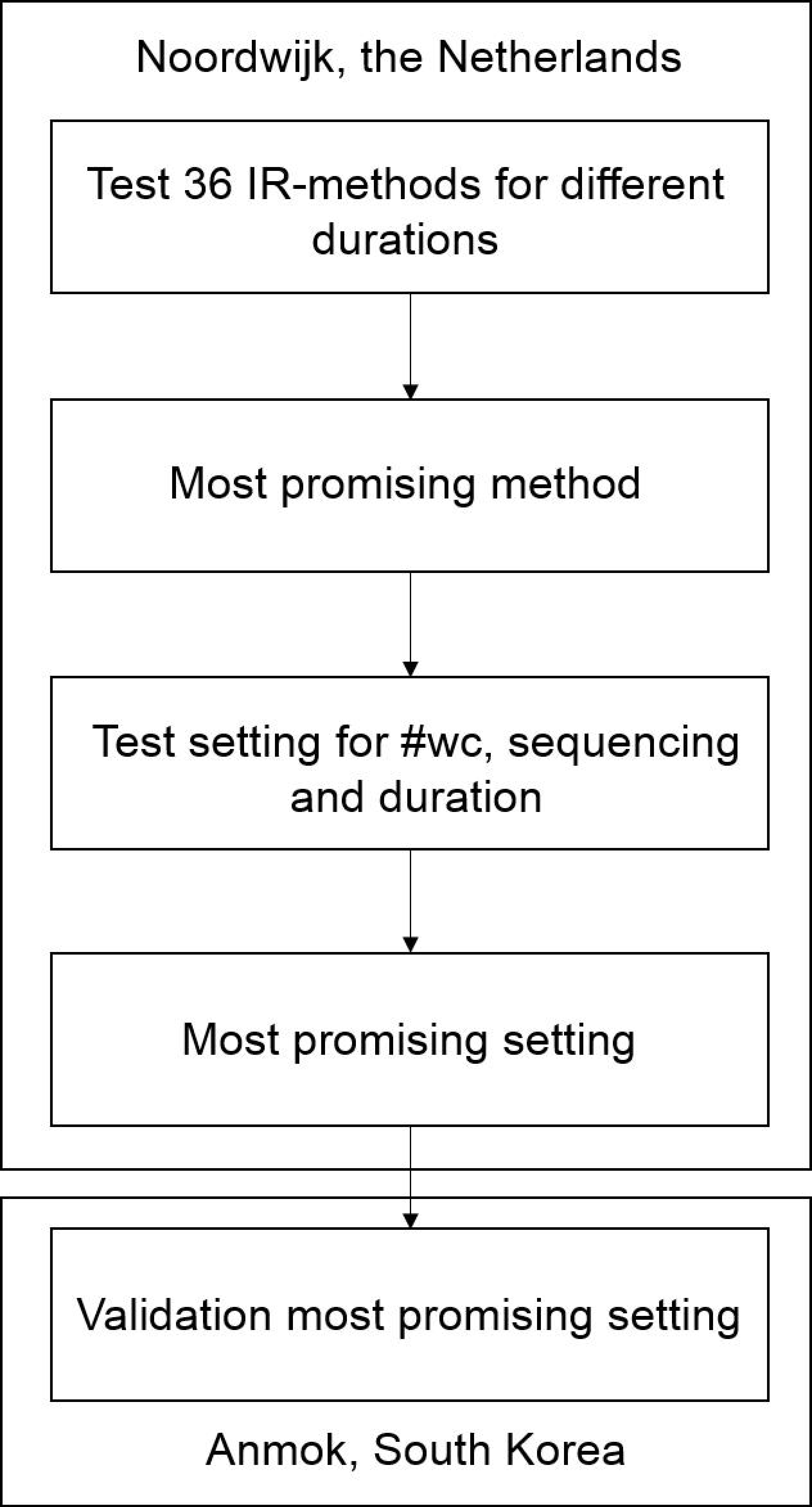
2.1. Research Steps for Testing IR-Methods and Settings
2.2. Performance Evaluation
3. Tested Input Reduction Methods
3.1. Binning Methods
3.1.1. Conditions with the Largest Transport Contribution Method
3.1.2. Fixed Bins Method
3.1.3. Energy Flux Method
3.1.4. Sediment Transport Bins Method
3.1.5. Representative Wave Approach
3.2. Clustering Methods
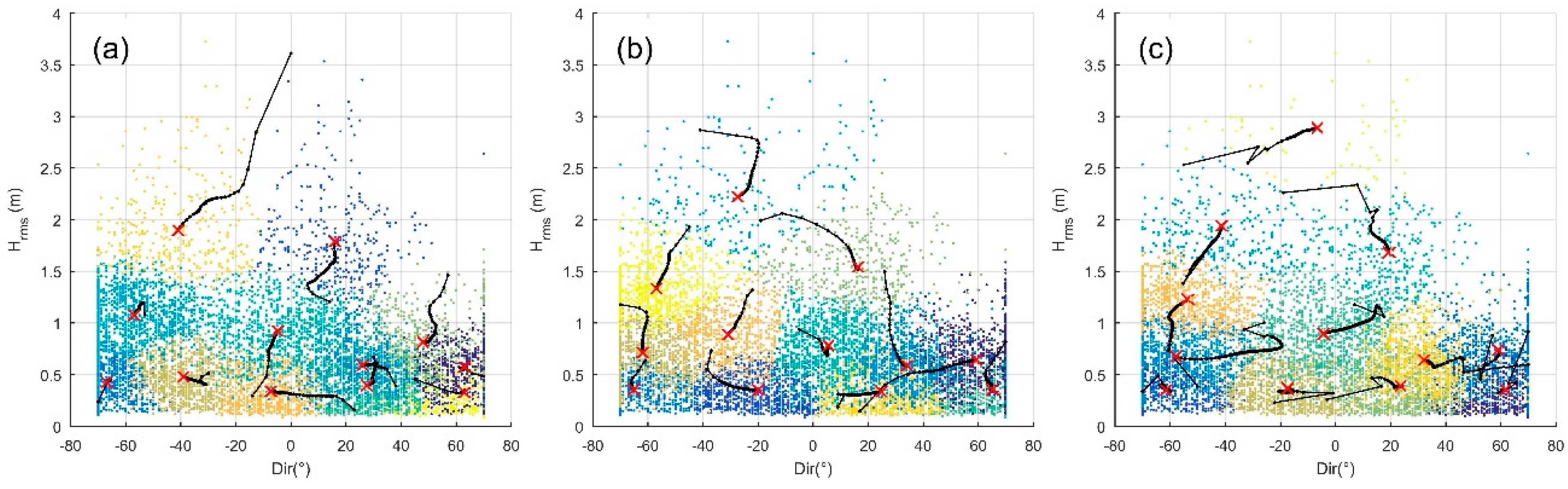
3.2.1. Maximum Dissimilarity Algorithm
3.2.2. Grouping with Equal Sediment Influence Method
3.2.3. Crisp K-Means Method
3.2.4. Fuzzy K-Means Method
3.2.5. K-Harmonic Means
4. Tested Settings
4.1. Number of Representative Wave Conditions
4.2. Sequencing Methods
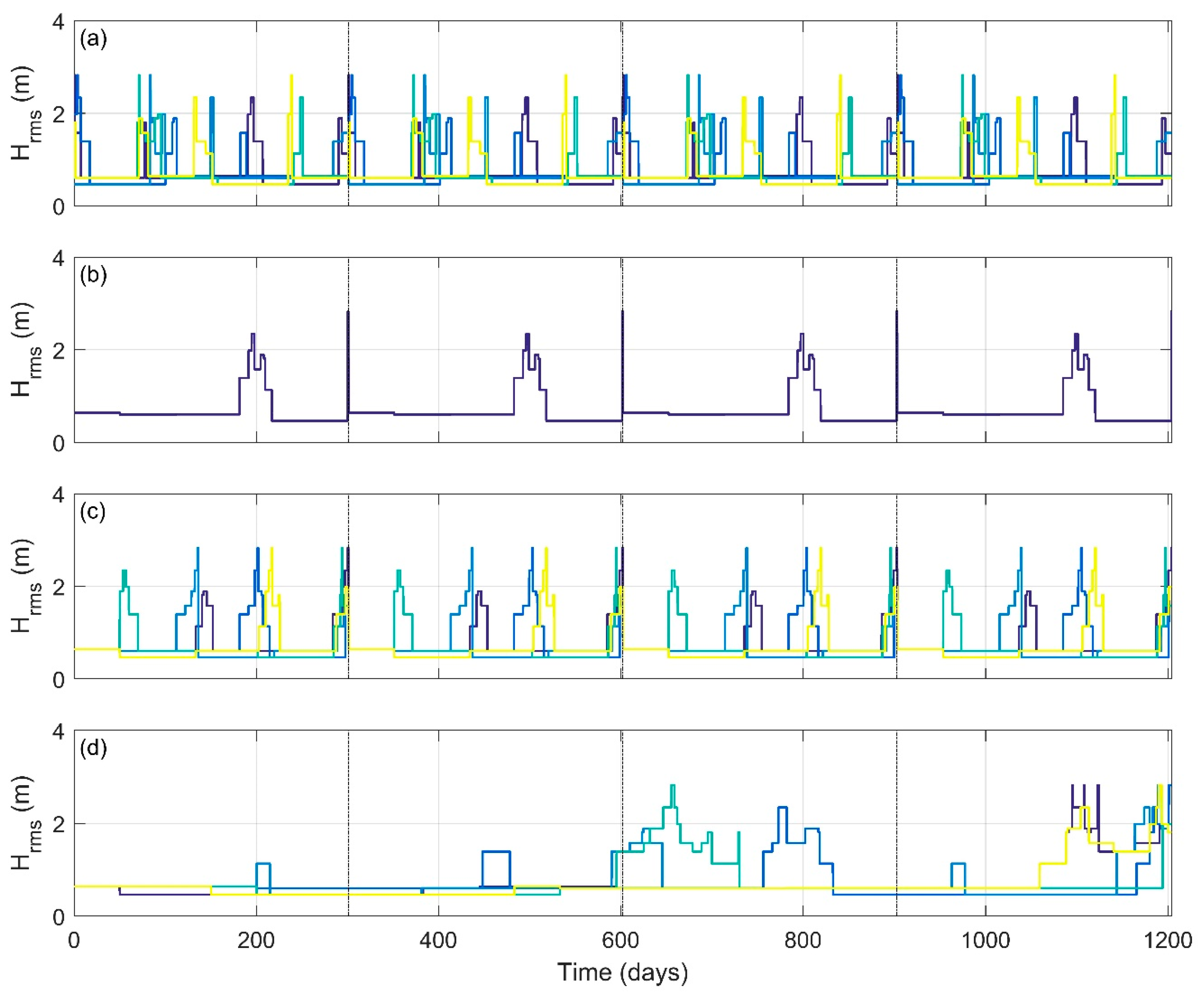
4.2.1. Random Sequencing
4.2.2. Markov Chain Sequencing
- Number the representative wave conditions stored in the database from 1 to k;
- Determine for every wave condition from the full dataset () which of the representative wave conditions in is most similar to it. In this step, a new vector is created with size N × 1 (N = number of observations of the full dataset), in which the number of the wave conditions that is most similar to each observation is stored (see Equation (8)).where is a true–false indicator that is 1 when the equation between brackets is true and 0 when it is false, is the wave observation in the full dataset, and the representative wave condition.
- Determine the Markov transitions for the wave conditions in . The Markov transitions are stored in a Markov transition matrix of size , where is the number of representative wave conditions (see Equation (9)).where is the transition probability of a representative wave condition in given a representative wave condition with transition index .
- Define two time series matrices: and . starts empty and will contain the numbers that are assigned to the wave conditions in step 1 in the sequence determined by the algorithm. contains the numbers assigned to the wave conditions in step 1 at the start of the algorithm. When a wave condition is selected by the algorithm, its number will be deleted from matrix and added to the matrix .
- Define the first wave condition () as the most similar one to the initial wave condition in the observation dataset (see Equation (10)).where and are the Euclidean distances between the initial observation of the full dataset () and a representative wave condition () and all representative wave conditions in the reduced dataset (), respectively. The number assigned to the initial wave condition () is deleted from the matrix , which reduces its size to ().
- The next wave condition to be selected for the reduced time series () is the one with the highest Markov transition probability (), conditional on the previous selected wave condition () and available in the matrix (see Equation (11)).where is a transition index and is the transition probability index of .
- Reorder the wave conditions in the database according to their assigned numbers in matrix .
4.2.3. Monte Carlo Markov Chain Sequencing
- Follow steps 1 to 2 from MC (cf. above).
- Determine the cumulative Markov transitions () for the wave conditions in . The cumulative Markov transitions are stored in a Markov transition matrix of size :
- Define two time series matrices: and as in step 4 of Section 4.2.2;
- Define the first wave condition () as the most similar one to the initial wave condition in the observation dataset as in Equation (10). The Markov transition probability of the initial wave condition () is reduced from the cumulative Markov transition matrix and the remaining cumulative probabilities are normalized. Moreover, the number assigned to the initial wave condition ()) will now be deleted from the matrix , hence, its size reduces to .
- Draw a random number between 0 and 1 (). The next wave condition to be selected () is the first occurrence with the Markov transition probability containing the random number previously defined:
- Subtract the Markov transition probability of the selected wave condition from the cumulative Markov transition matrix and normalize the remaining probabilities:
- Exclude the selected wave condition from the matrix .
- Reorder the wave conditions in the database according to their assigned numbers in matrix .
4.2.4. Monte Carlo Markov Chain with Repetition Sequencing
4.3. Wave Climate Duration
5. Results
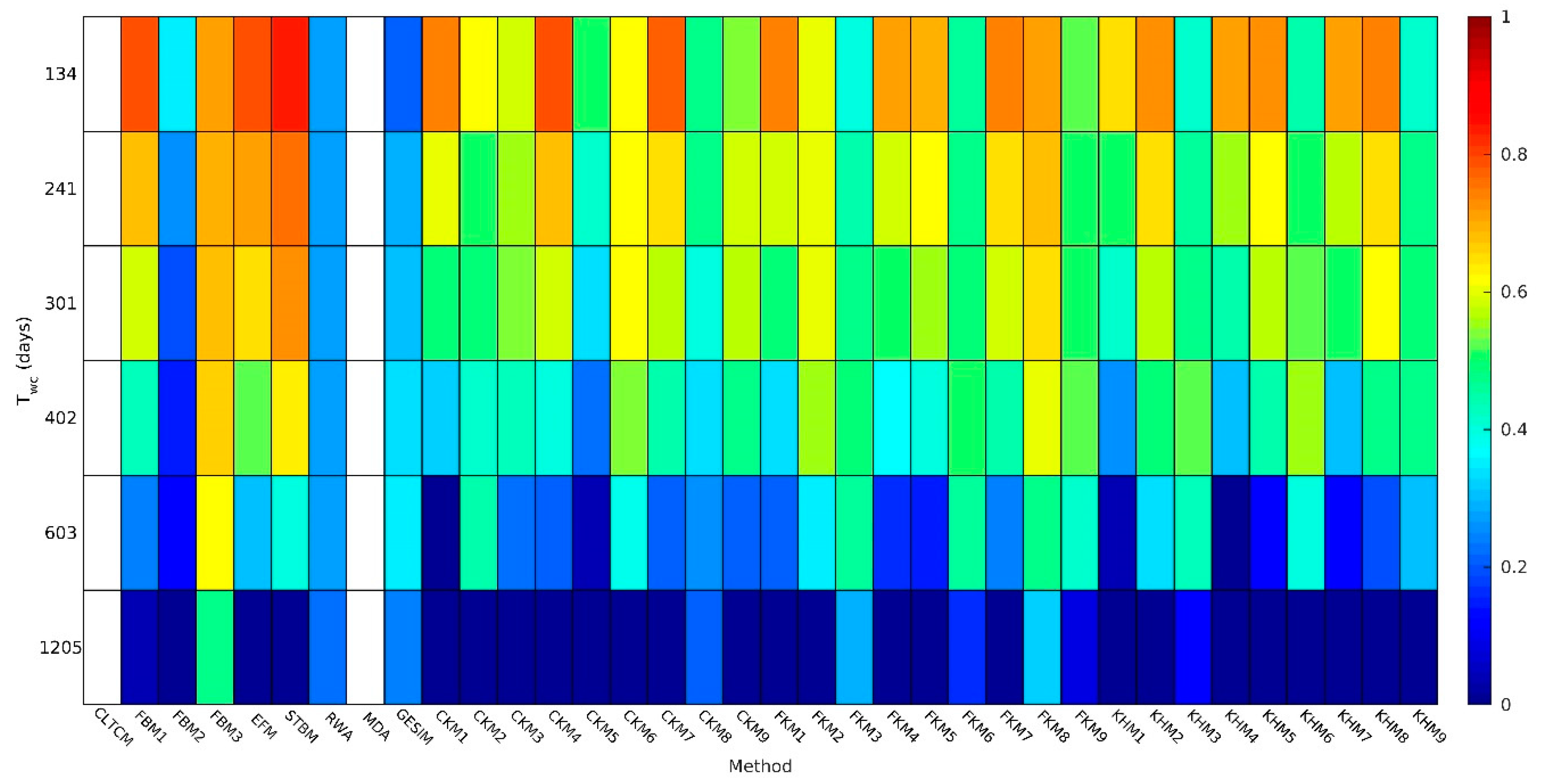
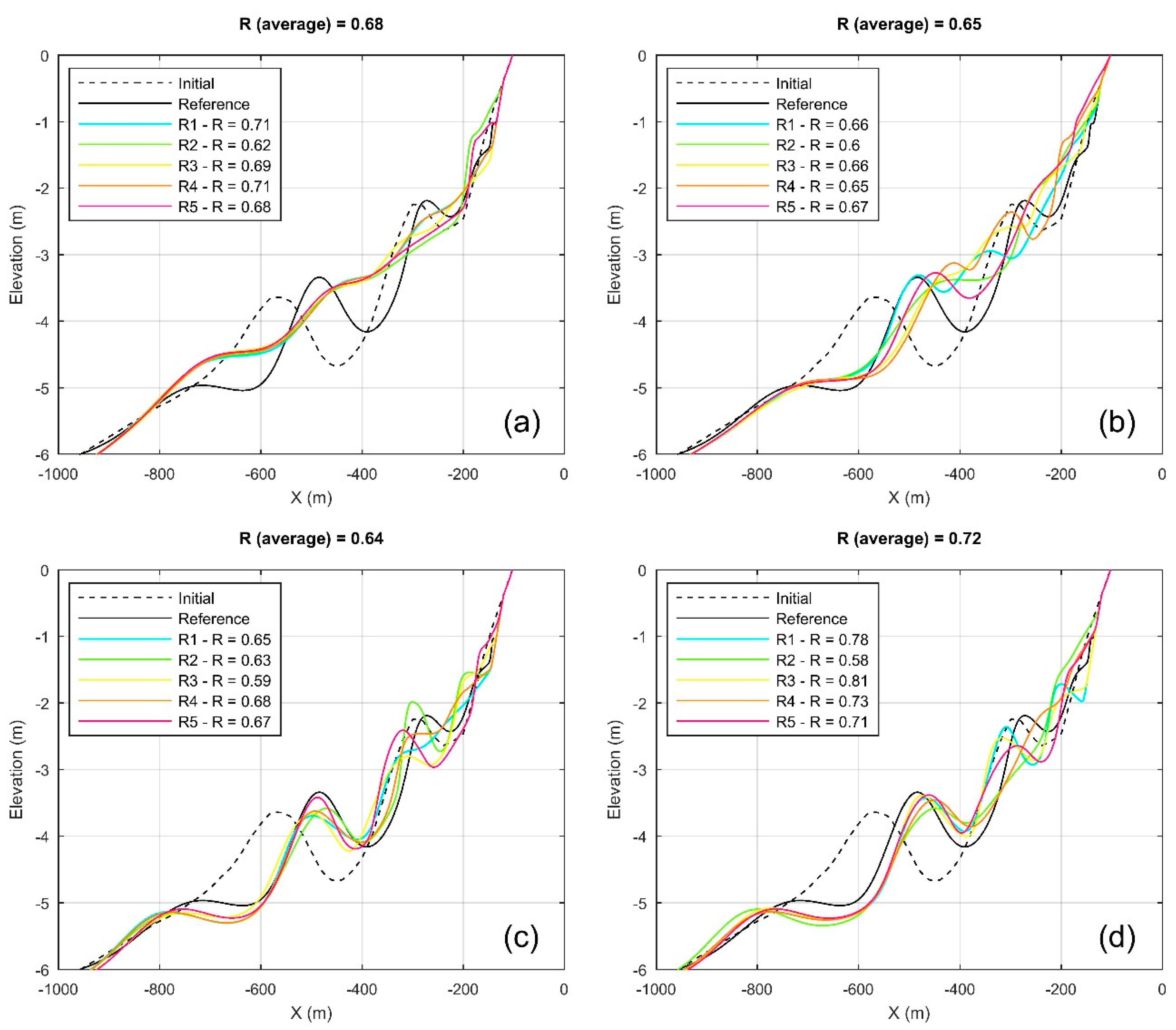
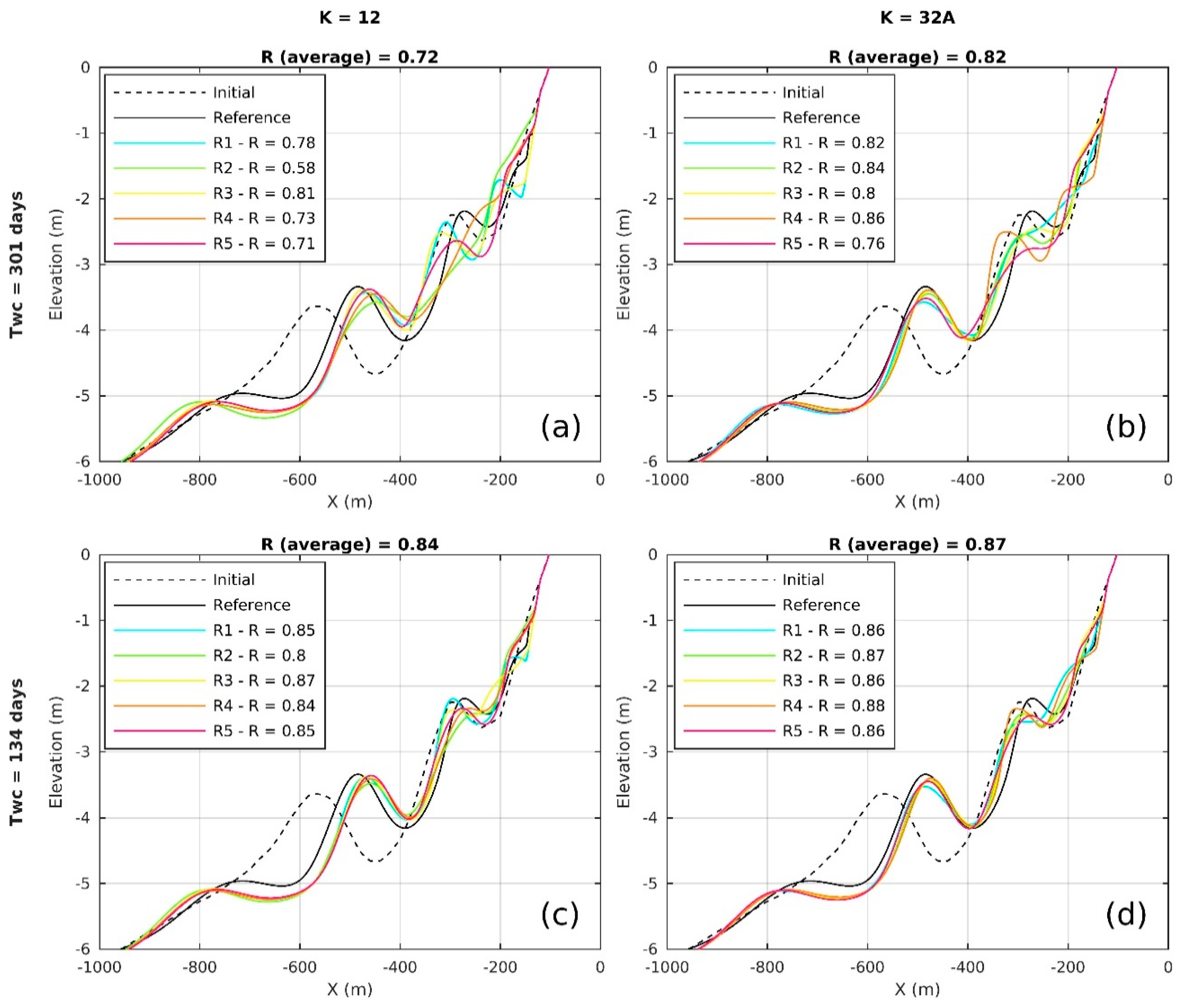
5.1. Performance Evaluation of Input Reduction Methods
5.1.1. Binning Methods
5.1.2. Clustering Methods
5.2. Performance Evaluation of Input Reduction Settings
5.2.1. Number of Wave Conditions in Reduced Climate
5.2.2. Sequencing of Wave Conditions
5.2.3. Duration of Reduced Wave Climate
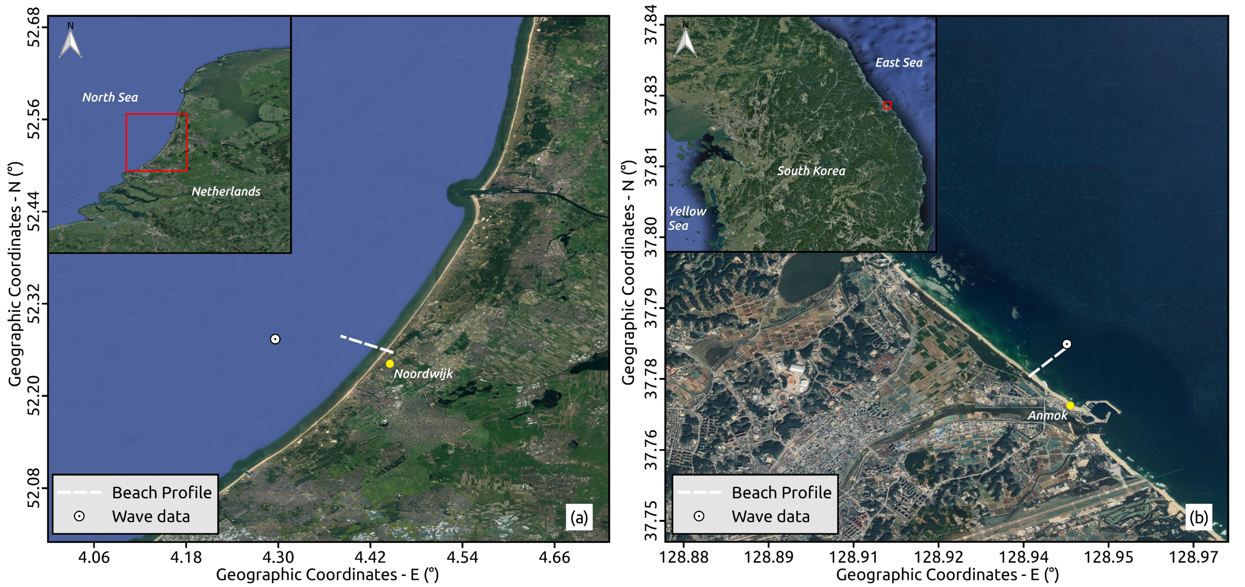
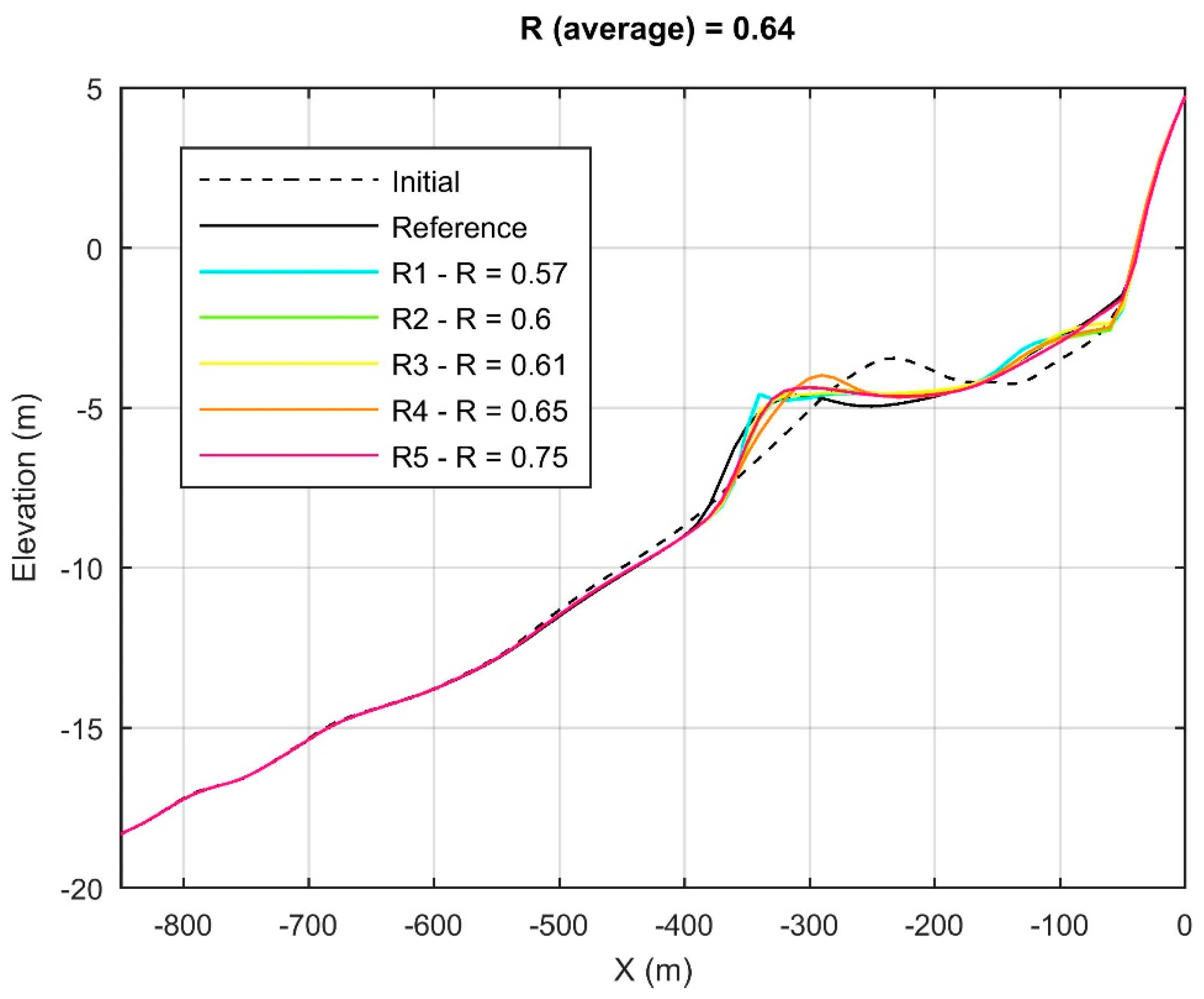
5.3. Validation with Anmok Beach
6. Discussion
7. Conclusions
Author Contributions
Funding
Acknowledgments
Conflicts of Interest
References
- De Vriend, H.J.; Capobianco, M.; Chesher, T.; de Swart, H.E.; Latteux, B.; Stive, M.J.F. Approaches to long-term modelling of coastal morphology: A review. Coast. Eng. 1993, 21, 225–269. [Google Scholar] [CrossRef]
- Walstra, D.J.R.; Hoekstra, R.; Tonnon, P.K.; Ruessink, B.G. Input reduction for long-term morphodynamic simulations in wave-dominated coastal settings. Coast. Eng. 2013, 77, 57–70. [Google Scholar] [CrossRef]
- Benedet, L.; Dobrochinski, J.P.F.; Walstra, D.J.R.; Klein, A.H.F.; Ranasinghe, R. A morphological modeling study to compare different methods of wave climate schematization and evaluate strategies to reduce erosion losses from a beach nourishment project. Coast. Eng. 2016, 112, 69–86. [Google Scholar] [CrossRef]
- Southgate, H.N. The effects of wave chronology on medium and long term coastal morphology. Coast. Eng. 1995, 26, 251–270. [Google Scholar] [CrossRef]
- Van Duin, M.J.P.; Wiersma, N.R.; Walstra, D.J.R.; van Rijn, L.C.; Stive, M.J.F. Nourishing the shoreface: Observations and hindcasting of the Egmond case, The Netherlands. Coast. Eng. 2004, 51, 813–837. [Google Scholar] [CrossRef]
- Brown, J.M.; Davies, A.G. Methods for medium-term prediction of the net sediment transport by waves and currents in complex coastal regions. Cont. Shelf Res. 2009, 29, 1502–1514. [Google Scholar] [CrossRef]
- Lesser, G.R. An Approach to Medium-Term Coastal Morphological Modelling. Ph.D. Thesis, UNESCO-IHE & TUDelft, Delft, The Netherlands, 4 June 2009. [Google Scholar]
- Roelvink, J.A.; Reniers, A.J.H.M. A Guide to Modelling Coastal Morphology; World Scientific Publishing Co. Pte. Ltd.: 5 Toh Tuck Link, Singapore, 2012; pp. 200–215. [Google Scholar]
- Antolinez, J.A.A.; Mendez, F.J.; Camus, P.; Vitousek, S.; Gonzales, E.M.; Ruggiero, P.; Barnard, P. A multisclae climate emulator for long-term morphodynamics (MUSCLE-morpho). J. Geophys. Res. Ocean. 2016, 775–791. [Google Scholar] [CrossRef]
- Walstra, D.J.R.; Reniers, A.J.H.M.; Ranasinghe, R.; Roelvink, J.A.; Ruessink, B.G. On bar growth and decay during interannual net offshore migration. Coast. Eng. 2012, 60, 190–200. [Google Scholar] [CrossRef]
- Ruessink, B.G.; Kuriyama, Y.; Reniers, A.J.H.M.; Roelvink, J.A.; Walstra, D.J.R. Modeling cross-shore sandbar behavior on the timescale of weeks. J. Geophys. Res. Earth Surf. 2007, 112, 1–15. [Google Scholar] [CrossRef]
- Bosboom, J.; Reniers, A.J.H.M.; Luijendijk, A.P. On the perception of morphodynamic model skill. Coast. Eng. 2014, 94, 112–125. [Google Scholar] [CrossRef]
- Olij, D.J.C. Wave Climate Reduction for Medium Term Process Based Morphodynamic Simulations with Application to the Durban Coast. Master’s Thesis, Delft University of Technology, Delft, The Netherlands, 2015; 131p. [Google Scholar]
- Arthur, D.; Vassilvitskii, S.K. Means++: The Advantages of Careful Seeding. Proc. Annu. ACM-SIAM Symp. Discret. Algor. 2007, 8, 1025–1027. [Google Scholar]
- Kennard, R.W.; Stone, L.A. Computer Aided Design of Experiments. Technometrics 1969, 11, 137–148. [Google Scholar] [CrossRef]
- Willett, P. Molecular Diversity Techniques for Chemical Databases. Available online: http://www.informationr.net/ir/2-3/paper19.html (accessed on 11 November 2018).
- Polinsky, A.; Feinstein, R.D.; Shi, S.; Kuki, A. Molecular Diversity and Combinatorial Chemistry. In Libraries and Drug Discovery; American Chemical Society: Washington, DC, USA, 1996; pp. 219–232. [Google Scholar]
- Camus, P.; Mendez, F.J.; Medina, R.; Cofiño, A.S. Analysis of clustering and selection algorithms for the study of multivariate wave climate. Coast. Eng. 2011, 58, 453–462. [Google Scholar] [CrossRef]
- Macqueen, J. Some methods for classification and analysis of multivariate observations. Proc. Fifth Berkeley Symp. Math. Stat. Probab. 1967, 1, 281–297. [Google Scholar]
- Hastie, T.; Tibshirani, R.; Friedman, J. The Elements of Statistical Learning. Math. Intell. 2001, 27, 83–85. [Google Scholar]
- Chang, C.; Lai, J.; Jeng, M. A Fuzzy K-means Clustering Algorithm Using Cluster Center Displacement. J. Inf. Sci. Eng. 2011, 1009, 995–1009. [Google Scholar]
- Zhang, B.; Hsu, M.; Dayal, U. Clustering Algorithm K-Harmonic Means—A Data Clustering Algorithm; Technical Report HPL-1999-124; Hewlett-Packard Labs: Bristol, UK, 1999. [Google Scholar]
- Zhang, B. Generalized K-Harmonic Means—Boosting in Unsupervised Learning; HP Labs Technical Report HPL-2000-137; HP Laboratories: Palo Alto, CA, USA, 2000. [Google Scholar]
- USACE. Shore Protection Maunal; USACE: Washington, DC, USA, 1984. [Google Scholar]
- Grunnet, N.M.; Ruessink, B.G. Morphodynamic response of nearshore bars to a shoreface nourishment. Coast. Eng. 2005, 52, 119–137. [Google Scholar] [CrossRef]


| Type | Method | Variation | Input Variables | Cluster Initiation |
|---|---|---|---|---|
| Binning | Conditions with the Largest Transport Contribution (CLTCM) | CLTCM | - | |
| Fixed Bins (FBM) | FBM1 | - | ||
| FBM2 | - | |||
| FBM3 | - | |||
| Energy Flux (EFM) | EFM | - | ||
| Sediment Transport Bins Method (STBM) | STBM | - | ||
| The Representative Wave Approach (RWA) | RWA | - | ||
| Clustering | Maximum Dissimilarity Algorithm (MDA) | MDA | - | |
| Grouping with Equal Sediment Influence (GESIM) | GESIM | MDA | ||
| Crisp k-means (CKM) | CKM1 | K-means++ | ||
| CKM2 | K-means++ | |||
| CKM3 | K-means++ | |||
| CKM4 | MDA | |||
| CKM5 | MDA | |||
| CKM6 | MDA | |||
| CKM7 | Fixed Bins | |||
| CKM8 | Fixed Bins | |||
| CKM9 | . | Fixed Bins | ||
| Fuzzy k-means (FKM) | FKM1 | K-means++ | ||
| FKM2 | K-means++ | |||
| FKM3 | K-means++ | |||
| FKM4 | MDA | |||
| FKM5 | MDA | |||
| FKM6 | MDA | |||
| FKM7 | Fixed Bins | |||
| FKM8 | Fixed Bins | |||
| FKM9 | Fixed Bins | |||
| K-harmonic means (KHM) | KHM1 | K-means++ | ||
| KHM2 | K-means++ | |||
| KHM3 | K-means++ | |||
| KHM4 | MDA | |||
| KHM5 | MDA | |||
| KHM6 | MDA | |||
| KHM7 | Fixed Bins | |||
| KHM8 | Fixed Bins | |||
| KHM9 | Fixed Bins |
| Parameter | Value |
|---|---|
| Grid Resolution () | 10 m–100 m |
| Time-step () | 0.04167 days |
| Median grain diameter () | 400 μm |
| Breaker-delay () | 1 |
| Angle of repose 1 () | 1.5 |
| Cross-shore location of ϕ1 () | 400 m |
| Angle of repose 2 () | 0.1 |
| Cross-shore location of ϕ2 () | 150 m |
| Current-related roughness () | 0.005593 |
| Wave-related roughness () | 0.00045 |
| Label | Number of Representative Wave Conditions (k) | ndir | nhrms |
|---|---|---|---|
| 8 | 4 | 2 | |
| 10 | 2 | 5 | |
| 16 | 4 | 4 | |
| 24 | 6 | 4 | |
| 24 | 4 | 6 | |
| 24 | 8 | 3 | |
| 32 | 8 | 4 | |
| 32 | 4 | 8 |
| Name | Sequencing Method |
|---|---|
| S1 | Random (five replicates) |
| S2 | Markov Chain |
| S3 | Monte Carlo Markov Chain (five replicates) |
| S4 | Monte Carlo Markov Chain with repetition (five replicates) |
| Duration of Wave Climate (days) | Number of Repetitions |
|---|---|
| Number of Cases (k) | Duration of Wave Climate (Twc) | Number of Transitions (NoT) |
|---|---|---|
© 2019 by the authors. Licensee MDPI, Basel, Switzerland. This article is an open access article distributed under the terms and conditions of the Creative Commons Attribution (CC BY) license (http://creativecommons.org/licenses/by/4.0/).
Share and Cite
de Queiroz, B.; Scheel, F.; Caires, S.; Walstra, D.-J.; Olij, D.; Yoo, J.; Reniers, A.; de Boer, W. Performance Evaluation of Wave Input Reduction Techniques for Modeling Inter-Annual Sandbar Dynamics. J. Mar. Sci. Eng. 2019, 7, 148. https://doi.org/10.3390/jmse7050148
de Queiroz B, Scheel F, Caires S, Walstra D-J, Olij D, Yoo J, Reniers A, de Boer W. Performance Evaluation of Wave Input Reduction Techniques for Modeling Inter-Annual Sandbar Dynamics. Journal of Marine Science and Engineering. 2019; 7(5):148. https://doi.org/10.3390/jmse7050148
Chicago/Turabian Stylede Queiroz, Bruna, Freek Scheel, Sofia Caires, Dirk-Jan Walstra, Derrick Olij, Jeseon Yoo, Ad Reniers, and Wiebe de Boer. 2019. "Performance Evaluation of Wave Input Reduction Techniques for Modeling Inter-Annual Sandbar Dynamics" Journal of Marine Science and Engineering 7, no. 5: 148. https://doi.org/10.3390/jmse7050148
APA Stylede Queiroz, B., Scheel, F., Caires, S., Walstra, D.-J., Olij, D., Yoo, J., Reniers, A., & de Boer, W. (2019). Performance Evaluation of Wave Input Reduction Techniques for Modeling Inter-Annual Sandbar Dynamics. Journal of Marine Science and Engineering, 7(5), 148. https://doi.org/10.3390/jmse7050148