Energy Yield Assessment from Ocean Currents in the Insular Shelf of Cozumel Island

 ,
,  , ,
, , 
 ,
,  ,
, 
Abstract
1. Introduction
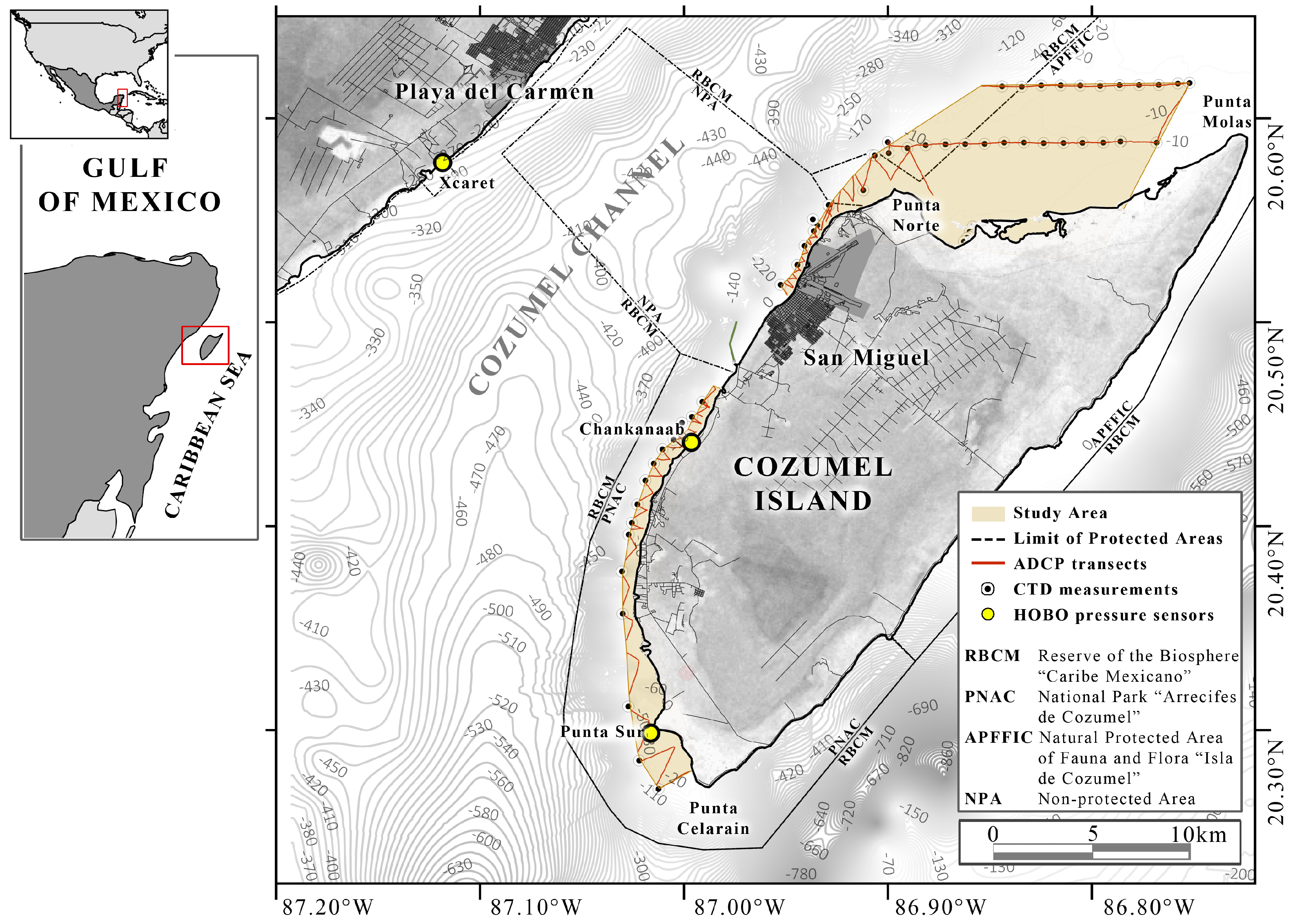
2. Study Area
3. Materials and Methods
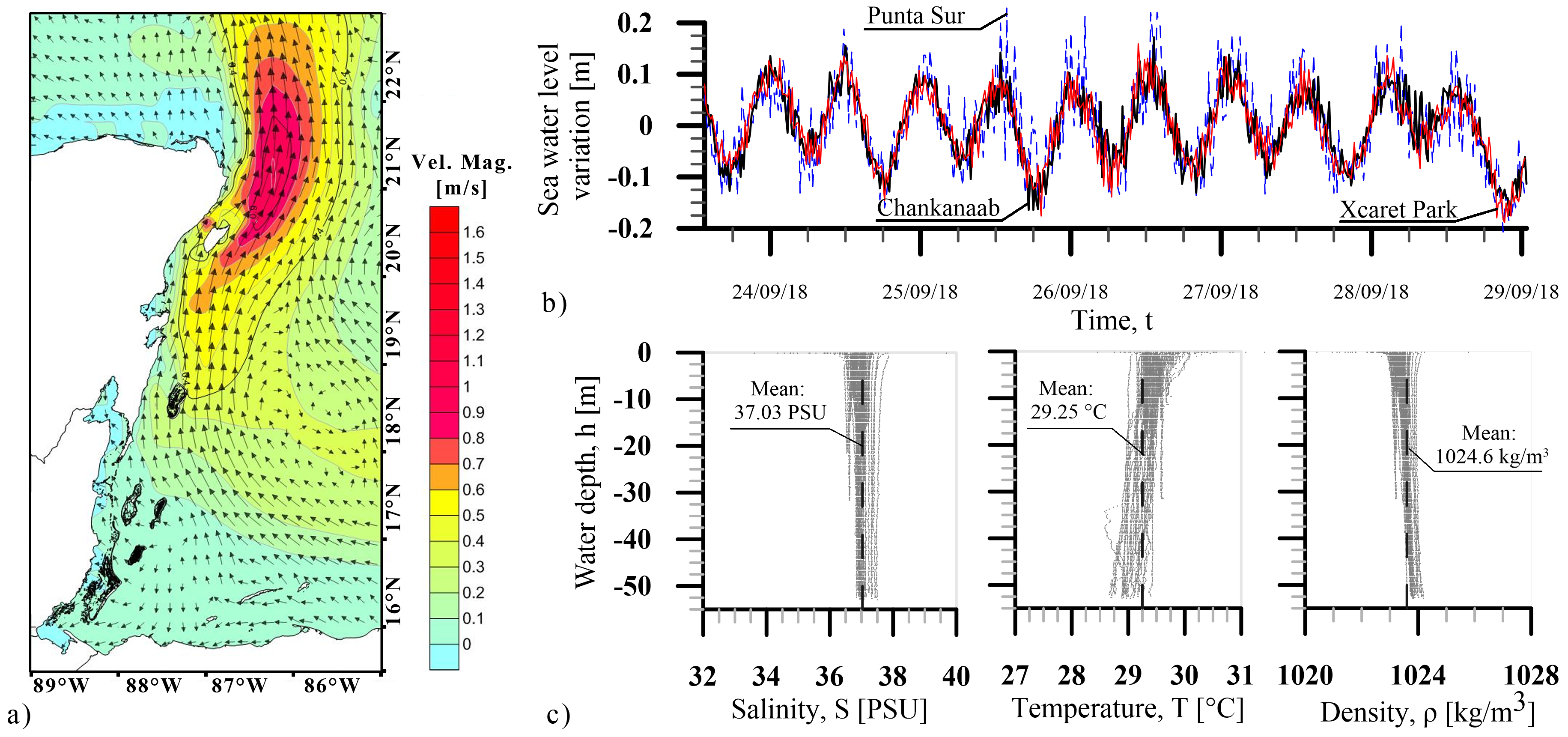
3.1. Field Measurements
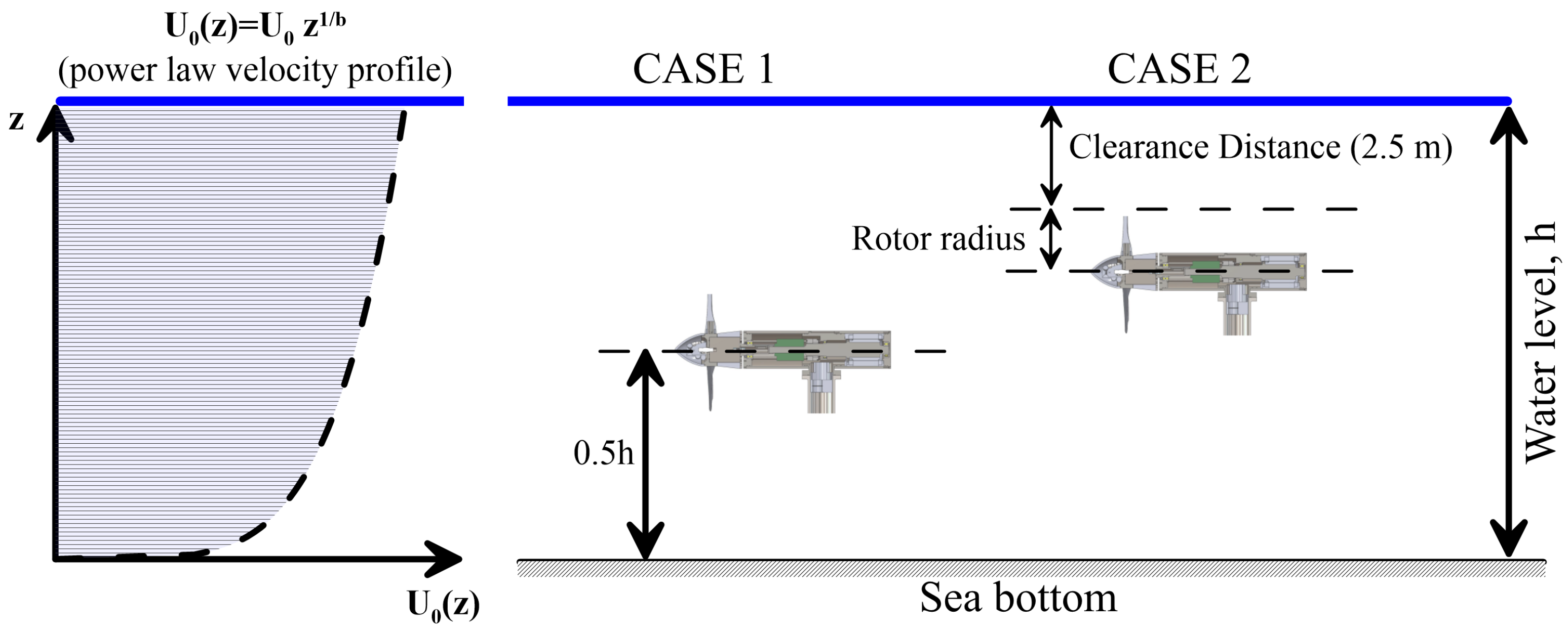
3.2. Analytical Model
4. Results
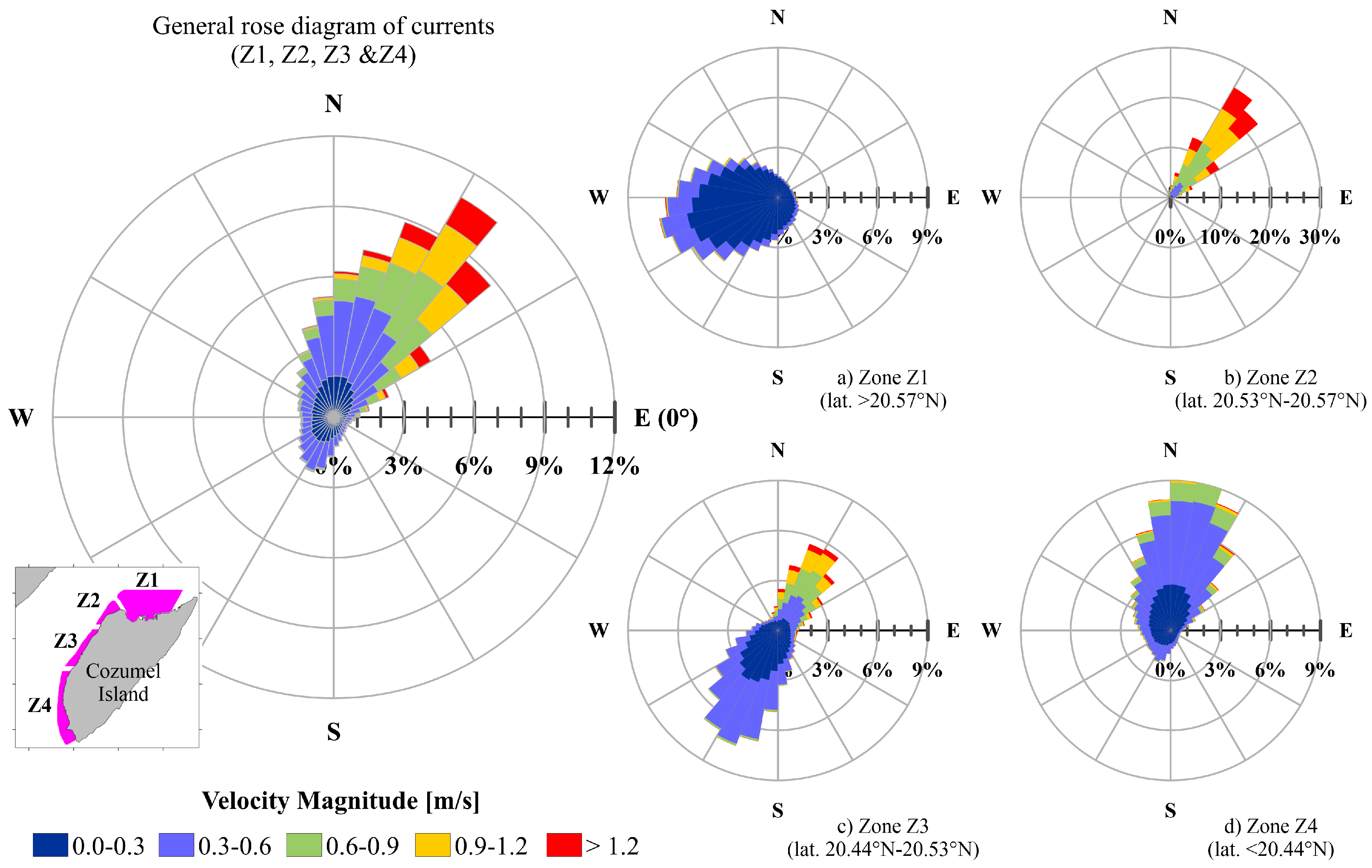
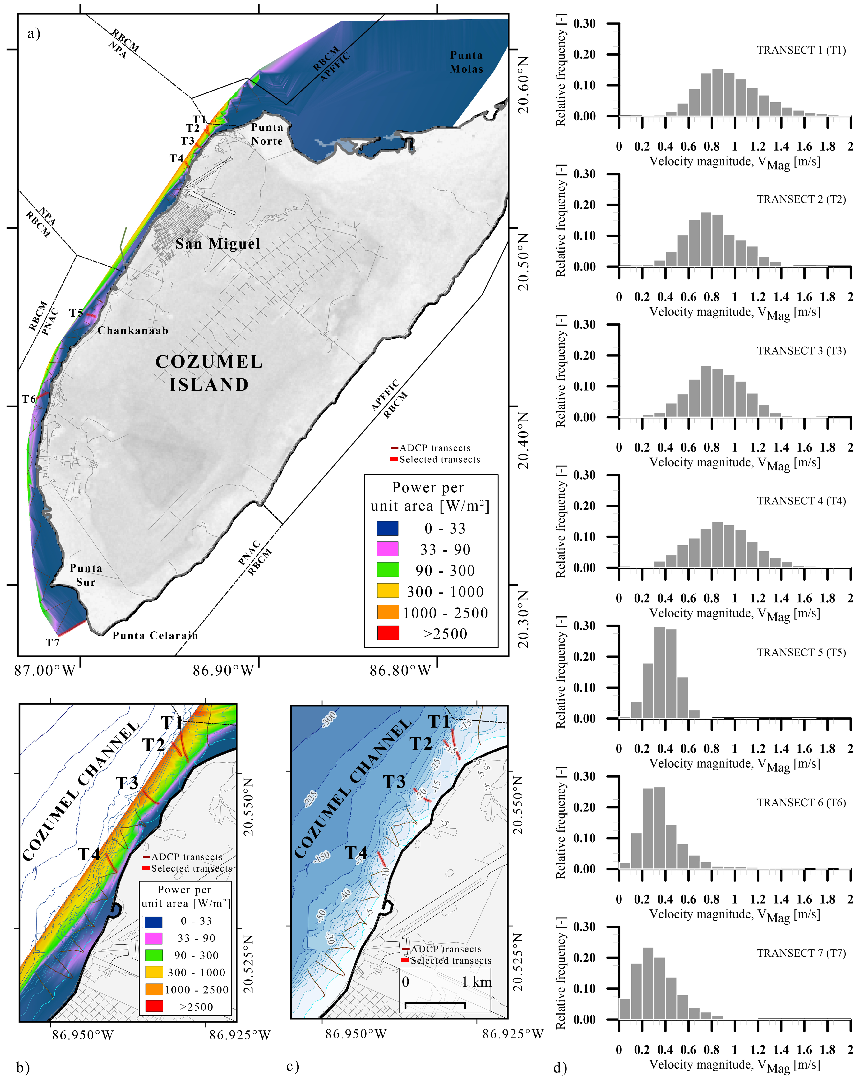
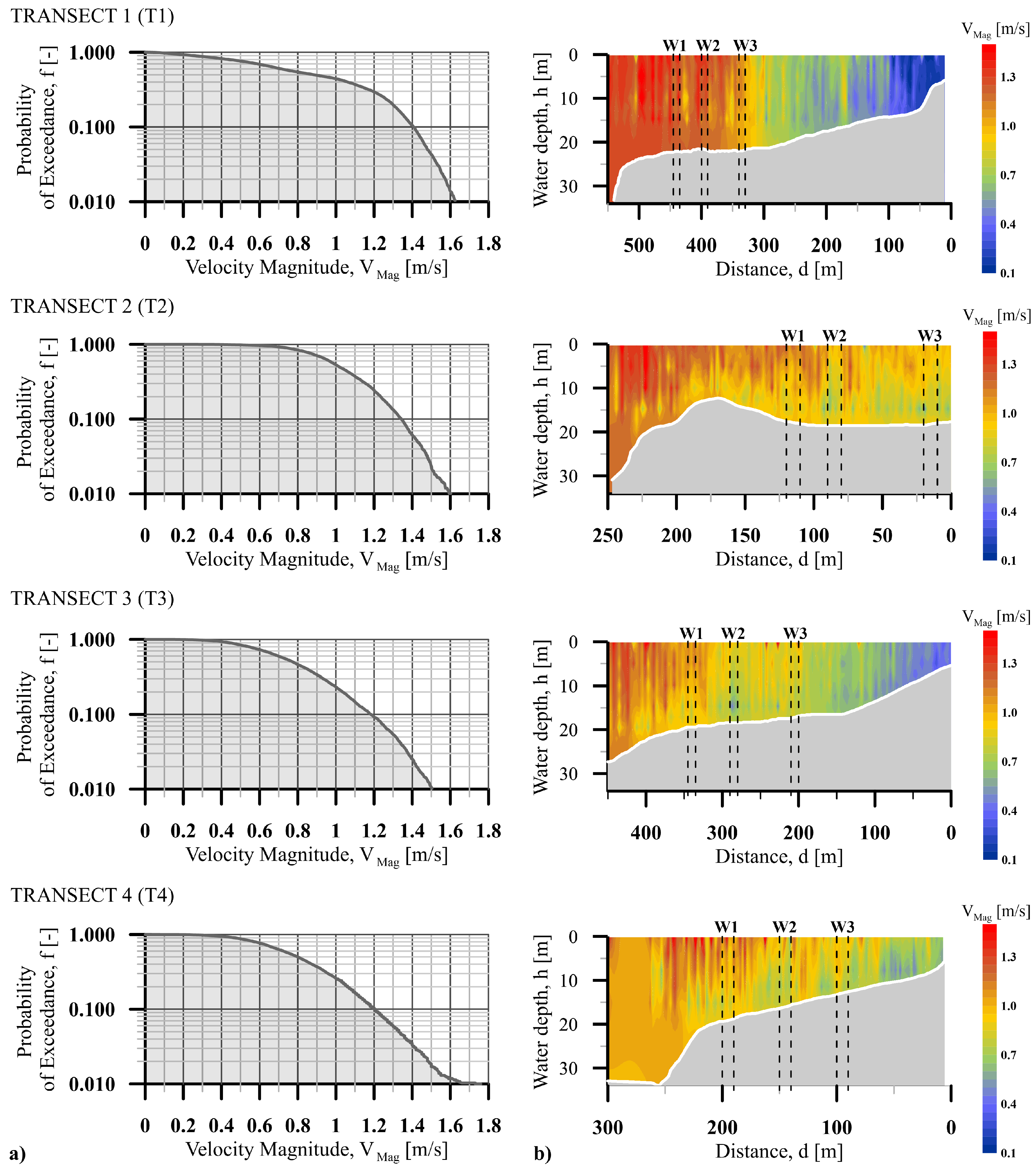
4.1. Flow Velocities and Power Estimation
4.2. Powe Output
5. Discussion and Concluding Remarks
Author Contributions
Acknowledgments
Conflicts of Interest
References
- Jenniches, S. Assessing the regional economic impacts of renewable energy sources—A literature review. Renew. Sustain. Energy Rev. 2018, 93, 35–51. [Google Scholar] [CrossRef]
- Huckerby, J.; Jeffrey, H.; de Andres, A.; Finaly, L. An International Vision for Ocean Energy. Version III, 2nd ed.; Ocean Energy Systems Technology Collaboration Programme: Lisbon, Portugal, 2016; Available online: www.ocean-energy-systems.org (accessed on 13 October 2018).
- Jeffrey, H.; Jay, B.; Winskel, M. Accelerating the development of marine energy: Exploring the prospects, benefits and challenges. Technol. Forecast. Soc. Chang. 2013, 80, 1306–1316. [Google Scholar] [CrossRef]
- Khan, N.; Kalair, A.; Abas, N.; Haider, A. Review of ocean tidal, wave and thermal energy technologies. Renew. Sustain. Energy Rev. 2017, 72, 590–604. [Google Scholar] [CrossRef]
- Matthew, G.J.; Fitch-Roy, O.; Connor, P.; Woodman, B. ICE Report T2. 1.1-Smart Peripheral Territories Transitions: Literature Review and Current Status; Technical Report; University of Exeter: Exeter, UK, 2018. [Google Scholar]
- Uihlein, A.; Magagna, D. Wave and tidal current energy—A review of the current state of research beyond technology. Renew. Sustain. Energy Rev. 2016, 58, 1070–1081. [Google Scholar] [CrossRef]
- Bhuyan, G.S. Harnessing the power of the oceans. IEA OPEN Energy Technol. Bull. 2008, 7, 30–35. [Google Scholar]
- Kerr, D. Marine energy. Philos. Trans. R. Soc. A Math. Phys. Eng. Sci. 2007, 365, 971–992. [Google Scholar] [CrossRef]
- Pelc, R.; Fujita, R.M. Renewable energy from the ocean. Mar. Policy 2002, 26, 471–479. [Google Scholar] [CrossRef]
- Nova Innovation Ltd. Nova M100-D. Available online: https://www.novainnovation.com/nova-m100-d (accessed on 13 March 2019).
- Simec Atlantis Energy. Meygen. Available online: https://simecatlantis.com/ (accessed on 13 March 2019).
- Zhou, Z.; Benbouzid, M.; Frédéric Charpentier, J.; Scuiller, F.; Tang, T. A review of energy storage technologies for marine current energy systems. Renew. Sustain. Energy Rev. 2013, 18, 390–400. [Google Scholar] [CrossRef]
- Yang, X.; Haas, K.A.; Fritz, H.M. Theoretical Assessment of Ocean Current Energy Potential for the Gulf Stream System. Mar. Technol. Soc. J. 2013, 47, 101–112. [Google Scholar] [CrossRef]
- Haas, K.; Yang, X.; Neary, V.; Gunawan, B. Ocean Current Energy Resource Assessment for the Gulf Stream System: The Florida Current. In Marine Renewable Energy; Springer International Publishing: Cham, Switzerland, 2017; pp. 217–236. [Google Scholar]
- Hanson, H.P. Gulf Stream energy resources: North Atlantic flow volume increases create more power. Ocean Eng. 2014, 87, 78–83. [Google Scholar] [CrossRef]
- Yang, X.; Haas, K.A.; Fritz, H.M. Evaluating the potential for energy extraction from turbines in the gulf stream system. Renew. Energy 2014, 72, 12–21. [Google Scholar] [CrossRef]
- Athié, G.; Candela, J.; Sheinbaum, J.; Badan, A.; Ochoa, J. Yucatan Current variability through the Cozumel and Yucatan channels. Cienc. Mar. 2011, 37, 471–492. [Google Scholar] [CrossRef]
- Carrillo, L.; Johns, E.; Smith, R.; Lamkin, J.; Largier, J. Pathways and Hydrography in the Mesoamerican Barrier Reef System Part 1: Circulation. Cont. Shelf Res. 2015, 109, 164–176. [Google Scholar] [CrossRef]
- Orhan, K.; Mayerle, R.; Pandoe, W.W. Assesment of Energy Production Potential from Tidal Stream Currents in Indonesia. Energy Procedia 2015, 76, 7–16. [Google Scholar] [CrossRef]
- Ghefiri, K.; Garrido, A.; Rusu, E.; Bouallègue, S.; Haggège, J.; Garrido, I. Fuzzy Supervision Based-Pitch Angle Control of a Tidal Stream Generator for a Disturbed Tidal Input. Energies 2018, 11, 2989. [Google Scholar] [CrossRef]
- Encarnacion, J.; Johnstone, C. Preliminary Design of a Horizontal Axis Tidal Turbine for Low-Speed Tidal Flow. In Proceedings of the 4th Asian Wave and Tidal Energy Conference, Taipei, Taiwan, 9–13 September 2018. [Google Scholar]
- Chávez, G.; Candela, J.; Ochoa, J. Subinertial flows and transports in Cozumel Channel. J. Geophys. Res. Ocean. 2003, 108. [Google Scholar] [CrossRef]
- Ochoa, J.; Candela, J.; Badan, A.; Sheinbaum, J. Ageostrophic fluctuations in Cozumel channel. J. Geophys. Res. C Ocean. 2005, 110, 1–16. [Google Scholar] [CrossRef]
- Abascal, A.J. Analysis of flow variability in the Yucatan Channel. J. Geophys. Res. 2003, 108, 3381. [Google Scholar] [CrossRef]
- Cetina, P.; Candela, J.; Sheinbaum, J.; Ochoa, J.; Badan, A. Circulation along the Mexican Caribbean coast. J. Geophys. Res. C Ocean. 2006, 111. [Google Scholar] [CrossRef]
- Kjerfve, B. Tides of the Caribbean Sea. J. Geophys. Res. 1981, 86, 4243. [Google Scholar] [CrossRef]
- APIQroo. Manifestación de Impacto Ambiental-Modalidad Particular; Proyecto Marina Cozumel: Carretera Costera, Mexico, 2018. [Google Scholar]
- INEGI. Censo y Conteos de Población y Vivienda; Instituto Nacional de Estadística y Geografía: Quintana Roo, Mexico, 2018. [Google Scholar]
- SENER-World Bank-ESMAP. Evaluación Rápida del uso de Energía, Cozumel, Quintana Roo, México; Technical Report; Secretaría de Energía (SENER), World Bank, Programa de Asistencia para la Gestión del Sector de Energía (ESMAP): Mexico City, Mexico, 2015. [Google Scholar]
- SEDETUR. Indicadores Turísticos 2017. Available online: https://www.qroo.gob.mx/sedetur/indicadores-turisticos (accessed on 13 March 2019).
- Palafox-Muñoz, A.; Zizumbo-Villarreal, L. Distribución territorial y turismo en Cozumel, Estado de Quintana Roo, México. Gestión Turística 2009, 11, 69–88. [Google Scholar] [CrossRef]
- DOF. Decreto por el que se Pretende Declarar Como Área Natural Protegida con el Carácter de Reserva de la Biosfera a la Región Conocida Como Caribe Mexicano. Available online: http://dof.gob.mx/notadetalle.php?codigo=5464450fecha=07/12/2016 (accessed on 13 March 2019).
- DOF. Decreto por el que se Declara Área Natural Protegida, con el Carácter de Area de Protección de Flora y Fauna, la Porción norte y la Franja Costera Oriental, Terrestres y Marinas de la Isla de Cozumel, Municipio de Cozumel, Estado de Quintana Roo. Available online: http://www.dof.gob.mx/notadetalle.php?codigo=5270007fecha=25/09/2012 (accessed on 13 March 2019).
- DOF. Decreto por el que se Declara Área Natural Protegida, con el Carácter de Parque Marino Nacional, la zona Conocida Como Arrecifes de Cozumel. Available online: http://dof.gob.mx/notadetalle.php?codigo=4892806fecha=19/07/1996 (accessed on 13 March 2019).
- Red Nacional de Sistemas Estatales. Áreas Naturales Protegidas—Decretos de ANPs Quintana Roo. Available online: https://www.anpsestatales.mx/anps.php?tema=3estado=25 (accessed on 13 March 2019).
- Martínez, S.; Carrillo, L.; Marinone, S. Potential connectivity between marine protected areas in the Mesoamerican Reef for two species of virtual fish larvae: Lutjanus analis and Epinephelus striatus. Ecol. Indic. 2019, 102, 10–20. [Google Scholar] [CrossRef]
- Alvera-Azcárate, A.; Barth, A.; Weisberg, R.H. The surface circulation of the Caribbean Sea and the Gulf of Mexico as inferred from satellite altimetry. J. Phys. Oceanogr. 2009, 39, 640–657. [Google Scholar] [CrossRef]
- Rousset, C.; Beal, L.M. Observations of the Florida and Yucatan Currents from a Caribbean cruise ship. J. Phys. Oceanogr. 2010, 40, 1575–1581. [Google Scholar] [CrossRef]
- TELEDYNE Marine. RiverPro ADCP -RD Instruments-. Available online: http://www.teledynemarine.com/riverpro-adcp?ProductLineID=13 (accessed on 12 March 2019).
- Secretaría de Marina. Catalogo de Cartas y Publicaciones Náuticas; Secretaría de Marina: Mexico City, Mexico, 2019; p. 39. [Google Scholar]
- The SciPy community. Optimization (scipy.optimize). Available online: https://docs.scipy.org/doc/scipy/reference/tutorial/optimize.html (accessed on 12 March 2019).
- Shen, W.Z.; Mikkelsen, R.; Sørensen, J.N.; Bak, C. Tip loss corrections for wind turbine computations. Wind Energy 2005, 8, 457–475. [Google Scholar] [CrossRef]
- Manwell, J.F.; McGowan, J.G.; Rogers, A.L. Wind Energy Explained: Theory, Design and Application; John Wiley & Sons, Ltd.: Chichester, UK, 2009. [Google Scholar]
- Spera, D. Wind Turbine Technology: Fundamental Concepts in Wind Turbine Engineering, 2nd ed.; ASME: New York, NY, USA, 2009. [Google Scholar]
- Frost, C.H.; Evans, P.S.; Harrold, M.J.; Mason-Jones, A.; O’Doherty, T.; O’Doherty, D.M. The impact of axial flow misalignment on a tidal turbine. Renew. Energy 2017, 113, 1333–1344. [Google Scholar] [CrossRef]
- Sutherland, D.; Ordonez-Sanchez, S.; Belmont, M.R.; Moon, I.; Steynor, J.; Davey, T.; Bruce, T. Experimental optimisation of power for large arrays of cross-flow tidal turbines. Renew. Energy 2018, 116, 685–696. [Google Scholar] [CrossRef]
- Mycek, P.; Gaurier, B.; Germain, G.; Pinon, G.; Rivoalen, E. Experimental study of the turbulence intensity effects on marine current turbines behaviour. Part I: One single turbine. Renew. Energy 2014, 66, 729–746. [Google Scholar] [CrossRef]
- Harding, S.; Bryden, I. Directionality in prospective Northern UK tidal current energy deployment sites. Renew. Energy 2012, 44, 474–477. [Google Scholar] [CrossRef]
- Laws, N.D.; Epps, B.P. Hydrokinetic energy conversion: Technology, research, and outlook. Renew. Sustain. Energy Rev. 2016, 57, 1245–1259. [Google Scholar] [CrossRef]
- Sandoval Vizcaíno, S. Dinámica de corrientes marinas. In Biodiversidad acuática de la Isla de Cozumel; Mejía-Ortíz, L.M., Ed.; Universidad de Quintana Roo-Plaza Y Valdés: Mexico City, Mexico, 2007; Chapter 3. [Google Scholar]
- Gallrein, A.; Smith, S. Cozumel: Dive Guide & Log Book; Underwater Editions: Cozumel, Quintana Roo, Mexico, 2003. [Google Scholar]
- Muckelbauer, G. The shelf of Cozumel, Mexico: Topography and organisms. Facies 1990, 23, 201–239. [Google Scholar] [CrossRef]
- Palafox-Muñoz, A.; Segrado-Pavón, R. Capacidad de carga turística: Alternativa para el Desarrollo Sustentable de Cozumel. Tur. Desenvolv. 2008, 10, 109. [Google Scholar]
- Ordonez-Sanchez, S.; Porter, K.; Frost, C.; Allmark, M.; Johnstone, C.; O’Doherty, T. Effects of Wave-Current Interactions on the Performance of Tidal Stream Turbines. In Proceedings of the 3rd Asian Wave and Tidal Energy Conference, Singapore, 24–28 October 2016. [Google Scholar]
- Irena. Innovation Outlook: Offshore Wind; Technical Report; International Renewable Energy Agency: Abu Dhabi, UAE, 2016. [Google Scholar]
- Vennell, R.; Funke, S.W.; Draper, S.; Stevens, C.; Divett, T. Designing large arrays of tidal turbines: A synthesis and review. Renew. Sustain. Energy Rev. 2015, 41, 454–472. [Google Scholar] [CrossRef]
- Blackmore, T.; Myers, L.E.; Bahaj, A.S. Effects of turbulence on tidal turbines: Implications to performance, blade loads, and condition monitoring. Int. J. Mar. Energy 2016, 14, 1–26. [Google Scholar] [CrossRef]
- Nevalainen, T.M. The Effect of uNsteady Sea Conditions on Tidal Stream Turbine Loads and Durability. Ph.D. Thesis, University of Strathclyde, Glasgow, Scotland, 2016. [Google Scholar]
- Liu, Y.; Yu, S.; Zhu, Y.; Wang, D.; Liu, J. Modeling, planning, application and management of energy systems for isolated areas: A review. Renew. Sustain. Energy Rev. 2018, 82, 460–470. [Google Scholar] [CrossRef]
- Mendoza-Vizcaino, J.; Sumper, A.; Galceran-Arellano, S. PV, wind and storage integration on small islands for the fulfilment of the 50-50 renewable electricity generation target. Sustainability 2017, 9, 905. [Google Scholar] [CrossRef]
- Mendoza-Vizcaino, J.; Sumper, A.; Sudria-Andreu, A.; Ramirez, J.M. Renewable technologies for generation systems in islands and their application to Cozumel Island, Mexico. Renew. Sustain. Energy Rev. 2016, 64, 348–361. [Google Scholar] [CrossRef]


| Transect | Latitude (°) | Longitude (°) | Length (m) | Depth-Averaged Vel. (m s−1) | Depth-Averaged Vel. Fluct. (σ) (m s−1) | Direction * (θ) (°) | Direction Fluct. (σ) (°) | |
|---|---|---|---|---|---|---|---|---|
| T1 | Start | 20.5524 | −86.9279 | |||||
| End | 20.5567 | −86.9290 | 489.5 | 0.98 | 0.30 | 50.00 | 14.49 | |
| T2 | Start | 20.5529 | −86.9288 | |||||
| End | 20.5549 | −86.9302 | 250.0 | 1.03 | 0.24 | 48.60 | 13.05 | |
| T3 | Start | 20.5452 | −86.9326 | |||||
| End | 20.5472 | −86.9351 | 340.8 | 1.04 | 0.24 | 48.34 | 13.13 | |
| T4 | Start | 20.5138 | −86.9496 | |||||
| End | 20.5179 | −86.9524 | 317.8 | 0.83 | 0.30 | 62.74 | 24.25 | |
| T5 | Start | 20.4515 | −86.9962 | |||||
| End | 20.4504 | −86.9919 | 470.6 | 0.39 | 0.12 | 267.23 | 33.80 | |
| T6 | Start | 20.4041 | −87.0246 | |||||
| End | 20.4076 | −87.0187 | 722.4 | 0.37 | 0.19 | 70.03 | 31.96 | |
| T7 | Start | 20.2797 | −86.9974 | |||||
| End | 20.2714 | −87.0119 | 1778.7 | 0.34 | 0.20 | 73.09 | 43.94 | |
| Average | 624.3 | 0.71 | 0.23 | 88.58 | 24.95 |
| Transect ID | Window | (m/s) | b | Water Depth (m) | Distance * (m) |
|---|---|---|---|---|---|
| 1 | 0.85 | 4.99 | 19.43 | 105–115 | |
| T1 | 2 | 0.85 | 3.08 | 18.52 | 150–160 |
| 3 | 0.80 | 5.43 | 17.88 | 210–220 | |
| 1 | 1.13 | 3.11 | 17.83 | 130–1405 | |
| T2 | 2 | 1.12 | 2.82 | 18.47 | 160–170 |
| 3 | 1.16 | 3.05 | 18.15 | 230–240 | |
| 1 | 0.86 | 4.99 | 19.43 | 105–115 | |
| T3 | 2 | 0.79 | 6.89 | 18.47 | 160–170 |
| 3 | 0.81 | 2.60 | 17.62 | 240–250 | |
| 1 | 0.88 | 6.14 | 19.06 | 100–110 | |
| T4 | 2 | 0.74 | 6.26 | 16.07 | 150–160 |
| 3 | 0.87 | 4.32 | 12.86 | 200–210 |
| Transect ID | Window 1 | Window 2 | Window 3 | Total Power (kW) | |
|---|---|---|---|---|---|
| Case 1—Bottom Mounted | |||||
| T1 | Power (kW) | 1.69 | 1.29 | 1.46 | 4.43 |
| CP | 0.27 | 0.21 | 0.28 | ||
| T2 | Power (kW) | 3.19 | 2.68 | 3.01 | 8.87 |
| CP | 0.20 | 0.19 | 0.21 | ||
| T3 | Power (kW) | 1.75 | 1.50 | 1.02 | 4.27 |
| CP | 0.27 | 0.31 | 0.19 | ||
| T4 | Power (kW) | 2.02 | 1.21 | 1.70 | 4.93 |
| CP | 0.30 | 0.30 | 0.25 | ||
| Case 2—Floating Device | |||||
| T1 | Power (kW) | 2.17 | 1.92 | 1.80 | 5.89 |
| CP | 0.35 | 0.31 | 0.35 | ||
| T2 | Power (kW) | 4.75 | 4.17 | 4.42 | 13.34 |
| CP | 0.30 | 0.30 | 0.30 | ||
| T3 | Power (kW) | 2.24 | 1.78 | 1.53 | 5.56 |
| CP | 0.35 | 0.37 | 0.28 | ||
| T4 | Power (kW) | 2.45 | 1.42 | 1.98 | 5.86 |
| CP | 0.36 | 0.35 | 0.30 | ||
| Number of Turbines | 3 (n = 1) | 6 (n = 2) | 9 (n = 3) | 12 (n = 4) | 15 (n = 5) |
|---|---|---|---|---|---|
| Centre to Centre Distance * | 50.0 (10D) | 20.0 (4D) | 12.5 (2.5D) | 9.1 (1.8D) | 7.1 (1.4D) |
| Transect ID | Case 1—Bottom Mounted | ||||
| T1 | 4.43 | 8.87 | 13.30 | 17.74 | 22.17 |
| T2 | 8.87 | 17.75 | 26.62 | 35.49 | 44.36 |
| T3 | 4.27 | 8.53 | 12.80 | 17.07 | 21.34 |
| T4 | 4.93 | 9.87 | 14.80 | 19.73 | 24.66 |
| Total Power Output (kW) | 22.5 | 45.02 | 67.52 | 90.03 | 112.53 |
| Transect ID | Case 2—Floating device | ||||
| T1 | 5.89 | 11.79 | 17.68 | 23.57 | 29.47 |
| T2 | 13.34 | 26.68 | 40.02 | 53.36 | 66.70 |
| T3 | 5.56 | 11.12 | 16.67 | 22.23 | 27.79 |
| T4 | 5.86 | 11.72 | 17.58 | 23.44 | 29.30 |
| Total Power Output (kW) | 30.65 | 61.31 | 91.95 | 122.6 | 153.26 |
© 2019 by the authors. Licensee MDPI, Basel, Switzerland. This article is an open access article distributed under the terms and conditions of the Creative Commons Attribution (CC BY) license (http://creativecommons.org/licenses/by/4.0/).
Share and Cite
Alcérreca-Huerta, J.C.; Encarnacion, J.I.; Ordoñez-Sánchez, S.; Callejas-Jiménez, M.; Gallegos Diez Barroso, G.; Allmark, M.; Mariño-Tapia, I.; Silva Casarín, R.; O’Doherty, T.; Johnstone, C.; et al. Energy Yield Assessment from Ocean Currents in the Insular Shelf of Cozumel Island. J. Mar. Sci. Eng. 2019, 7, 147. https://doi.org/10.3390/jmse7050147
Alcérreca-Huerta JC, Encarnacion JI, Ordoñez-Sánchez S, Callejas-Jiménez M, Gallegos Diez Barroso G, Allmark M, Mariño-Tapia I, Silva Casarín R, O’Doherty T, Johnstone C, et al. Energy Yield Assessment from Ocean Currents in the Insular Shelf of Cozumel Island. Journal of Marine Science and Engineering. 2019; 7(5):147. https://doi.org/10.3390/jmse7050147
Chicago/Turabian StyleAlcérreca-Huerta, Juan Carlos, Job Immanuel Encarnacion, Stephanie Ordoñez-Sánchez, Mariana Callejas-Jiménez, Gabriel Gallegos Diez Barroso, Matthew Allmark, Ismael Mariño-Tapia, Rodolfo Silva Casarín, Tim O’Doherty, Cameron Johnstone, and et al. 2019. "Energy Yield Assessment from Ocean Currents in the Insular Shelf of Cozumel Island" Journal of Marine Science and Engineering 7, no. 5: 147. https://doi.org/10.3390/jmse7050147
APA StyleAlcérreca-Huerta, J. C., Encarnacion, J. I., Ordoñez-Sánchez, S., Callejas-Jiménez, M., Gallegos Diez Barroso, G., Allmark, M., Mariño-Tapia, I., Silva Casarín, R., O’Doherty, T., Johnstone, C., & Carrillo, L. (2019). Energy Yield Assessment from Ocean Currents in the Insular Shelf of Cozumel Island. Journal of Marine Science and Engineering, 7(5), 147. https://doi.org/10.3390/jmse7050147