Estimation of a Mechanical Recovery System’s Oil Recovery Capacity by Considering Boom Loss


Abstract
1. Introduction
2. Methods
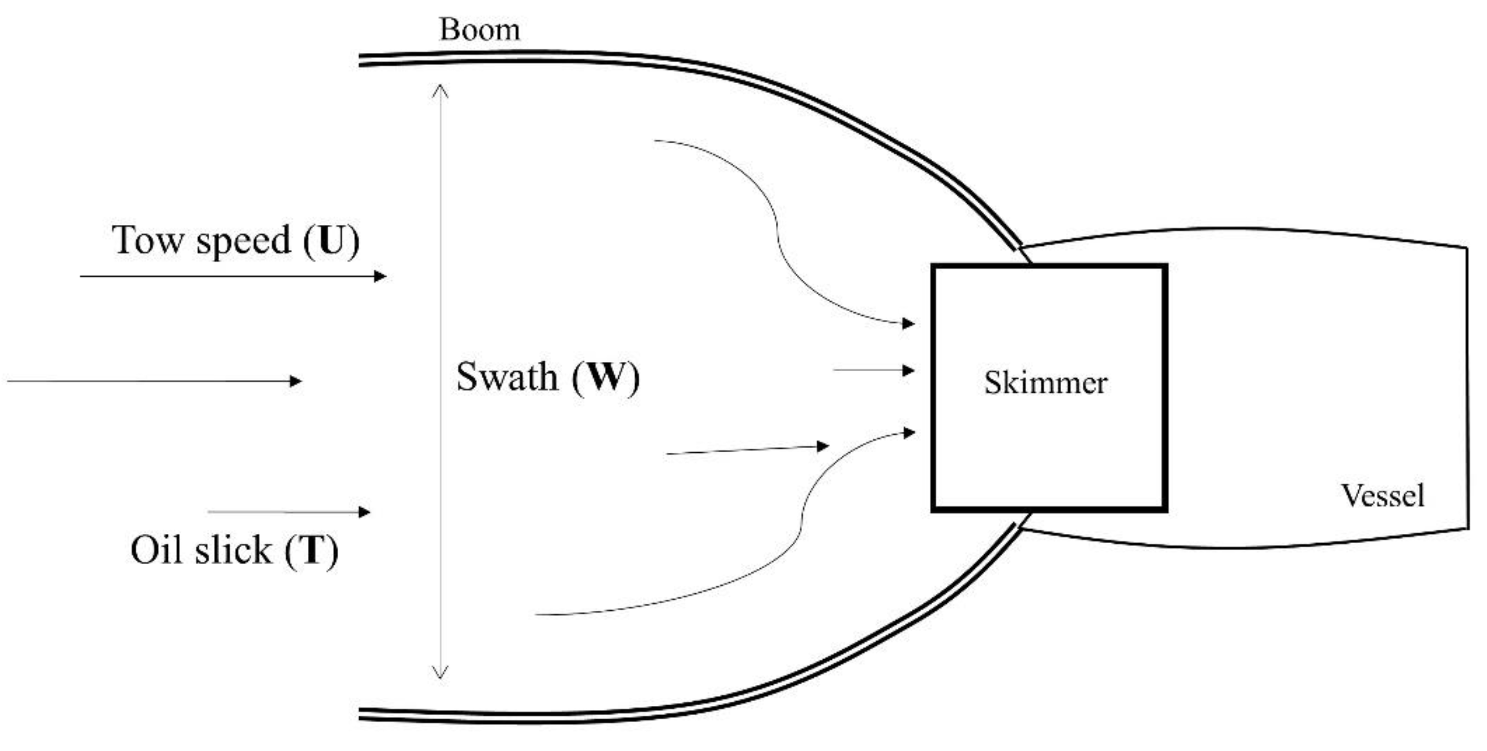
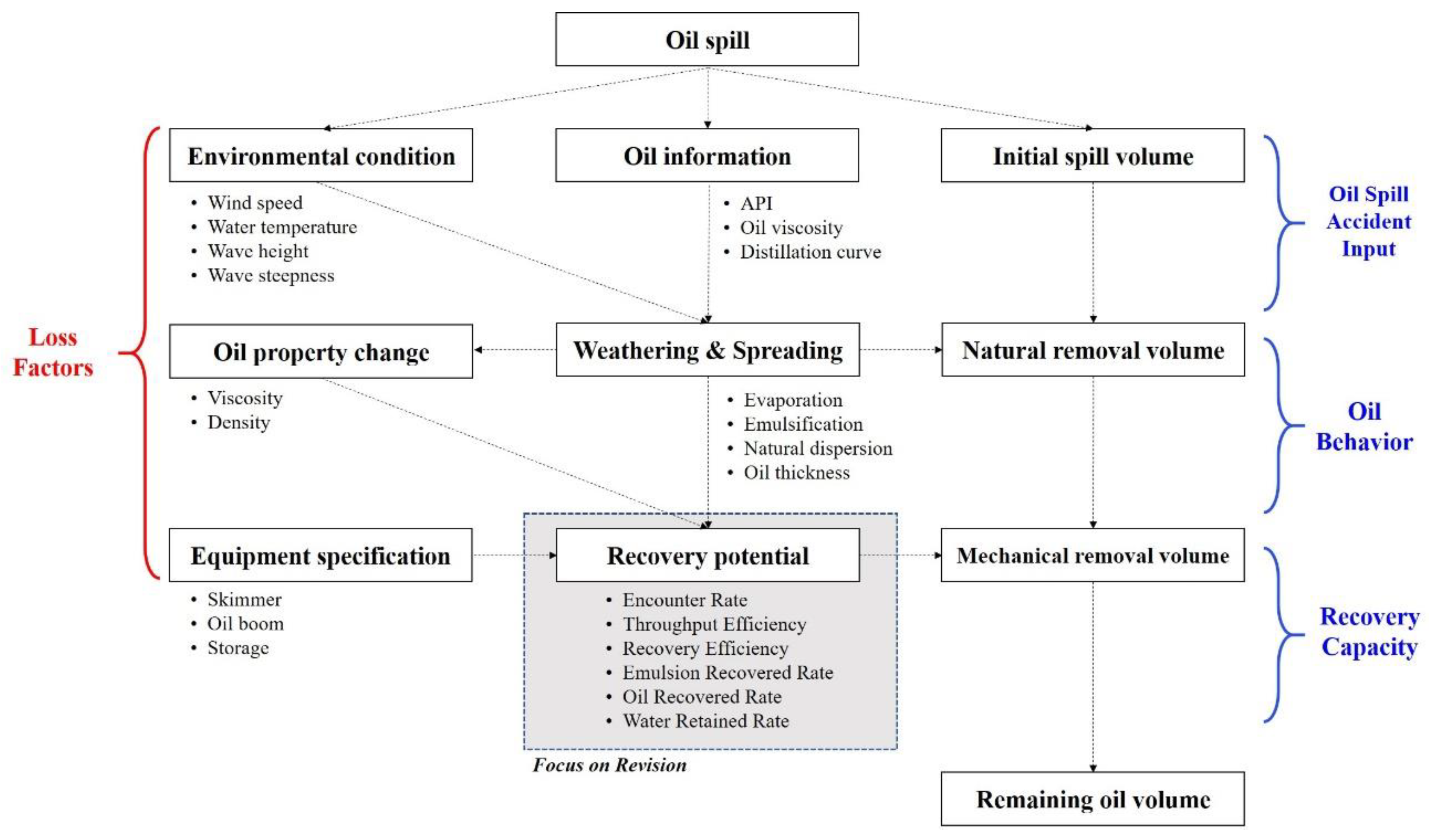
2.1. Recovery Potential Estimation Model Based on the Encounter Rate
2.2. Quantification of Oil Boom Loss
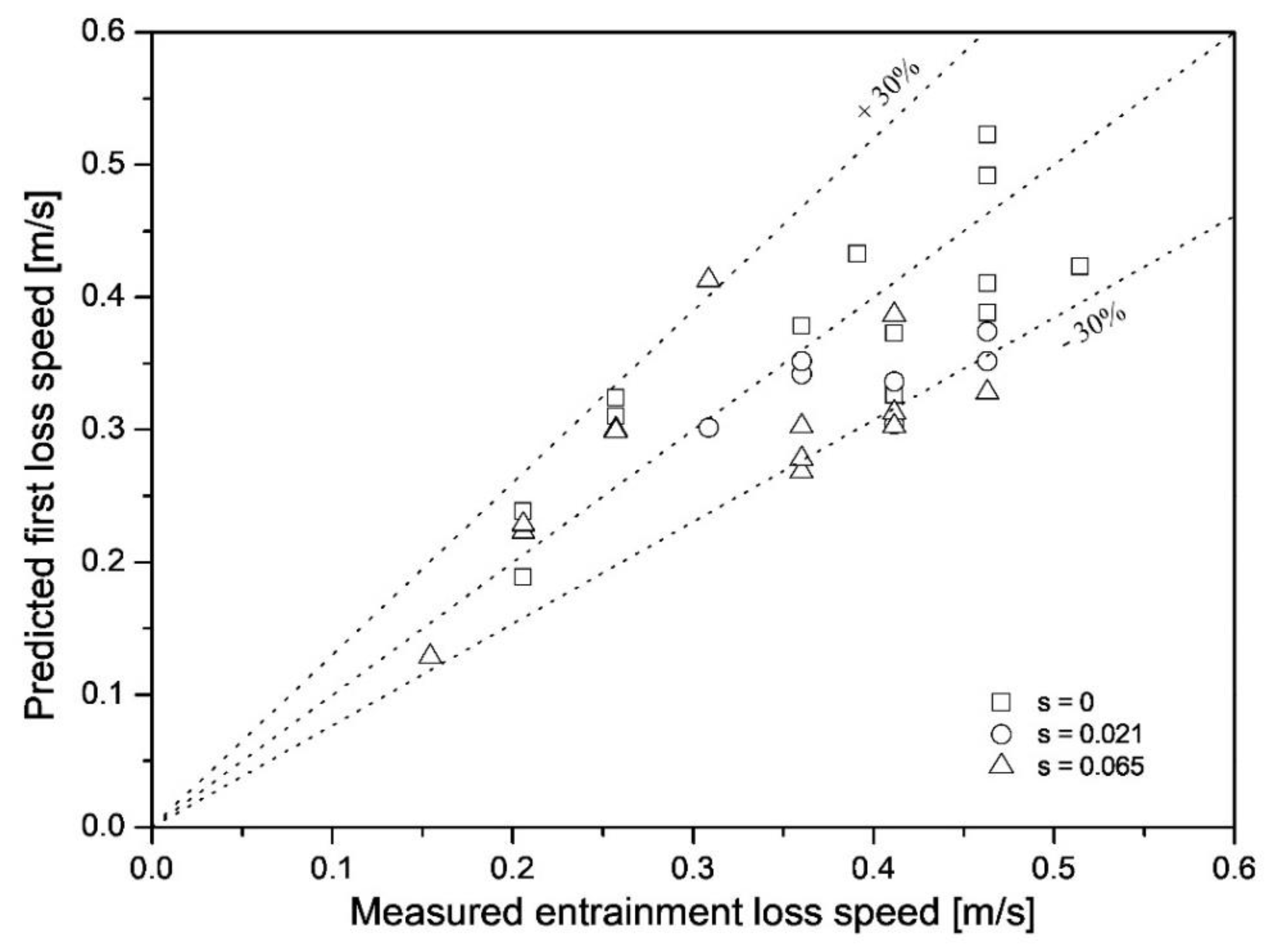
2.2.1. First Loss Speed
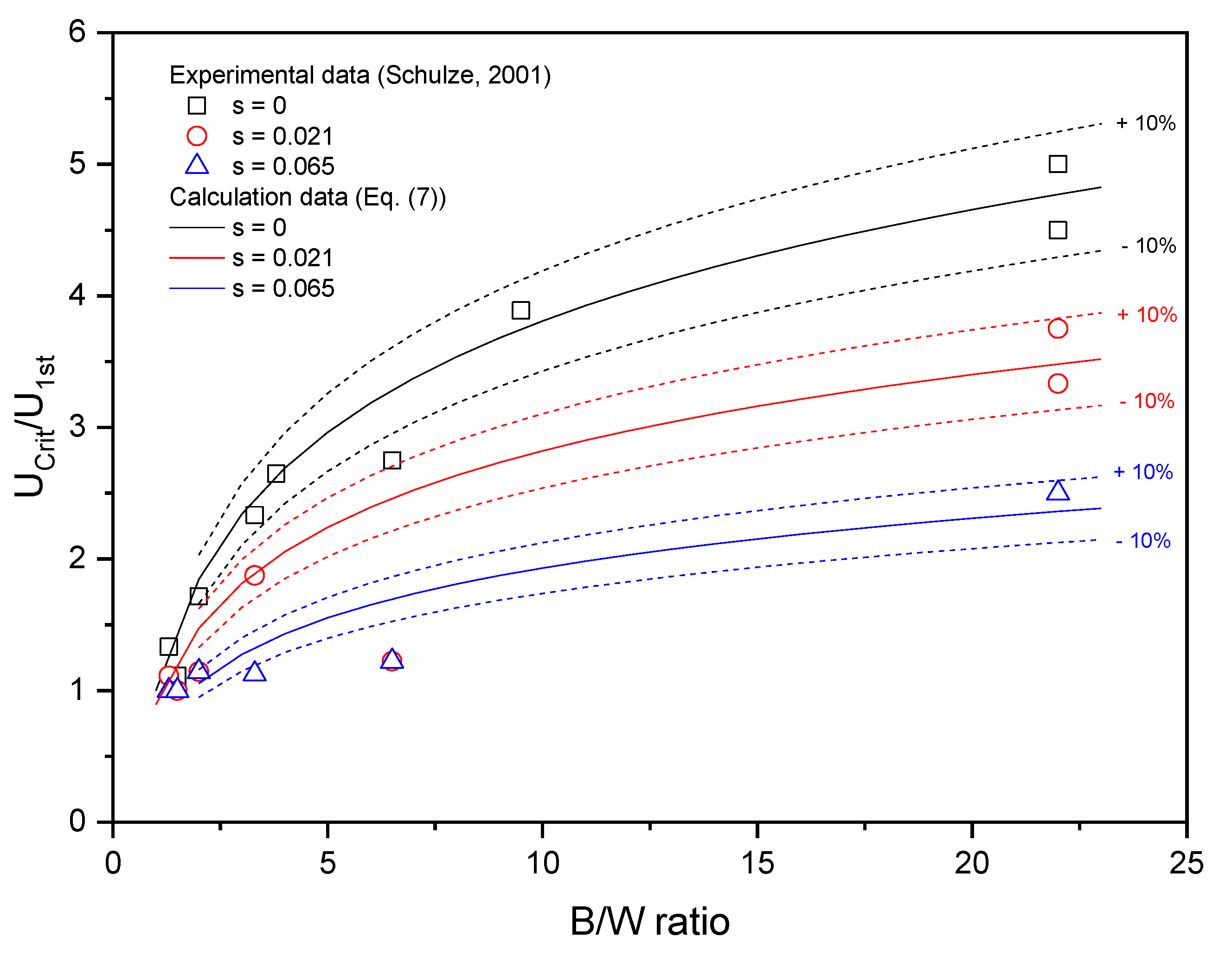
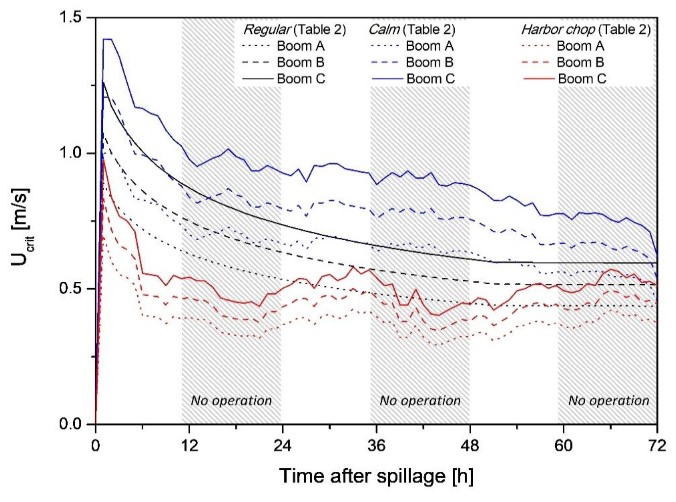
2.2.2. Critical Loss Speed
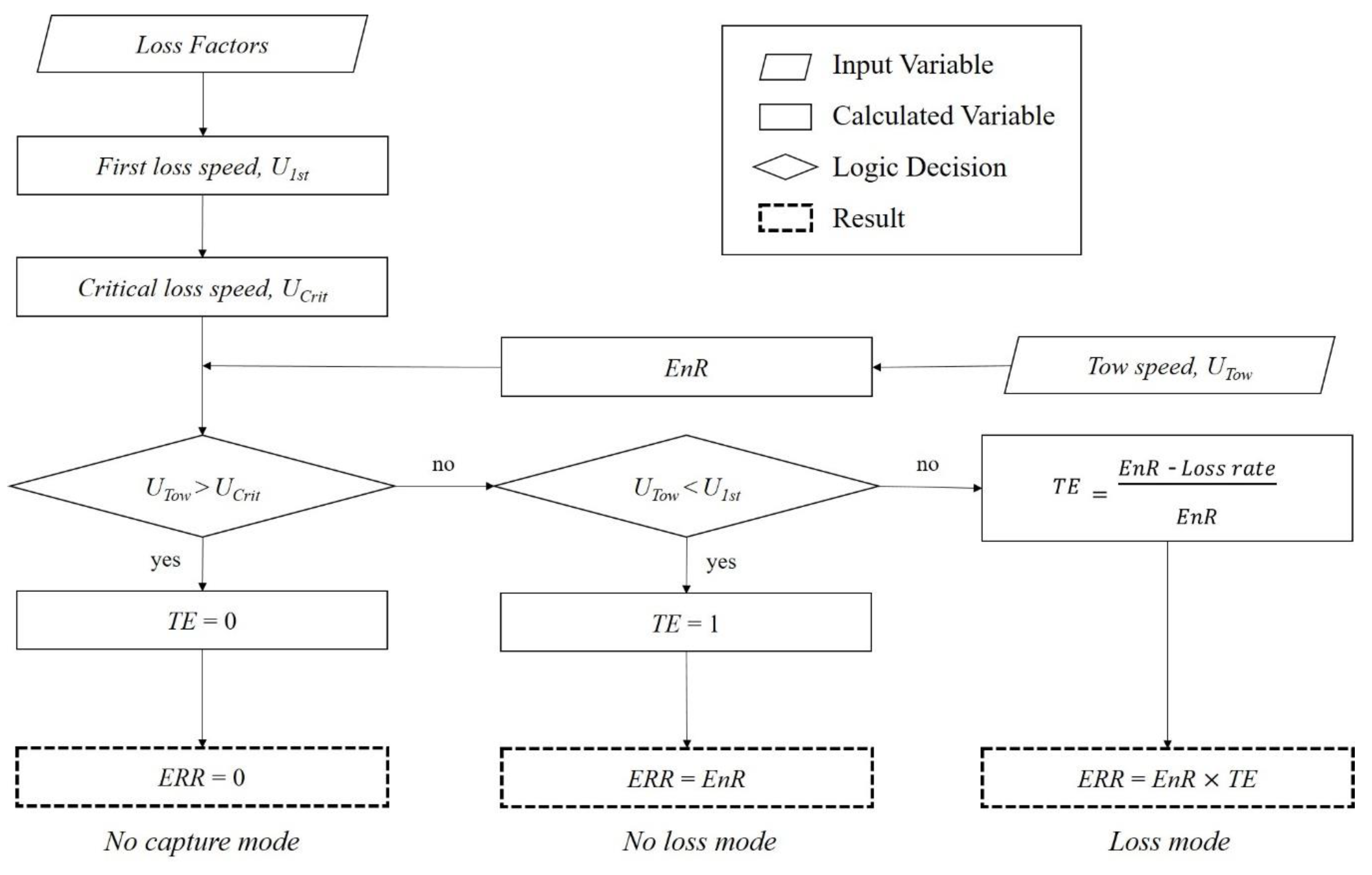
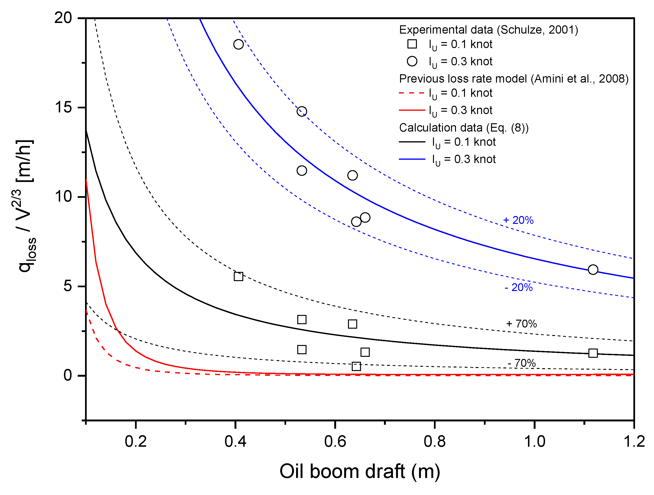
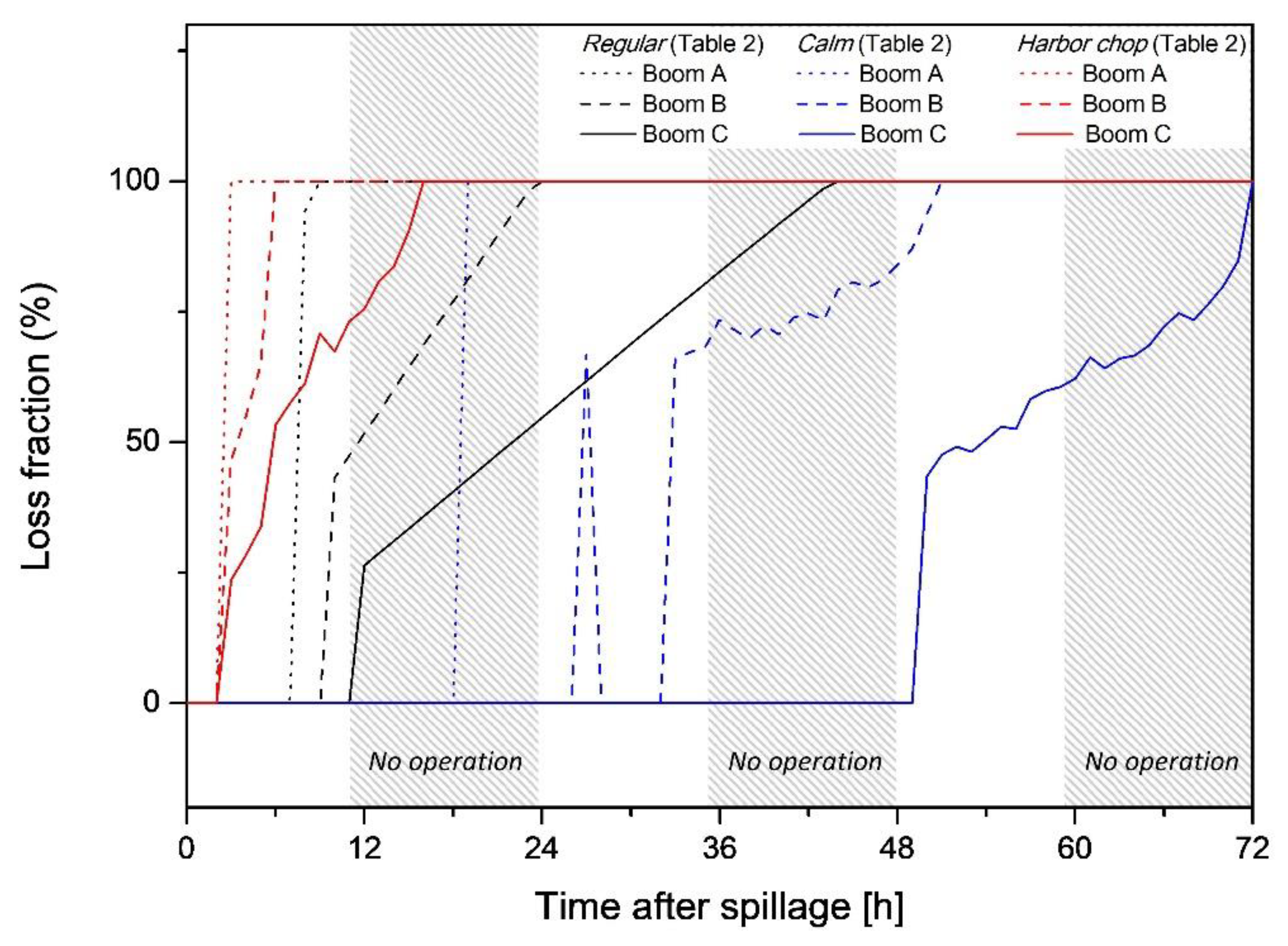
2.2.3. Loss Rate
3. Results of the Case Study
3.1. Spill Scenario of the Case Study Calculation
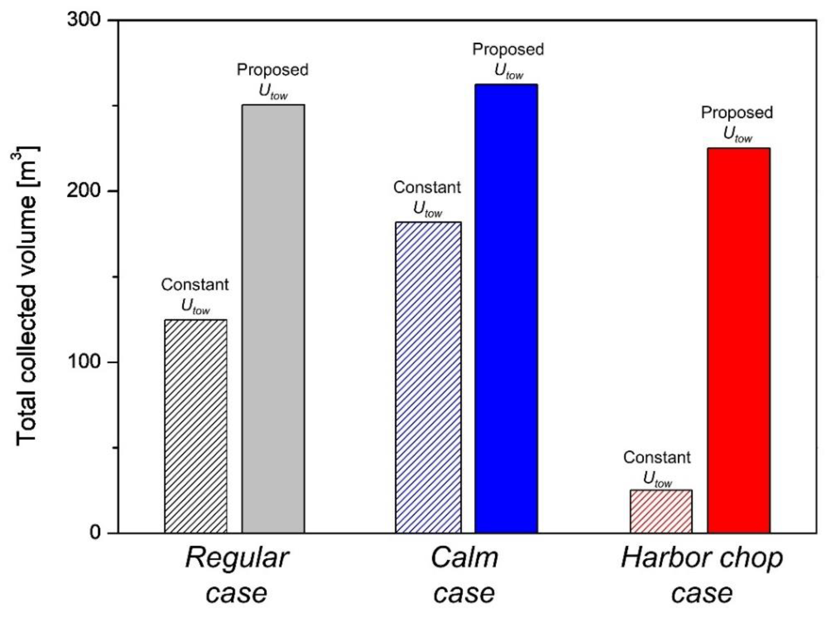
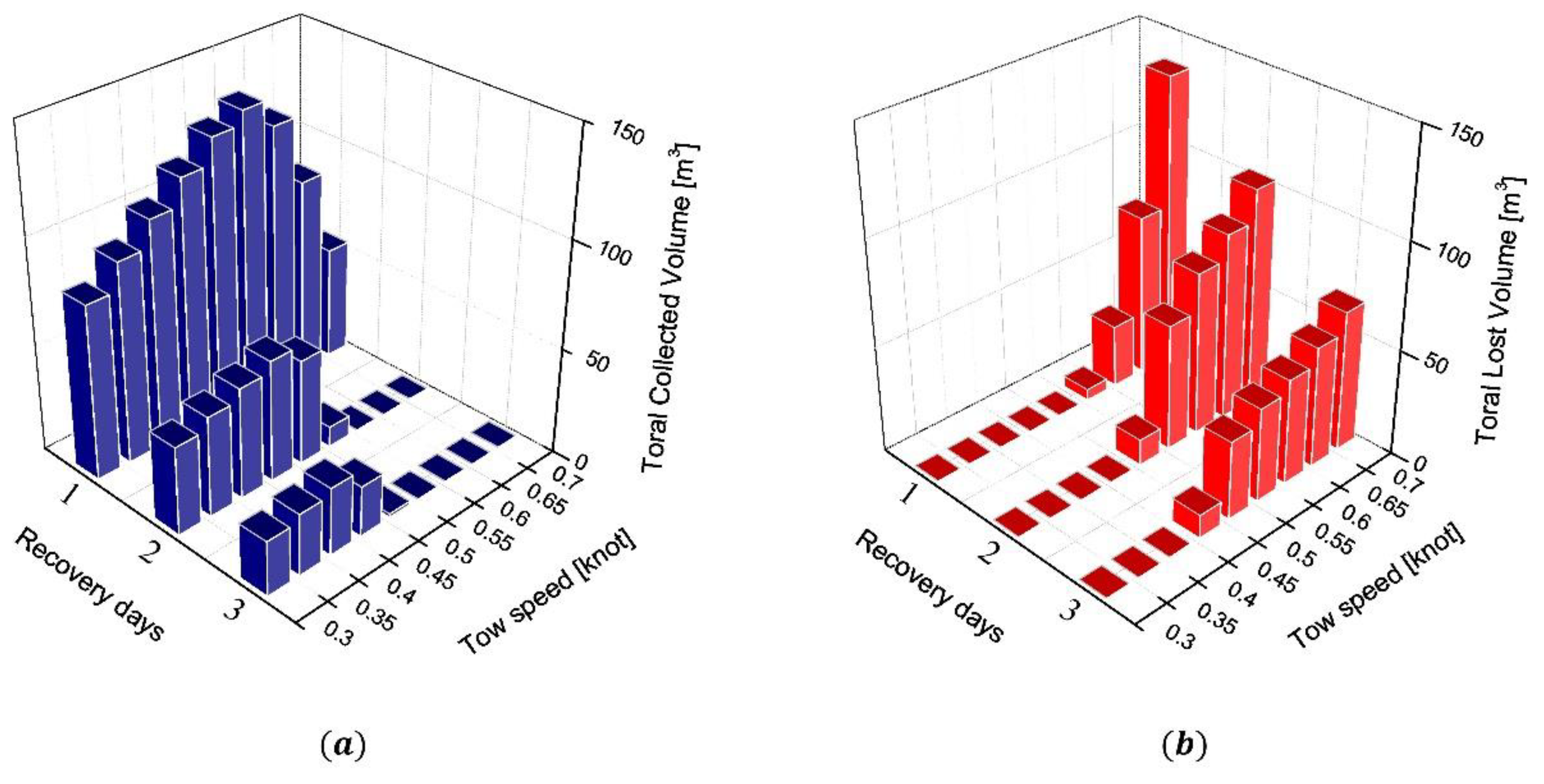
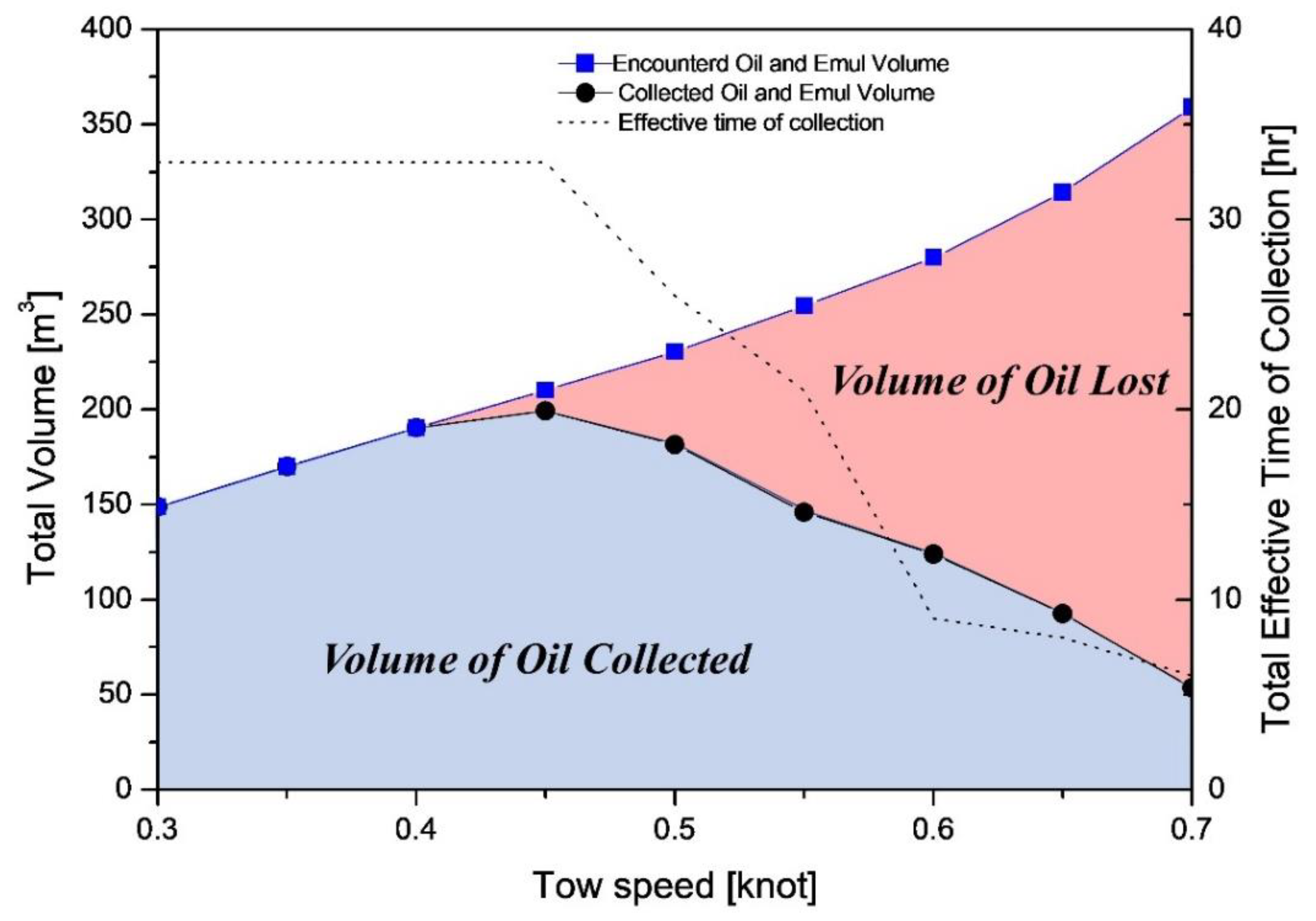
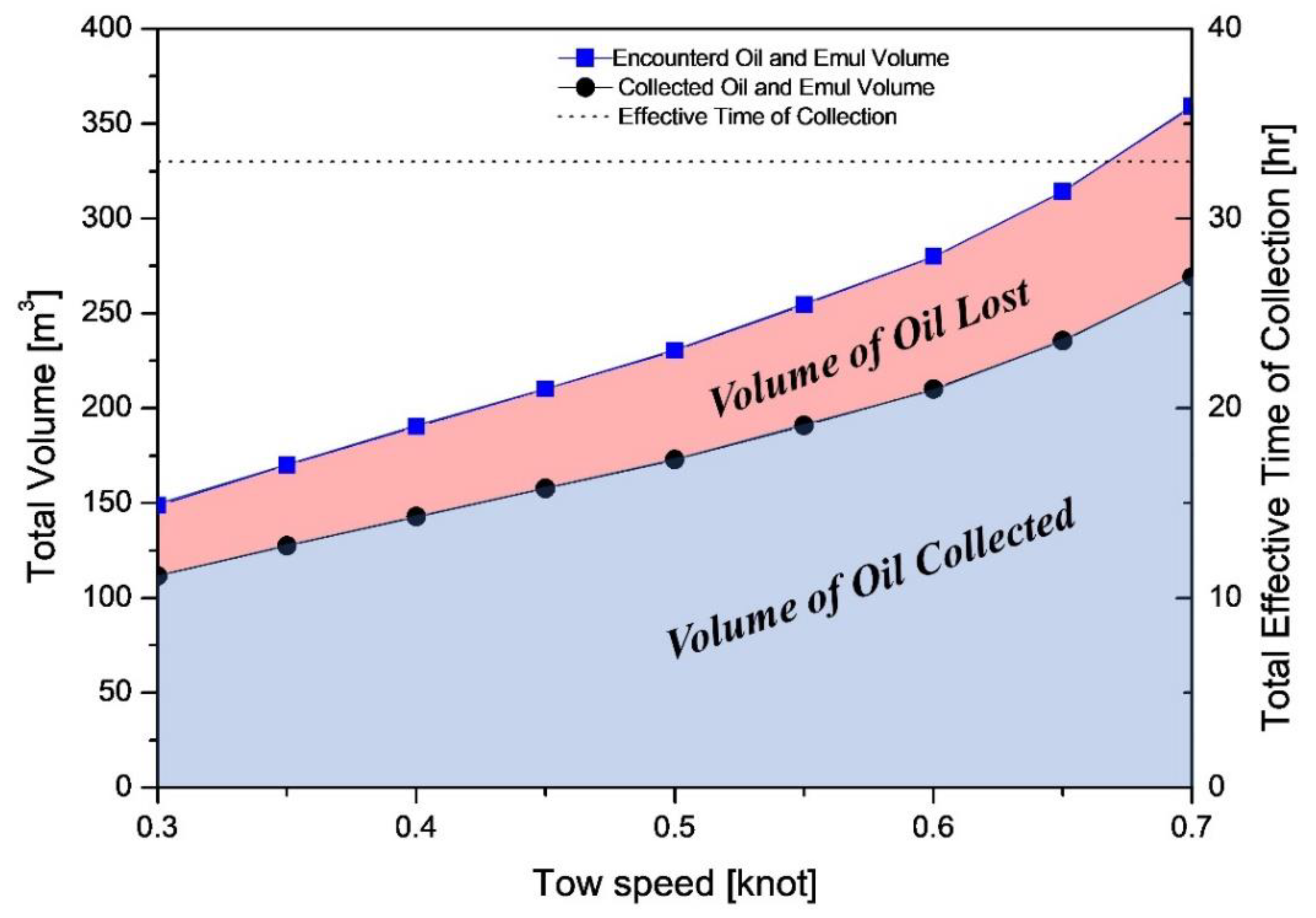
3.2. Results for Tow Speed Adjustment
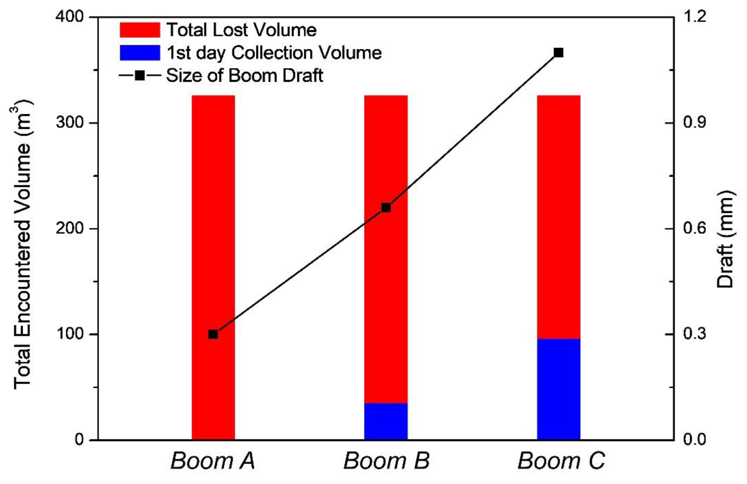
3.3. Results for Equipment Adjustment
4. Discussion
5. Conclusions
Author Contributions
Funding
Conflicts of Interest
References
- Smith, L.C.; Smith, M.; Ashcroft, P. Analysis of environmental and economic damages from British Petroleum’s Deepwater Horizon oil spill. Albany Law Rev. 2011, 74, 563–585. [Google Scholar] [CrossRef][Green Version]
- Carmo, J.S.; Pinho, J.L.; Vieira, J. Oil spills in coastal zones: Environmental impacts and practical mitigating solutions. In IMAM—Maritime Transportation and Exploitation of Ocean and Coastal Resources; BALKEMA: Amsterdam, The Netherlands, 2005; Volume 2, pp. 1689–1696. [Google Scholar]
- Castro, A.; Iglesias, G.; Carballo, R.; Fraguela, J.A. Floating boom performance under waves and currents. J. Hazard. Mater. 2010, 174, 226–235. [Google Scholar] [CrossRef] [PubMed]
- Nordvik, A.B. The technology windows-of-opportunity for marine oil spill response as related to oil weathering and operations. Spill Sci. Technol. Bull. 1995, 2, 17–46. [Google Scholar] [CrossRef]
- Ventikos, N. A high-level synthesis of oil spill response equipment and countermeasures. J. Hazard. Mater. 2004, 107, 51–58. [Google Scholar] [CrossRef] [PubMed]
- Gregory, C.L.; Allen, A.A.; Dale, D.H. Assessment of potential oil spill recovery capabilities. Int. Oil Spill Conf. Proc. 1999, 1999, 527–534. [Google Scholar] [CrossRef]
- Pinho, J.; do Carmo, J.A.; Vieira, J. Mathematical modelling of oil spills in the Atlantic Iberian coastal waters. WIT Trans. Ecol. Environ. 2004, 68, 11. [Google Scholar]
- Fingas, M.; Brown, C.E. A review of oil spill remote sensing. Sensors 2018, 18, 91. [Google Scholar] [CrossRef]
- ExxonMobil Oil Spill Response Field Manual 2014. Available online: https://corporate.exxonmobil.com/-/media/Global/Files/risk-management-and-safety/Oil-Spill-Response-Field-Manual_2014.pdf (accessed on 13 December 2019).
- Aukett, L. The Use of Geographical Information System (GIS) in Oil Spill Preparedness and Response; Society of Petroleum Engineers: Perth, Australia, 2012. [Google Scholar]
- Fingas, M. Oil Spill Science and Technology, 1st ed.; Gulf Professional Publishing: Houston, TX, USA, 2010; ISBN 978-1-85617-943-0. [Google Scholar]
- Fingas, M. Oil Spill Science and Technology, 2nd ed.; Gulf Professional Publishing: Houston, TX, USA, 2016; ISBN 978-0-12-809413-6. [Google Scholar]
- Spaulding, M.L. State of the art review and future directions in oil spill modeling. Mar. Pollut. Bull. 2017, 115, 7–19. [Google Scholar] [CrossRef]
- ASTM. ASTM F1780-18 Standard Guide for Estimating Oil Spill Recovery System Effectiveness; ASTM International: West Conshohocken, PA, USA, 2018. [Google Scholar]
- Allen, A.; Dale, D.; Galt, J.; Murphy, J. Effective Daily Recovery Capacity (EDRC) Project Final Report; Genwest Systems, Inc.: Edmonds, WA, USA, 2012; Available online: https://www.genwest.com/wp-content/uploads/2017/04/Genwest_EDRC-Project_Final_Report.pdf (accessed on 13 December 2019).
- Dale, D. Response Options Calculator (ROC) Users Guide; Genwest Systems, Inc.: Edmonds, WA, USA, 2011. [Google Scholar]
- BSEE ERSP Calculator User Manual 2015; Genwest Systems, Inc.: Edmonds, WA, USA, 2015.
- CFR Appendix B to Part 155-Determining and Evaluating Required Response Resources for Vessel Response Plans. Available online: https://www.law.cornell.edu/cfr/text/33/appendix-B_to_part_155 (accessed on 24 September 2019).
- Dale, D. Response Option Calculator (ROC) Technical Documentation; Genwest Systems, Inc.: Edmonds, WA, USA, 2011. [Google Scholar]
- ITOPF. Use of Booms in Oil Pollution Response (Technical Information Paper No. 3). 2011. Available online: https://www.itopf.org/knowledge-resources/documents-guides/document/tip-03-use-of-booms-in-oil-pollution-response/ (accessed on 13 December 2019).
- Schulze, R. Oil Spill Response Performance Review of Booms; ASTM International: West Conshohocken, PA, USA, 1988. [Google Scholar]
- Berry, A.; Dabrowski, T.; Lyons, K. The oil spill model OILTRANS and its application to the Celtic Sea. Mar. Pollut. Bull. 2012, 64, 2489–2501. [Google Scholar] [CrossRef]
- Fay, J.A. Physical Processes in the Spread of Oil on a Water Surface; American Petroleum Institute: New York, NY, USA, 1971; Volume 1971, pp. 463–467. [Google Scholar]
- Galt, J.A.; Overstreet, R. Development of Spreading Algorithms for the ROC; Response Options Calculator: Edmonds, WA, USA, 2009. [Google Scholar]
- Lehr, W.; Jones, R.; Evans, M.; Simecek-Beatty, D.; Overstreet, R. Revisions of the ADIOS oil spill model. Environ. Model. Softw. 2002, 17, 189–197. [Google Scholar] [CrossRef]
- ASTM. ASTM F631–15-Standard Guide for Collecting Skimmer Performance Data in Controlled Environments; American Society for Testing and Materials West Conshohocken: West Conshohocken, PA, USA, 2015. [Google Scholar]
- Fay, J.A. The spread of oil slicks on a calm sea. In Oil on the Sea; Springer: Berlin/Heidelberg, Germany, 1969; pp. 53–63. [Google Scholar]
- Mackay, D.; Matsugu, R.S. Evaporation rates of liquid hydrocarbon spills on land and water. Can. J. Chem. Eng. 1973, 51, 434–439. [Google Scholar] [CrossRef]
- Delvigne, G.A.L.; Sweeney, C. Natural dispersion of oil. Oil Chem. Pollut. 1988, 4, 281–310. [Google Scholar] [CrossRef]
- Eley, D.; Hey, M.; Symonds, J. Emulsions of water in asphaltene-containing oils 1. Droplet size distribution and emulsification rates. Colloids Surf. 1988, 32, 87–101. [Google Scholar] [CrossRef]
- ASTM. ASTM F2084 Standard Guide for Collecting Containment Boom Performance Data in Controlled Environments; American Society for Testing and Materials West Conshohocken: West Conshohocken, PA, USA, 2012. [Google Scholar]
- Amini, A.; Schleiss, A. Contractile Floating Barriers for Confinement and Recuperation of Oil Slicks; EPFL-LCH: Lausanne, Swiss, 2007. [Google Scholar]
- ASTM. ASTM F2683-11(2017) Standard Guide for Selection of Booms for Oil-Spill Response; ASTM International: West Conshohocken, PA, USA, 2017. [Google Scholar]
- ASTM. ASTM F625/F625M-94(2017) Standard Practice for Classifying Water Bodies for Spill Control Systems; ASTM International: West Conshohocken, PA, USA, 2017. [Google Scholar]
- Brown, H.M.; Goodman, R.H.; An, C.-F.; Bittner, J. Boom failure mechanisms: Comparison of channel experiments with computer modelling results. Spill Sci. Technol. Bull. 1996, 3, 217–220. [Google Scholar] [CrossRef]
- Goodman, R.H.; Brown, H.M.; An, C.-F.; Rowe, R.D. Dynamic modelling of oil boom failure using computational fluid dynamics. Spill Sci. Technol. Bull. 1996, 3, 213–216. [Google Scholar] [CrossRef]
- Oebius, H.U. Physical properties and processes that influence the clean up of oil spills in the marine environment. Spill Sci. Technol. Bull. 1999, 5, 177–289. [Google Scholar] [CrossRef]
- Wicks, M. Fluid Dynamics of Floating Oil Containment by Mechanical Barriers in The Presence of Water Currents. In Proceedings of the International Oil Spill Conference Proceedings, Houston, TX, USA, December 1969; Volume 1969, pp. 55–106. [Google Scholar]
- Agrawal, R.K.; Hale, L.A. A New Criterion for Predicting Headwave Instability of an Oil Slick Retained by a Barrier. In Proceedings of the Offshore Technology Conference, Houston, TX, USA, 6–8 May 1974. [Google Scholar]
- Leibovich, S. Oil slick instability and the entrainment failure of oil containment booms. J. Fluids Eng. 1976, 98, 98–103. [Google Scholar] [CrossRef]
- Milgram, J.S.; Van Houten, R.S. Mechanics of a Restrained Layer of Floating Oil above a Water Current. J. Hydronautics 1978, 12, 93–108. [Google Scholar] [CrossRef]
- Lee, C.M.; Kang, K.H. Prediction of oil boom performance in currents and waves. Spill Sci. Technol. Bull. 1997, 4, 257–266. [Google Scholar] [CrossRef]
- Amini, A.; Schleiss, A.J. Behavior of rigid and flexible oil barriers in the presence of waves. Appl. Ocean Res. 2009, 31, 186–196. [Google Scholar] [CrossRef]
- Potter, S. The Effect of Buoyancy-to-weight Ratio in Oil Spill Containment Boom Performance; S.L. Ross Environmental Research Limited: Ottawa, ON, Canada, 2003. [Google Scholar]
- Amini, A.; Bollaert, E.; Boillat, J.-L.; Schleiss, A.J. Dynamics of low-viscosity oils retained by rigid and flexible barriers. Ocean Eng. 2008, 35, 1479–1491. [Google Scholar] [CrossRef]
- Fannelop, T.K. Loss rates and operational limits for booms used as oil barriers. Appl. Ocean Res. 1983, 5, 80–92. [Google Scholar] [CrossRef]
- Lindenmuth, W.T.; Miller, E.R.J.; Hsu, C.C. Studies of Oil Retention Boom Hydrodynamics; Hydronautics, Inc.: Laurel, MD, USA, 1970. [Google Scholar]
- Potter, S. World Catalog of Oil Spill Response Products; S.L. Ross Environmental Research Limited: Ottawa, ON, Canada, 2004. [Google Scholar]
- Korea Hydrographic and Oceanographic Agency Oceanographic Observation Portal. Available online: http://www.khoa.go.kr/kcom/cnt/selectContentsPage.do?cntId=31000000 (accessed on 24 September 2019).


| Category | Variables | Value | ||
|---|---|---|---|---|
| Simulation time | Calculation time | 72 h | ||
| Recovery time | 33 h | |||
| Calculation unit time | 1 h | |||
| Oil | Initial spill volume | 500 m3 (Batch spill) | ||
| Oil type | Iranian heavy (API 30) | |||
| Recovery system | Skimmer model (Nameplate capacity) | Lamor LWS (140 m3/h) | ||
| Boom type | Boom A | Boom B | Boom C | |
| Boom model | ACME CONTRACTOR BOOM (Curtain, internal foam) | LAMOR HDB 1300 (Curtain, pressure inflatable) | DESMI RO-BOOM 2000 (Curtain, pressure inflatable) | |
| Draft | 0.3 m | 0.66 m | 1.1 m | |
| B/W ratio | 6.2 | 9 | 13 | |
| Operating condition | Swath | 100 m (boom length/3) | ||
| Tow speed | 0.5 knot (0.257 m/s) | |||
| Case | Environmental Condition | Wave Steepness (period) | Wind Speed [m/s] (period) |
|---|---|---|---|
| Case 1 | Regular (average) | 0.01 (constant) | 5 m/s (constant) |
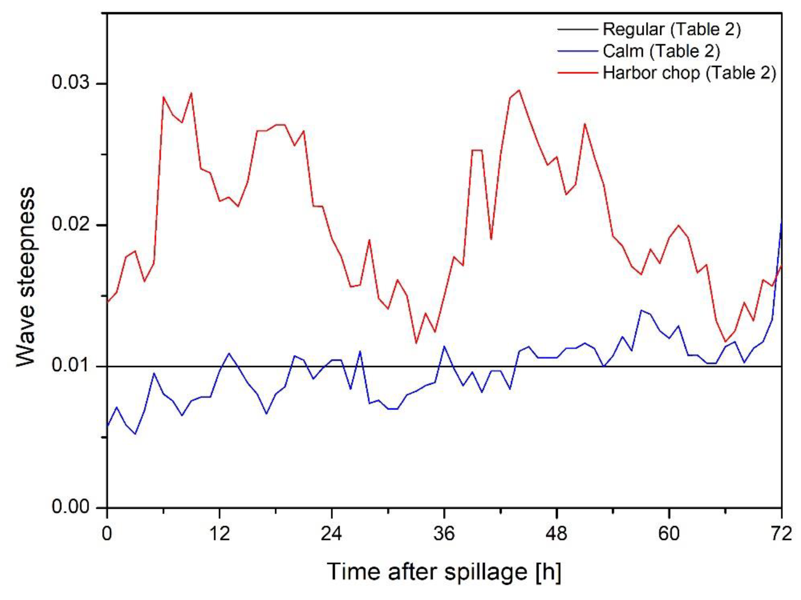
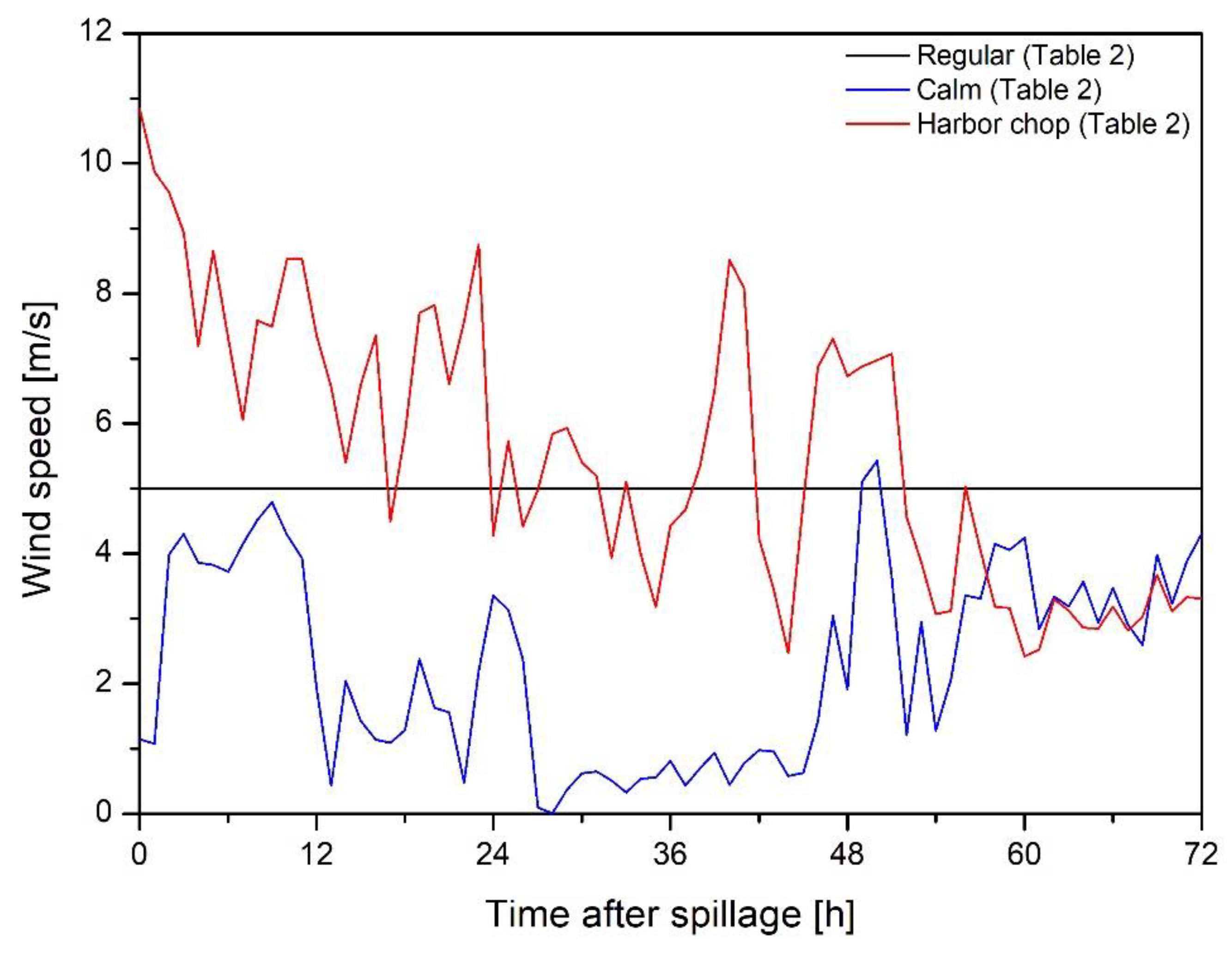
| Case 2 | Calm | Figure 7 (2017.07.21.07–2017.07.24.06) | Figure 8 (2017.07.21.07–2017.07.24.06) |
| Case 3 | Harbor chop | Figure 7 (2017.01.14.07–2017.01.17.06) | Figure 8 (2017.01.14.07–2017.01.17.06) |
© 2019 by the authors. Licensee MDPI, Basel, Switzerland. This article is an open access article distributed under the terms and conditions of the Creative Commons Attribution (CC BY) license (http://creativecommons.org/licenses/by/4.0/).
Share and Cite
Kim, H.; Choe, Y.; Huh, C. Estimation of a Mechanical Recovery System’s Oil Recovery Capacity by Considering Boom Loss. J. Mar. Sci. Eng. 2019, 7, 458. https://doi.org/10.3390/jmse7120458
Kim H, Choe Y, Huh C. Estimation of a Mechanical Recovery System’s Oil Recovery Capacity by Considering Boom Loss. Journal of Marine Science and Engineering. 2019; 7(12):458. https://doi.org/10.3390/jmse7120458
Chicago/Turabian StyleKim, Hyeonuk, Yunseon Choe, and Cheol Huh. 2019. "Estimation of a Mechanical Recovery System’s Oil Recovery Capacity by Considering Boom Loss" Journal of Marine Science and Engineering 7, no. 12: 458. https://doi.org/10.3390/jmse7120458
APA StyleKim, H., Choe, Y., & Huh, C. (2019). Estimation of a Mechanical Recovery System’s Oil Recovery Capacity by Considering Boom Loss. Journal of Marine Science and Engineering, 7(12), 458. https://doi.org/10.3390/jmse7120458