The Numerical Prediction and Analysis of Propeller Cavitation Benchmark Tests of YUPENG Ship Model

Abstract

The numerical simulation of propeller cavitation benchmark tests of YUPENG ship model is studied based on OpenFOAM, an open-source CFD (Computational Fluid Dynamics) platform, and the benchmark tests are introduced as well. The propeller cavitation shape and the hull pressure fluctuation are measured and predicted, respectively. The uncertainty in hull pressure fluctuation measurement is also analyzed, and the analysis showed the uncertainty is below 10%. The cavitation shape and the hull pressure fluctuation predicted show quite good agreement with the observations and measured data, and the influences of the grid resolutions on the unsteady propeller cavitation and the hull pressure fluctuation are investigated as well. The monotonic convergence achieved and the quite small grid uncertainty illustrate the reliability of the numerical simulation methods.

1. Introduction

Propeller cavitation is one important aspect of hydrodynamic performance for marine propellers, and recently it has been studied based on viscous numerical simulation methods, especially the viscous RANS (Reynolds Average Navier-Stokes) approach, and more and more research articles have been published. Salvatore [1] has studied the cavitation on the standard INSEAN E779A propeller and compared the cavitation predictions using several different solvers and cavitation models. The discrepancies in cavity extent are observed in the comparative analysis. Li [2] has also predicted the cavitating flows around the INSEAN E779A propeller in non-uniform wake, using a RANS approach and Zwart cavitation model based on commercial FLUENT. The numerical results show that the key features predicted, such as the attached cavity and the collapse of the main cavity, resemble well with the experiment observations. Paik [3] has conducted the simulations of cavitating flows for a marine propeller based on FLUENT and Schnerr-Sauer cavitation model. The simulation results show reliable performance on the prediction of cavitation shape and hull pressure fluctuation. Vaz [4] has compared more cavitation and pressure pulse predictions between different solvers and cavitation models, the results indicate that the pressure fluctuations predicted by half the participants are in reasonable agreement with measurements, but the remaining calculations predict pressure levels a factor of four or five too high. Fujiyama [5] has analyzed the unsteady cavitating flow of HSP-II and CP-II propeller at behind-hull condition both in model and full scale, using commercial software SC/Tetra v13. The results show that the unsteady propeller cavitation phenomena can be captured in the numerical calculation. Long [6] has researched the propeller cavitating flow behind the hull, analyzed the vorticity distribution and particle tracks as well, using commercial software CFX and Zwart cavitation model. The cavitation patterns predicted resemble well with the experimental observations, with some over-prediction of the cavitation area. Yilmaz [7] has investigated the hull–propeller–rudder interaction in the presence of tip vortex cavitation, using commercial software STAR-CCM+ and Schnerr-Sauer cavitation model with LES (Large eddy simulation) method. The investigation results demonstrate some capability of STAR-CCM+ for investigation in the presence of tip vortex cavitation.

In addition to commercial CFD software, an open-source CFD platform, OpenFOAM has been increasingly used to conduct the numerical simulation of propeller cavitating flows. Abolfazl [8] has performed the numerical prediction of the PPTC (Potsdam Propeller Test Case) propeller cavitation size in oblique wake based on ILES (Implicit Large Eddy Simulation) approach and Schnerr–Sauer cavitation model, using OpenFOAM. The simulation results show over-prediction of the propeller cavitation extent. Bensow [9] has carried out a prediction of a marine propeller behind a chemical tanker with ILES approach and Kunz cavitation model, based on OpenFOAM. The prediction of cavity area shows good agreement with the experiments. Zheng [10,11] has simulated the unsteady propeller cavitating flows in the stern of a ship using unsteady RANS approach, based on OpenFOAM. The predicted cavitation shape change shows quite good agreement with the experimental observation.

The present study aims to research the influence of the grid resolutions on the unsteady propeller cavitation and the induced hull pressure fluctuation behind the YUPENG benchmark ship model, which will illustrate the reliability of the numerical simulation methods.

2. Mathematic Base

2.1. Governing Equations

The unsteady RANS method is applied in the present study for the significantly lower computational resources needed compared with LES.

The time-averaged continuity equation and momentum equation are shown in Equations (1) and (2), respectively.

$$\frac{\partial \rho }{\partial t}+\nabla \left(\rho U\right)=0$$

(1)

$$\frac{\partial \rho U}{\partial t}+U·\nabla \left(\rho U\right)=\nabla \left(\left(\mu +{\mu }_t\right)\nabla U\right)-\nabla p-F_S$$

(2)

where U is the averaged velocity vector, p is the mean pressure. $\rho$ is the fluid density, μ is the dynamic viscosity, and μ_t is the turbulent viscosity. F_S is the surface tension force which takes place only at the free surfaces. The turbulent viscosity μ_t is modeled by the SST kw [12] turbulence model combined with wall functions.

According to the VOF (Volume of Fluid) method, the physical properties of the cavitating flows are scaled by the volume fraction of water γ, with γ = 1 corresponding to pure water, γ = 0 corresponding to pure vapor, 0 < γ < 1 corresponding to the interface between water and vapor.

Thus, the density and dynamic viscosity of the cavitating flows are scaled as follows. The subscripts w and v represent water and vapor, respectively.

$$\rho =\gamma {\rho }_w+\left(1-\gamma \right){\rho }_v$$

(3)

$$\rho =\gamma {\mu }_w+\left(1-\gamma \right){\mu }_v$$

(4)

The transport equation of the volume fraction of water γ can be written as follows.

$$\frac{D_{\gamma }}{D_t}=\frac{\partial \gamma }{\partial t}+\nabla \left(\gamma U\right)=\frac{\dot{m}}{{\rho }_w}$$

(5)

Here, the mass transfer rate, $\dot{m}$, between water and vapor is to be modeled by cavitation model.

Combining with Equations (3) and (5), the mass transport, Equation (1) can be re-written as follows.

$$\nabla ·U=\dot{m}\left(\frac{1}{{\rho }_w}-\frac{1}{{\rho }_v}\right)$$

(6)

It suggests that the mass transport rate, $\dot{m}$, between water and vapor participates in the coupled solving procedure of pressure and velocity. During the simulations of cavitating flows, $\dot{m}$ is calculated in the PISO (Pressure Implicit with Splitting of Operators) [13] loop at first, then the transport equation of the vapor volume fraction is solved and the standard PISO procedure is progressed.

2.2. Cavitation Model

Cavitation is a complex hydrodynamic phenomenon and is generally simplified as the transition of water into vapor in the region where the local pressure is lower than the water saturation pressure during the numerical simulation. The transition is caused by the small gas nuclei in the water. In order to mimic the phase change between water and vapor, the Schnerr–Sauer cavitation model is adopted.

$$\dot{m}=sign\left({\rho }_v-\rho \right) \frac{n_0}{1+n_0\frac{4}{3}\pi R^3}4\pi R^2\sqrt{\frac{2}{3}\frac{|{\rho }_v-\rho |}{{\rho }_w}}$$

(7)

Here, n₀ is the number of micro gas nuclei per water volume, and R is the initial radius of micro gas nuclei. The values of n₀ and R are default, e.g., n₀ = 1.6 × 10¹³, R = 2.0 × 10⁻⁶. Schnerr–Sauer cavitation model can be deduced based on Rayleigh–Plesset equation describing the bubble dynamics.

3. Calculation Modeling

3.1. Calculation Object

The investigated object is the YUPENG benchmark ship, which is a 30,000 DWT bulk carrier driven by a fixed-pitch four-bladed propeller. The benchmark propeller cavitation model test including cavitation observation and pressure fluctuation measurement is conducted in the Large Cavitation Channel (LCC) of the China Ship Scientific Research Center (CSSRC). The principal parameters of ship and propeller model are shown in Table 1 and Table 2, respectively. The hull, rudder, and propeller are visualized in Figure 1.

Table 1. Principal parameters of YUPENG model.

LPP (m)	7.0522
Design draught (m)	0.3843
Shaft height (m)	0.1343

Table 2. Principal parameters of YUPENG propeller model.

Diameter (m)	0.250	Area ratio	0.48
No. of blades	4	P/D (0.7R)	0.80
Hub ratio	0.147	Skew angle (°)	24.5

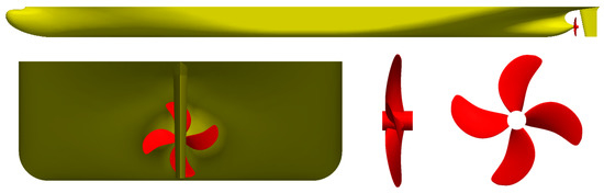
Figure 1. YUPENG ship and propeller geometry model.

The benchmark test setup inside the LCC is shown in Figure 2. The initial rotating angle, φ, is defined as 0° at twelve o’clock, and the propeller has been assembled and oriented at the initial position.

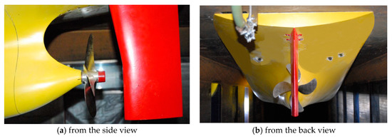
Figure 2. The benchmark test set.

3.2. Computational Domain and Boundary Condition

The whole computational domain is a box of 7L_pp × 4L_pp × 2L_pp. The boundary conditions on the front, bottom, and sides are velocity inlet, and the boundary condition on the top is symmetry, the boundary condition on the back is pressure outlet, as shown in Figure 3.

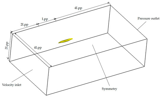
Figure 3. The computational domain and boundary conditions.

The whole computational domain consists of two sub-domains, the ship sub-domain and the propeller sub-domain. The ship sub-domain is a static region which includes the boundary of the inlet, outlet, hull, and rudder. The propeller sub-domain is a rotating region surrounding the propeller. All the grids of the two sub-domains consists of unstructured hexahedral cells of high quality. For more accurate prediction of the flow detail, several boundary layer cells are inserted near wall surfaces. The overview of the hull, rudder, and propeller surface is shown in Figure 4. The arbitrary mesh interface (AMI) method is applied to interpolate between the non-conforming interfaces of the two sub-domains.

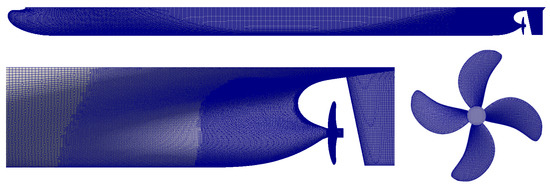
Figure 4. The overview of the hull, rudder, and propeller surface grid.

The velocity inlet condition is set to be a fixed value of velocity, U, at the inlet boundary, U = 5.481 m/s, and the turbulence intensity at the inflow is 0.1%. The pressure outlet condition is set to be a fixed value of pressure, which is constant based on the cavitation number, σ_n(0.8R), at the outlet boundary. The no-slip wall condition is set at the hull, rudder, and propeller boundary.

4. Calculation Result Analysis

The benchmark test conditions numerically predicted in the present study are summarized in Table 3.

Table 3. The test conditions

Parameters	Design Draft
n (rps)	28
σn(0.8R)	0.3154
KT	0.1371

n—rotating speed of the propeller, σ_n(0.8R)—cavitation number basing the rotating speed, K_T—the thrust coefficient of the propeller.

The formulae are as follows.

$${\sigma }_{n\left(0.8R\right)}=\frac{p-p_v}{0.5\rho {\left(0.8\pi nD\right)}^2}$$

(8)

$$K_T=\frac{T}{\rho n^2{D}^4}$$

(9)

The free surface is neglected, and the effect of the stern wave on pressure is not taken into account either in the experiment or in the numerical calculation, because the stern wave height of the low-speed vessel (Fr < 0.2) is generally less than 0.5 m at full scale, which will be negligible at model scale in the experiment.

For the computational convergence, the numerical simulation of the steady full wet flow is conducted to obtain a quasi-stable flow field using the multiple reference frame (MRF) method, then the unsteady calculation is started to simulate the propeller rotation using sliding mesh method, and the cavitation calculation is started to predict the propeller cavitating flows by activating the cavitation model, finally. Ten revolutions are simulated after the sliding mesh method is started, and 1° per time step is used both in unsteady and cavitation calculations.

4.1. Grid Independence

In order to investigate the grid independency, three grid sizes were chosen, as shown in Table 4 and Figure 5. All the ship and propeller regions consist of unstructured hexahedral cells with the same grid topology, generated by HEXPRESS, and the grid refinement ratio is $\sqrt{2}$.

Table 4. The three systematic refined grids.

Number of Cells	Grid 1	Grid 2	Grid 3
Ship region	16,136,913	6,797,553	2,804,256
Propeller region	3,019,932	1,096,318	523,144
Total	19,156,845	7,893,871	3,327,400

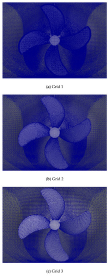
Figure 5. The surface mesh of ship stern and propeller.

There are 120 CPU cores used in the numerical simulation, and the time cost for the unsteady cavitation prediction in the three refined grids is recorded in Table 5.

Table 5. The time cost for the unsteady cavitation simulation.

Time Cost	Grid 1	Grid 2	Grid 3
T (hours)	12.04	3.84	1.30

The variation of the thrust coefficient K_T over the last full propeller revolution is shown in Figure 6, and the results show that it is obviously periodic.

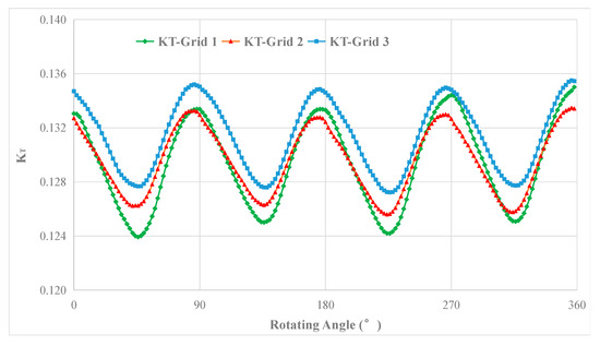
Figure 6. The variation of the thrust coefficient K_T over the last full propeller revolution.

The influence of grid resolution on K_T is assessed in Table 6. Based on the procedure recommended by ITTC [14]; the grid uncertainty, U_G; the corrected benchmark solution, S_C; and the convergence ratio, R_G, are also evaluated using the grid convergence index (GCI) approach proposed by Roache [15].

Table 6. The difference between prediction and measurement of K_T; grid uncertainty, U_G; and convergence ratio, R_G.

Parameters	Grid 1	Grid 2	Grid 3	Experiment
KT	0.1293	0.1296	0.1314	0.1371
SC	0.129			-
Difference	−5.65%	−5.47%	−4.19%	-
UG	0.00024			-
UG/SC	0.186%			-
RG	0.167			-

S_c—corrected benchmark solution.

In Table 6, the K_T predicted using the three grids agrees well with the measured value, and the R_G obtained shows that monotonic convergence was achieved for 0 < R_G < 1, the relative grid uncertainty, U_G/S_C, is also small, so all these predicted results illustrate the reliability of the numerical simulation methods adopted in the present study.

4.2. Cavitation Shape

The predicted cavity is represented by vapor iso-surface, and it is true that different value of γ_v used for the iso-surface can affect the cavitation area, e.g., a larger area with the lower value and a smaller area with the higher value. The two values of γ_v, 0.5 and 0.1, are used to represent the cavitation pattern in Figure 7. The results show that the dependence is limited, and the cavitation retains the main shape.

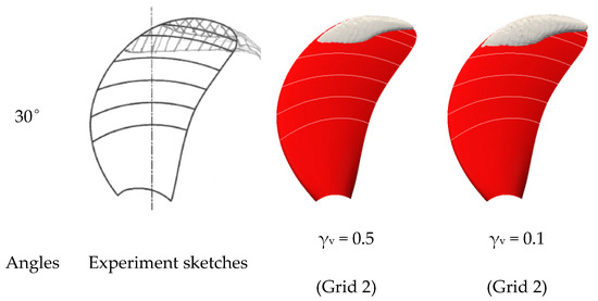
Figure 7. The predicted propeller cavitation represented by different values of vapor iso-surface.

The predicted propeller cavitation using three refined grids behind the stern is compared with benchmark test sketches at the corresponding rotating angles in Figure 8.

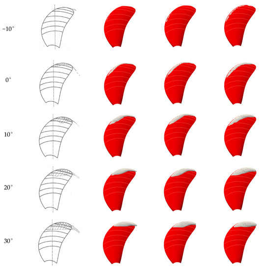
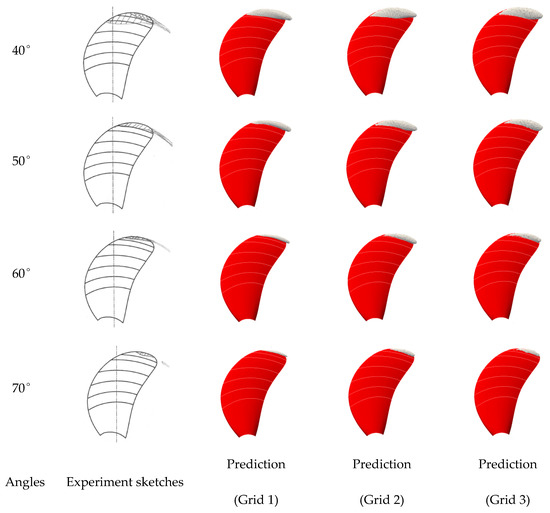
Figure 8. The predicted propeller cavitation shape compared with the benchmark test sketches.

In Figure 8, the predicted cavity using three refined grids, represented by vapor iso-surface of 0.1, shows the same dynamic behavior (e.g., the change of the propeller cavitation shape) as the benchmark test observations. The main feature, the shape change of the attached cavity along with the rotating angles, correlates well with the test sketches, e.g. the cavitation appears at about the same angle, φ ≈ −10°, and reaches the maximum size at φ ≈ 30°. Nevertheless, the tip vortex cavity cannot be predicted well on account of the insufficient grid resolution near the blade tip. In addition, the difference of the cavity predicted among the three grids is not obvious, and it implies that Grid 2 can obtain satisfactory efficiency and precision of the unsteady propeller cavitation.

4.3. Hull Pressure Fluctuation Induced by Cavitation

The hull pressure fluctuation induced by propeller cavitating flows is an important index that evaluates the propeller cavitation performance, so the monitoring points on the hull surface in the stern region are arranged as shown in Figure 9.

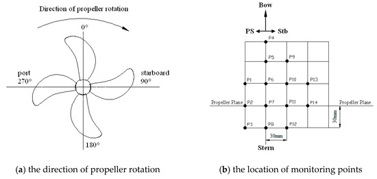
Figure 9. The arrangement of monitoring points.

The variation of the pressure at P10 over the last full propeller revolution is shown in Figure 10, and the results show it is obviously periodic as well.

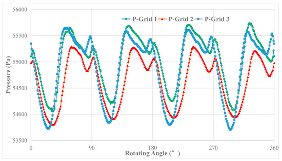
Figure 10. The variation of pressure at P10 over the last full propeller revolution.

Similar to experimental analysis, the pressure fluctuation calculated at model scale is firstly analyzed by the fast Fourier transformation (FFT) method, then converted to the one at full scale. The conversion formula is as follows.

$$K_{P_i}=\frac{\mathsf{\Delta }{P}_{im}}{{\rho }_m{n}_m^2{D}_m^2} \left(i=1,2,3\dots .\right)$$

(10)

$$\mathsf{\Delta }{P}_{is}=K_{P_i}·{\rho }_{sea}·n_s^2·D_s^2 \left(i=1,2,3\dots .\right)$$

(11)

Firstly, the hull pressure fluctuation predicted in non-cavitating condition is compared with the experiment, as shown in Figure 11. The 1BF signifies the first blade frequency component of the pressure fluctuation.

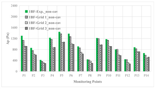
Figure 11. The 1BF (first blade frequency) component of hull pressure fluctuation predicted compared with the test data in non-cavitating condition.

It indicates that the maximum value of the 1BF component of the hull pressure fluctuation is at P5 in the non-cavitating condition, and the values decrease rapidly near the propeller in the vertical plane, such as from P1 to P3, from P5 to P8, and from P9 to P12. The results achieved with Grid 1 are much better than those of the other grids.

For the uncertainty analysis in cavitating condition, the hull pressure fluctuation measurement has been repeated three times, and the maximum value of the 1BF component of the hull pressure fluctuation is at P10 each time. The uncertainty contribution of the measurement, the combined uncertainty, and the expanded uncertainty [16] are counted in Table 7. The analysis shows that the expanded uncertainty is below 10%.

Table 7. The expanded uncertainty in measurement for the 1BF component of the hull pressure fluctuation in cavitating condition (at P10).

ΔPS	Type	Uncertainty	Remark
Propeller diameter	B	0.04%	negligible
Operating pressure	B	0.11%	negligible
Saturated vapor pressure	B	0.29%	negligible
Water density	B	0.001%	negligible
Propeller rotate speed	B	0.02%	negligible
Dynamic pressure transducer	B	3.33%	dominant
Repeat test (N = 3)	A	0.70%	minor
Combined uncertainty		3.42%	-
Expanded uncertainty		6.83%	-

The amplitudes of the 1BF component of the hull pressure fluctuation converted at full scale are compared with the benchmark test data in Figure 12. The maximum value of the 1BF component of the hull pressure fluctuation is at P10 in the cavitating condition, while it is at P5 in the non-cavitating condition. This is mainly due to the rapid change of the cavitation volume at about φ ≈ 30°, which causes the levels of the pressure pulse at P10 to be higher.

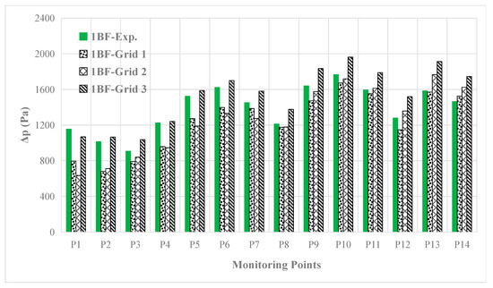
Figure 12. The 1BF component of hull pressure fluctuation predicted compared with the test data.

The predicted results obtained show quite good agreement with the benchmark test. It is found that not only the spatial laws but also the maximum value of 1BF component of the hull pressure fluctuation, which is mostly of great concern in engineering, can be predicted well. It seems that the calculated value of Grid 2 is a little closer to the test than that of Grid 1 at P10.

Moreover, the second and third blade frequency (2BF, 3BF) components are also compared with the benchmark test in Figure 13 and Figure 14. The obvious differences can be found, and the cause may be the instability of the propeller cavitation at the same rotating angle during various periods, which can be observed in benchmark test, but cannot be simulated accurately. In order to capture the cavity shedding at high frequency, more work needs to be done in the future, such as the adoption of LES approach.

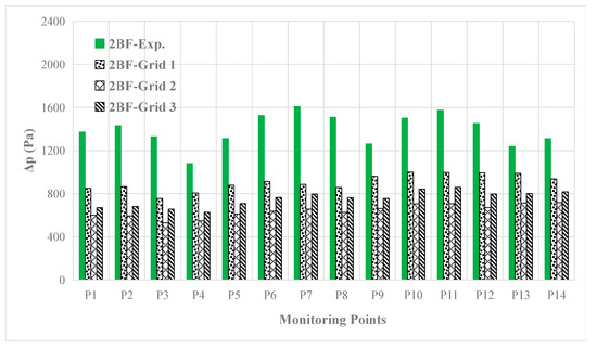
Figure 13. The 2BF component of hull pressure fluctuation predicted compared with the test data.

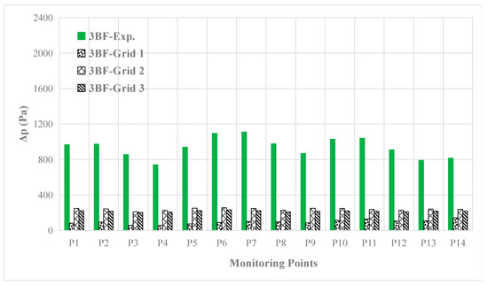
Figure 14. The 3BF component of hull pressure fluctuation predicted compared with the test data.

The influence of grid resolution on the hull pressure fluctuation at P10 is also assessed in Table 8. The predicted ΔP_S values using the three grids are all close to the experimental value, and the R_G obtained shows that the monotonic convergence was achieved for 0 < R_G < 1, the relative grid uncertainty U_G/S_C is also small, so all these predicted results illustrate the reliability of the numerical simulation methods again.

Table 8. The difference between prediction and measurement of 1BF component of hull pressure fluctuation ΔP_S, grid uncertainty U_G, and convergence ratio R_G.

Parameters	Grid 1	Grid 2	Grid 3	Experiment
ΔPS (Pa)	1672.0	1719.34	1962.8	1767.2
SC (Pa)	1624.6			-
Difference	−5.39%	−2.71%	11.07%	-
UG	35.9			-
UG/SC	2.210%			-
RG	0.194			-

5. Conclusions

The numerical simulation of propeller cavitation benchmark tests of the YUPENG ship model was conducted using the unsteady RANS approach based on OpenFOAM. The influence of grid resolutions on the unsteady propeller cavitation and hull pressure fluctuation was investigated in detail, and the conclusions obtained are as follows.

(1)

The thrust coefficients predicted using the three grids are all close to the measured value, the monotonic convergence was achieved, and the grid uncertainty is also quite small.

(2)

The difference of the cavity predicted among the three grids is not obvious, and Grid 2 can obtain satisfactory efficiency and precision of the unsteady propeller cavitation.

(3)

The 1BF components of the hull pressure fluctuation predicted using the three grids are all still close to the benchmark test value, the monotonic convergence was also achieved, and the grid uncertainty is quite small as well.

There are some aspects that remain to be studied further, such as the more accurate prediction of tip vortex cavity and cavity shedding at high frequency, which is the point that our subsequent study will focus on.

References

- Salvatore, F.; Streckwall, H.; Van Terwisga, T. Propeller Cavitation Modelling by CFD—Results from the VIRTUE 2008 Rome Workshop. In Proceedings of the First International Symposium on Marine Propulsors, Trondheim, Norway, 22–24 June 2009. [Google Scholar]
- Li, D.; Grekula, M.; Lindell, P.; Hallander, J. Prediction of Cavitation for the INSEAN Propeller E779A Operating in Uniform Flow and Non-Uniform Wakes. In Proceedings of the 8th International Symposium on Cavitation, Singapore, 13–16 August 2012; pp. 368–373. [Google Scholar]
- Paik, K.J.; Park, H.; Seo, J. URANS Simulations of Cavitation and Hull Pressure Fluctuation for Marine Propeller with Hull Interaction. In Proceedings of the 3nd International Symposium on Marine Propulsors, Launceston, Australia, 5–8 May 2013; pp. 389–396. [Google Scholar]
- Vaz, G.; Hally, D.; Huuva, T.; Bulten, N.; Muller, P.; Becchi, P.; Korsström, A. Cavitating Flow Calculations for the E779A Propeller in Open Water and Behind Conditions: Code Comparison and Solution Validation. In Proceedings of the 4th International Symposium on Marine Propulsors, Austin, TX, USA, 31 May–4 June 2015; pp. 330–345. [Google Scholar]
- Fujiyama, K.; Nakashima, Y. Numerical Prediction of Acoustic Noise Level Induced by Cavitation on Ship Propeller at Behind-Hull Condition. In Proceedings of the 5th Symposium on Marine Propulsors, SMP’17, Espoo, Finland, 12–15 June 2017; pp. 739–744. [Google Scholar]
- Long, Y.; Long, X.; Ji, B.; Huang, H. Numerical simulations of cavitating turbulent flow around a marine propeller behind the hull with analyses of the vorticity distribution and particle tracks. Ocean Eng. 2019, 189, 106310. [Google Scholar] [CrossRef]
- Yilmaz, N.; Aktas, B.; Sezen, S.; Atlar, M.; Fitzsimmons, P.A.; Felli, M. Numerical Investigations of Propeller-Rudder-Hull Interaction in the Presence of Tip Vortex Cavitation. In Proceedings of the 6th Symposium on Marine Propulsors, SMP’19, Rome, Italy, 26–30 May 2019; pp. 407–413. [Google Scholar]
- Asnaghi, A.; Feymark, A.; Bensow, R.E. Computational Analysis of Cavitating Marine Propeller Performance using OpenFOAM. In Proceedings of the 4th International Symposium on Marine Propulsors, Austin, TX, USA, 31 May–4 June 2015; pp. 148–155. [Google Scholar]
- Bensow, R.E. Large Eddy Simulation of a Cavitating Propeller Operating in Behind Conditions with and without Pre-Swirl Stators. In Proceedings of the 4th International Symposium on Marine Propulsors, Austin, TX, USA, 31 May–4 June 2015; pp. 458–477. [Google Scholar]
- Chaosheng, Z. The unsteady numerical simulation of propeller cavitation behind a single-screw transport ship using OpenFOAM. In Proceedings of the 2nd Conference of Global Chinese Scholars on Hydrodynamics, Wuxi, China, 20–23 November 2016; pp. 117–123. [Google Scholar]
- Chaosheng, Z. The numerical prediction of the propeller cavitation and hull pressure fluctuation in the ship stern using OpenFOAM. In Proceedings of the 5th Symposium on Marine Propulsors, SMP’17, Espoo, Finland, 12–15 June 2017; pp. 745–749. [Google Scholar]
- Menter, F.R. Two-equation eddy-viscosity turbulence models for engineering applications. AIAA J. 1994, 32, 1598–1605. [Google Scholar] [CrossRef]
- Issa, R.I. Solution of the implicitly discretised fluid flow equations by operator-splitting. J. Comput. Phys. 1986, 62, 40–65. [Google Scholar] [CrossRef]
- ITTC. CFD General Uncertainty Analysis in CFD Verification and Validation Methodology and Procedures. In ITTC Procedure 2002 7.5-03-01-01, Revision 01. Available online: https://www.marin.nl/storage/uploads/25027/files/7.5-03-01-01_ITTC_Uncertainty_proc_for_CFD.pdf (accessed on 10 August 2019).
- Roache, P.J. Verification and Validation in Computational Science and Engineering; Hermosa: Albuquerque, NM, USA, 1998. [Google Scholar]
- JCGM. Evaluation of measurement data—Guide to the expression of uncertainty in measurement, JCGM 100:2008 GUM 1995 with minor corrections. In Joint Committee for Guides in Metrology; Bureau International des Poids Mesures (BIPM): Sevres, France, 2008. [Google Scholar]
© 2019 by the authors. Licensee MDPI, Basel, Switzerland. This article is an open access article distributed under the terms and conditions of the Creative Commons Attribution (CC BY) license (http://creativecommons.org/licenses/by/4.0/).