Article

Infragravity Wave Energy Partitioning in the Surf Zone in Response to Wind-Sea and Swell Forcing

1
CSIRO Oceans and Atmosphere, Crawley 6009, Australia
2
Faculty of Science, School of Earth Sciences, The University of Western Australia, Crawley 6009, Australia
3
Departamento de Física, Universidad Nacional, Heredia 3000, Costa Rica
4
Faculty of Engineering and Mathematical Sciences, Oceans Graduate School, The University of Western Australia, Crawley 6009, Australia
*
Author to whom correspondence should be addressed.
J. Mar. Sci. Eng. 2019, 7(11), 383; https://doi.org/10.3390/jmse7110383
Submission received: 18 September 2019 / Revised: 22 October 2019 / Accepted: 23 October 2019 / Published: 28 October 2019
(This article belongs to the Special Issue Advances in Nearshore Hydrodynamics Research)

Abstract

:
An alongshore array of pressure sensors and a cross-shore array of current velocity and pressure sensors were deployed on a barred beach in southwestern Australia to estimate the relative response of edge waves and leaky waves to variable incident wind wave conditions. The strong sea breeze cycle at the study site (wind speeds frequently > 10 m s−1) produced diurnal variations in the peak frequency of the incident waves, with wind sea conditions (periods 2 to 8 s) dominating during the peak of the sea breeze and swell (periods 8 to 20 s) dominating during times of low wind. We observed that edge wave modes and their frequency distribution varied with the frequency of the short-wave forcing (swell or wind-sea) and edge waves were more energetic than leaky waves for the duration of the 10-day experiment. While the total infragravity energy in the surf zone was higher during swell forcing, edge waves were more energetic during wind-sea periods. However, low-frequency (0.005–0.023 Hz) edge waves were found to be dominant in absence of wind-sea conditions, while higher-frequency (0.023–0.050 Hz) edge waves dominated when wind-sea conditions were present.

1. Introduction

Infragravity (IG) waves, with frequencies ranging from 0.005 to 0.050 Hz (periods 20 s to 3 min), often account for an important part of the wave energy spectrum in the surf zone, and their energy increases with greater incoming short-wave height [1]. In intermediate water depths, spatial gradients in radiation stresses due to wave groupiness generate IG waves, referred to as bound (long) waves [2]. Bound waves propagate at the group frequency and are 180° out of phase with the wave group envelope outside of the surf zone. When wave groups approach the beach, the bound waves are said to be released, either when the wave groups break [3] or when the bound waves satisfy the free wave dispersion relationship [4,5]. Another mechanism for the generation of free IG waves in the nearshore is due to time-varying breakpoint forcing [6,7]. These dynamics have been numerically modelled [8] and reproduced in laboratory experiments [9,10,11], as well as observed in the field on beaches [5,12] as well as on fringing reefs [13].
Free incoming IG waves may reflect at the shoreline and then either propagate offshore as leaky waves or become refractively trapped to the shoreline as edge waves. Edge waves can be progressive or standing in the alongshore direction and are generally standing in the cross-shore direction. However, in the case of strong dissipation, edge waves can be also cross-shore propagating [14]. For plane beaches, the edge-wave amplitude is sinusoidal alongshore and decays exponentially in the offshore direction, with the number of nodes in the cross-shore surface elevation profile increasing with the edge-wave mode number. On barred beaches, edge waves can be trapped and amplified at the location of the bar [15,16], with a maximum in amplitude over the bar crest followed by an exponential decay offshore of the bar.
Oltman-Shay and Guza [17] observed that alongshore currents change the edge-wave dispersion relationship and Howd et al. [18] proposed a modified edge-wave dispersion relationship taking into account an alongshore current. They showed that the effect of an alongshore current is equivalent to a change of the bathymetry profile. Oltman-Shay and Howd [19] compare the frequency and wavenumber distribution of observed edge waves with model predictions of edge-wave solutions to the linear shallow water equations on nonplanar beach profile, taking alongshore currents into account. They found that the deviation from a planar beach profile and the presence of an alongshore current modified the cross-shore variance profile of edge waves in terms of the nodal structure and shoreline elevation estimation.
Standing IG waves contribute to the transport of suspended sediment and net sediment fluxes resulting from their motions can be large [20]. Alongshore progressive (cross-shore standing) edge waves may contribute to the formation and maintenance of alongshore-uniform sandbars [21,22]. However, the role of edge waves in bar formation and maintenance has not been conclusively demonstrated and Masselink et al. [23] demonstrated, in a case study, that edge waves were not a prerequisite to the development of beach cusps. An alternative approach known as self-organization provides an explanation for rhythmic features in the absence of forced alongshore periodicity of the incoming wave forcing [24,25,26,27].
Observations by Contardo and Symonds [28] at Secret Harbour, a low-energy barred beach in the southwestern Australia which is also the focus of this study, revealed that the sandbar was alongshore-uniform in the presence of obliquely incident wind-sea and alongshore currents, associated with sea breeze cycles, and remained alongshore-variable with normally incident wave forcing. Their study highlighted the role of wave incidence angle in regulating the alongshore-uniformity of the sandbar and they hypothesised sandbar straightening could occur through a mechanism involving progressive edge waves, since obliquely incident wave forcing favours the generation of edge waves over leaky waves [29] and alongshore currents are favourable to progressive edge waves [18,19].
Bowen and Guza [29] proposed a conceptual model based on two incoming short waves that generated a third wave with a frequency equal to the difference of frequencies between the two incoming short waves. They showed that for edge waves to be excited, they must satisfy a resonance condition, which is dependent on the bathymetry profile and the frequencies and incidence angles of the incoming short waves. They predicted that the infragravity wave energy partitioning along the edge wave and leaky-wave dispersion lines would depend on the period and direction of incoming short waves. However, these results have not been verified in field observations, as sites presenting a broad range of both incoming wave periods and directions are uncommon. We aim to verify these results at Secret Harbour, where a bimodal wave makes the site a particularly suitable location to do so.
In this study, we investigate the infragravity wave distribution in frequency and alongshore wavenumber space using measurements from a lagged alongshore array of pressure sensors and a cross-shore array of current meters, at Secret Harbour. At this site, obliquely incident wind-sea and normally incident swell alternately dominate throughout the day in the summer due to a strong diurnal sea breeze. This specific wave climate allows us to assess the dependence of the infragravity wave properties on the incident wave conditions.

2. Background

In this section, we provide background information on the theoretical distribution of edge-wave energy in frequency and wavenumber space, which provides a framework for the subsequent data analysis and interpretation.
The analytical edge-wave solutions to the linear shallow water equation of motion for a velocity potential Φ(x,y,t) over a plane beach [30] are:
Φ ( x , y , t ) = a n g σ cos ( k y ω t ) φ n ( x ) ,
where
φ n ( x ) = e k x L n ( 2 k x ) ,
in which an is the amplitude of the mode n edge wave at the shoreline, ω is the radial frequency, k is the alongshore wavenumber, x and y are the coordinates perpendicular (cross-shore) and parallel (alongshore) to the shoreline respectively, t is time, g is the gravitational acceleration and Ln are the Laguerre polynomials.
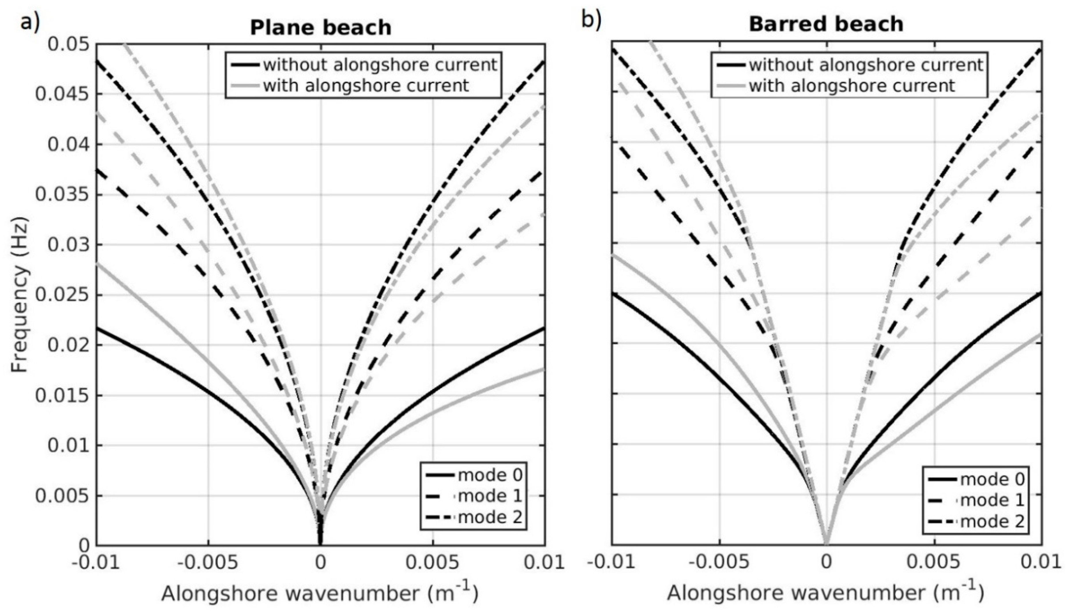
The derived edge-wave dispersion relationship for a plane beach (represented in black lines in Figure 1a) is:
ω 2 = g k ( 2 n + 1 ) β ,
where ß is the beach slope.
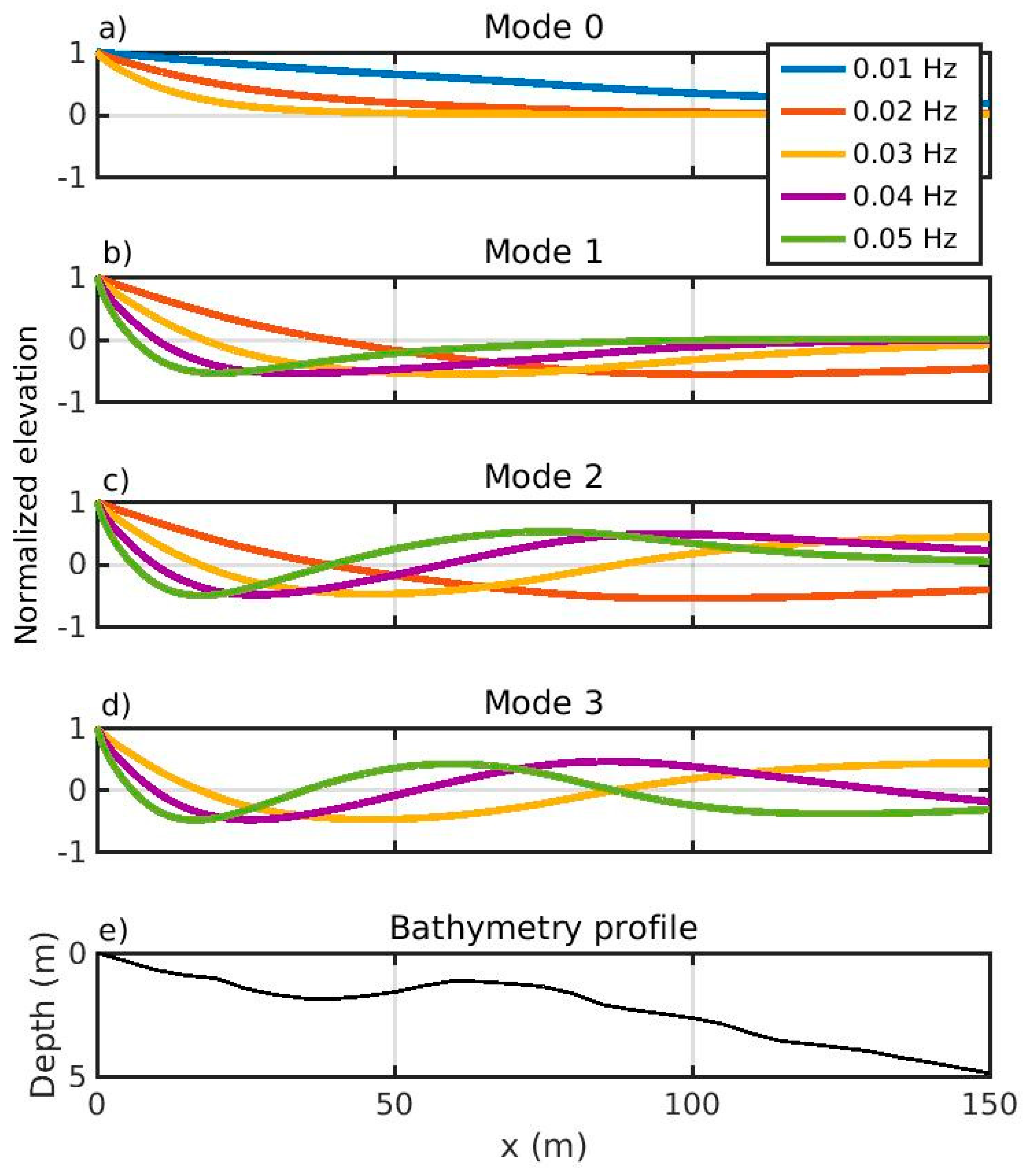
Following Holman and Bowen [31] and assuming a sinusoidal alongshore form of the progressive edge wave (Equation (1)), numerical solutions to the linear shallow water equations can be obtained for any arbitrary cross-shore bathymetry profile. The dispersion relationship curves calculated specifically for Secret Harbour, a barred beach, are shown in black lines in Figure 1b. The cross-shore profiles of the water elevation modes, with the amplitude normalized to unity at the shoreline, are represented on Figure 2 for waves of different frequency.
With the cross-shore (u) and alongshore (v) components of velocity, and elevation (η) defined by:
u = d Φ d x ;   v = d Φ d y ;   η = 1 g d Φ d t ,
this results in
u = a n g σ cos ( k y ω t ) d ϕ n ( x ) d x , v = a n g k σ sin ( k y ω t ) ϕ n ( x ) , η = a n sin ( k y ω t ) ϕ n ( x ) .
When an alongshore current is present, the edge-wave solutions are modified and the dispersion relationship is calculated following using an effective beach profile, h’(x), following [18]:
h ( x ) = h ( x ) [ 1 ( v ( x ) / c ) ] ,
where h(x) is the actual beach profile (different to β, which is the average beach slope), v(x) is the alongshore current profile and c is the edge-wave celerity. In the direction of (opposite direction to) the alongshore current, the bathymetry appears deeper (shallower) to the edge waves. The nodal structure shifts seaward (landward) and the dispersion curves are shifted toward lower (higher) absolute alongshore wavenumbers, as shown in Figure 1a for a plane beach and in Figure 1b for a barred beach. We estimated the cross-shore profile of the alongshore current from four measurements in a cross-shore array in the surf zone (see Section 3).

3. Methods

3.1. Field Experiment

A field experiment was conducted at Secret Harbour beach, a low-energy barred beach in the southwestern region of Western Australia (Figure 3), between 4 and 13 February 2014, when wave and wind conditions were typical of the austral summer period in the region. The site has a dominantly diurnal micro-tidal regime with a mean spring tidal range of 0.9 m. Four Nortek (Boston, MA, USA) Vector Acoustic Doppler Velocimeters (ADVs) were deployed in a cross-shore array at 40 m, 46 m, 60 m and 78 m (sites VEC1-4) from the shoreline in depths between 1 and 2 m (Figure 3d). The vectors sampled 7080 points at 2 Hz (59 min) each hour. A lagged alongshore array of RBR (Ottawa, ON, Canada) Virtuoso pressure sensors (sites P1–10) was deployed in the bar trough, about 30 m from the shoreline in about 2 m of water (Figure 3e,f) sampling continuously at 1 Hz. These pressure sensors were located at the following alongshore positions: y = −150, −138, −117, −77, −27, −13, −1, 15, 31, and 251 (Figure 3e,f). The lagged alongshore array was designed to cover a range of alongshore wavenumbers associated with edge waves (up to 0.01 m−1). One of the pressure sensors of the alongshore array (P3) was in line with the cross-shore array. A Nortek AWAC (Acoustic Wave and Currents) was also deployed 550 m offshore in 8 m of water and measured sea-surface elevation using Acoustic Surface Tracking (AST), collecting 8192 acoustic surface elevation measurements in 34-minute burst at 4 Hz every hour. The nearshore bathymetry was surveyed on 3 February (Figure 3e) and 14 February (Figure 3f) using a jet ski equipped with a single-beam echo sounder and RTK-GPS. The region surveyed was approximately −700 m < y < 700 m alongshore and 0 m < x < 350 m in the cross-shore. Wind speed and direction were measured at one-minute intervals with an anemometer mounted on top of the coastal station tower at a height of ~20 m above mean sea level (Figure 3c).

3.2. Wave and Wind Conditions

During summer periods, including during this field experiment, the wave climate in this region is characterized by consistent swell, of variable height, from the Southern Ocean as well as diurnal variations in wind-sea conditions associated with southwestern Australia’s strong sea breeze cycles [28]. For example, from 5 to 10 February, there were five consecutive sea breeze cycles, with wind speeds exceeding 15 m s−1 on both 7 and 10 February (Figure 4a), resulting in corresponding diurnal peaks in the significant wave height (Hm0) up to 1 m (Figure 4d) and spectral energy in the wind-sea band (0.125 to 0.5 Hz, Figure 4c). Two periods of larger swell (0.05 to 0.125 Hz, Figure 4c) occurred during the experiment (6–7 February and 12 February) with peak periods Tp above 8 s (Figure 4e) and a peak Hm0 of 0.5 m (Figure 4d). During sea breeze events, the wind direction was about 225° (oblique to the beach by 15°, see Figure 4b) and the wind-sea wave direction at the AWAC shifted towards the south compared with a mean swell direction of about 245°, (almost shore normal, see Figure 4f). The directional spreading (σθ) was smaller when swell was dominant (15° on average) compared to when wind-sea was dominant (19° on average). The obliquely incoming wind-sea generated strong northward alongshore currents exceeding 1 m s−1 on 7 February at VEC1 and VEC2 (Figure 4i). During the experiment the tidal range was 0.5 m (Figure 4f).

3.3. Wavenumber-Frequency Analysis

We used the Iterative Maximum Likelihood Estimate (IMLE) method, as described by Pawka [33] and Tsanis and Brissette [34], to calculate the alongshore wavenumber-frequency (f-ky) spectra from the pressure time series recorded by the lagged alongshore array (Figure 3b). A first approximation of the f-ky spectrum (S0) is given by the Maximum Likelihood Estimate (MLE) method using [35]:
S 0 ( k , ω ) = { n N m N Q n m 1 e i k ζ } 1 ,
where N = 10 is the total number of pressure sensors, Qnm is the matrix of pressure co-spectra between pairs of sensors m and n, ζ represents the corresponding lag distance and i is the imaginary unit.
However, the co-spectra reconstructed from S0 is not equal to the observed co-spectra. The Iterative Maximum Likelihood Estimate (IMLE) provides a better estimation of the observed co-spectra. The iteration starts with the reconstruction of the matrix of the co-spectra from Sj-1:
Q r e c , j = k = 0.01 0.01 S j 1 ( k , ω ) e i κ ζ d k .
A new estimated 2D-spectrum, Tj, is calculated using the MLE method, from the reconstructed co-spectra (Qrec,j). We obtain a further estimation of the spectra as:
S j ( k , ω ) = T j ( k , ω ) + ε j ,
with εj estimated as proposed by Oltman-Shay and Guza [17]:
ε j = | λ | α + 1 γ λ , λ = S 0 ( k , ω ) T j 1 ,
where α and γ are constants and α = 1 and γ = 20. The process is repeated until the normalised squared error (NSE) of the estimated co-spectra [33] satisfies:
N S E = ω k ( S N S N 1 ) 2 ω k S N 1 2 < 5 × 10 5 .
The f-ky spectra of pressure were calculated over three-hour periods. Three-hour periods were chosen to maximize the robustness of the f-ky spectra but over this time period the tidal variation remains small (less than 10 cm). We compare the f-ky spectra calculated from observations with the theoretical energy distribution in frequency and wavenumber described in Section 1.

4. Results

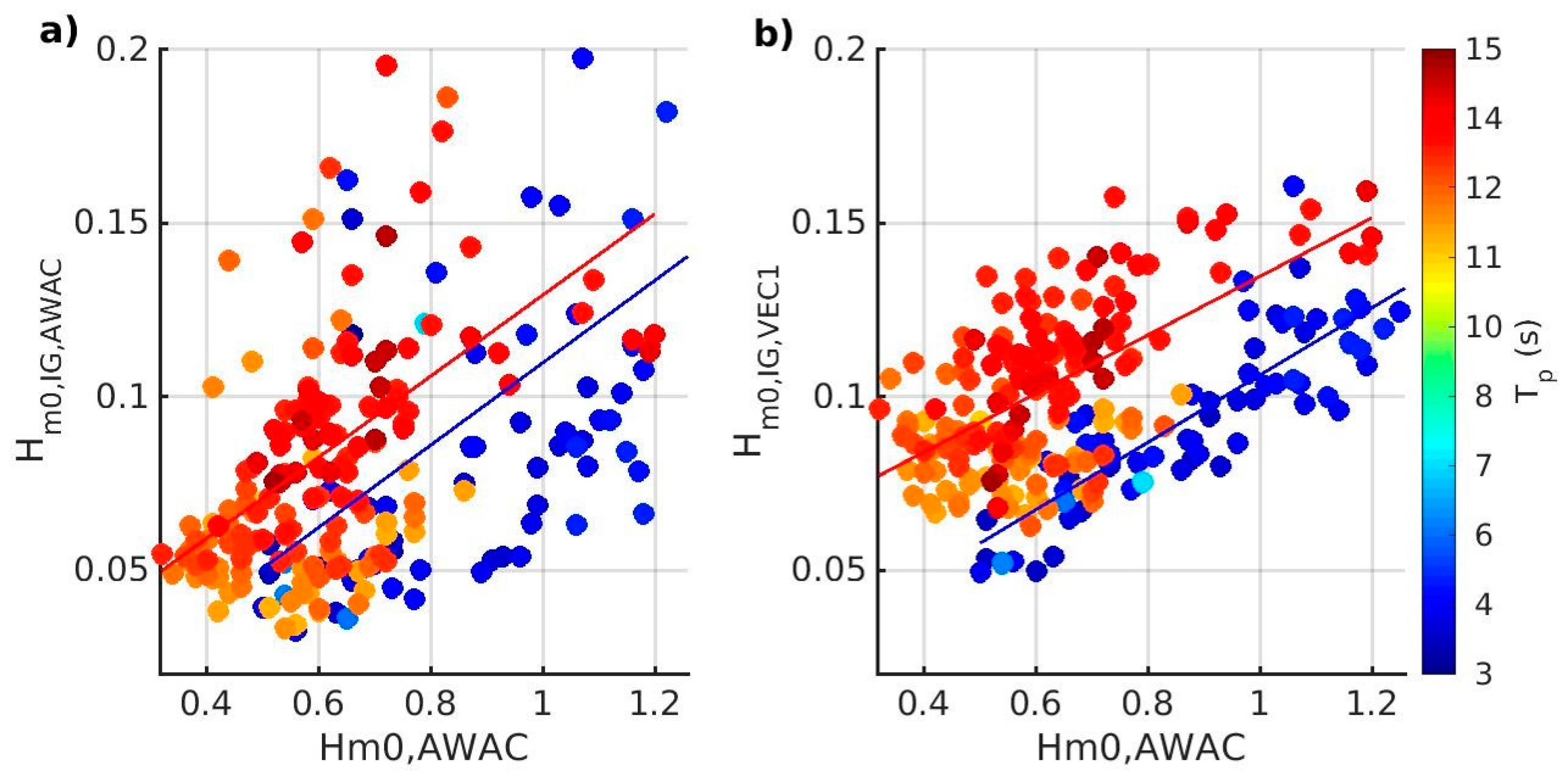
Figure 5 shows the observed IG wave height, at locations offshore (at the AWAC) and in the surf zone (at VEC1), versus swell and wind-sea wave height offshore, which reveals that when swell was dominant (Figure 5b, orange to red dots) the IG waves in the surf zone were larger that when wind-sea was dominant (Figure 5b, dark blue to cyan dots). Offshore at the AWAC, the amplitudes of the IG waves were only weakly dependent on the peak period of the offshore wave forcing (Figure 5a). However, in the surf zone, IG waves were larger when longer period swell was dominant than in wind-sea dominated conditions. This is consistent with prior observations made in the same location in 2009 [5].
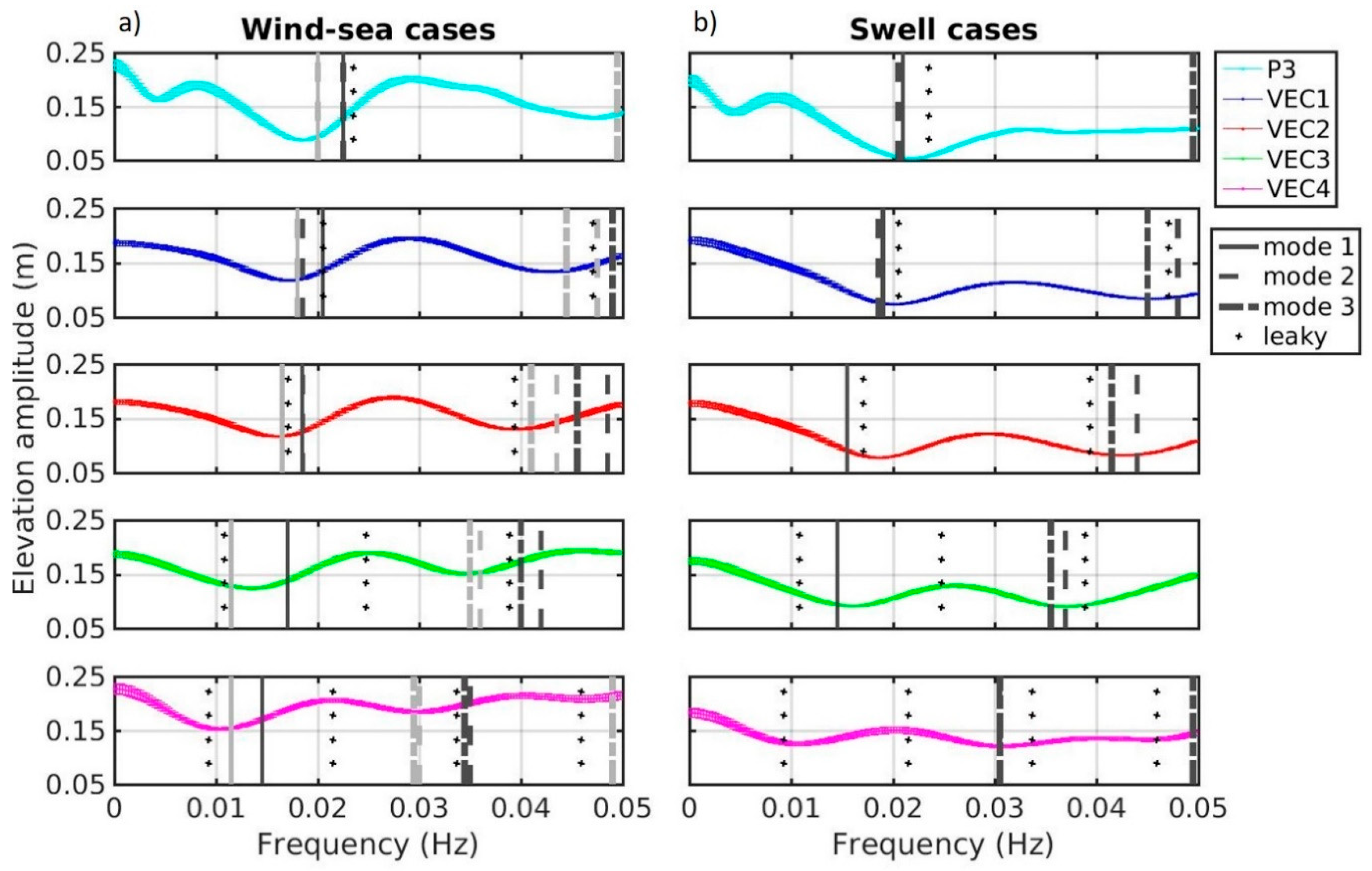
The frequency distribution of IG energy and the nodal structure vary with cross-shore location. Figure 6 shows the measured elevation amplitude at five cross-shore locations, calculated over three hours, for two cases: one when wind-sea was dominant and the sea breeze was strong; and one when swell was dominant. The measured elevation amplitudes include all IG waves (edge and leaky waves). The vertical lines represent the theoretical frequency of nodes in elevation for the first three edge-wave modes (Equation (5)) and cross-shore standing leaky waves. In the observations, the nodes appear as minima in elevation amplitude. The frequency of the theoretical edge-wave nodes corresponds to the minima in elevation amplitude in the measurements with a deviation of less than 0.005 Hz. The minima are not well defined since there is a combination of northward and southward-progressing edge-wave modes and leaky waves, and the bathymetry presents some alongshore variability which is not accounted for in the theoretical dispersion relationships. In the presence of an alongshore current, the nodes are shifted toward higher frequencies for edge waves propagating with the alongshore current [19]. This does not appear in the measurements from the cross-shore array since the nodes on 10 February (when alongshore currents were strong) are at lower frequencies than on 12 February. Close to the shore (P3), the nodal structure is better defined than away from the shore (VEC4). This representation provides information on the frequency distribution of IG energy at different cross-shore locations, but it does not provide information on the wavenumber distribution and does not distinguish between edge waves and leaky waves in the measurements.
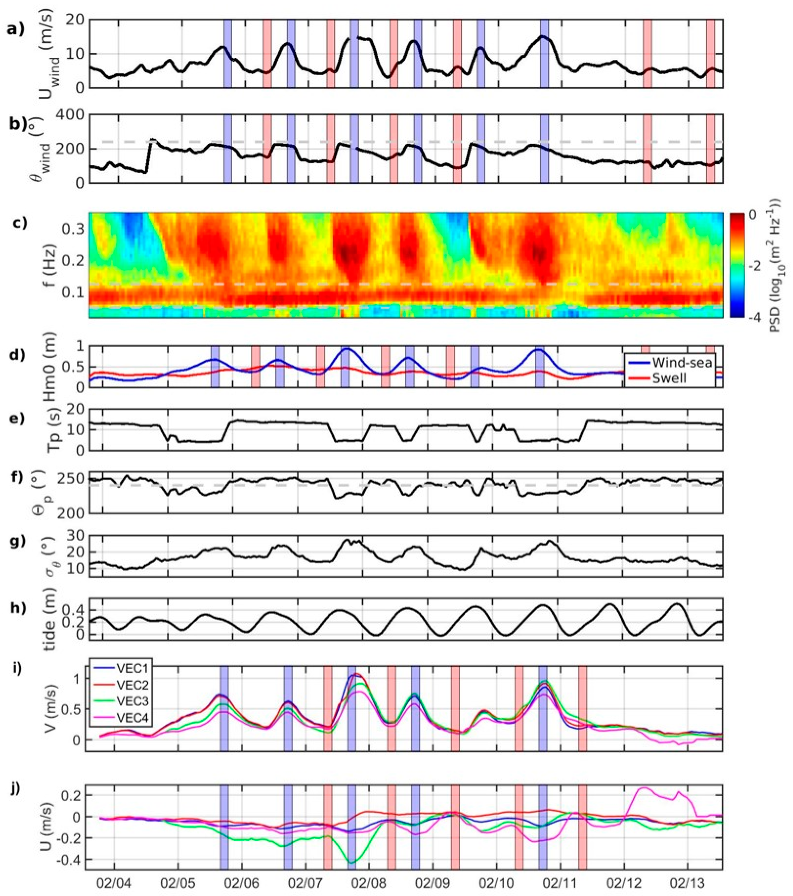
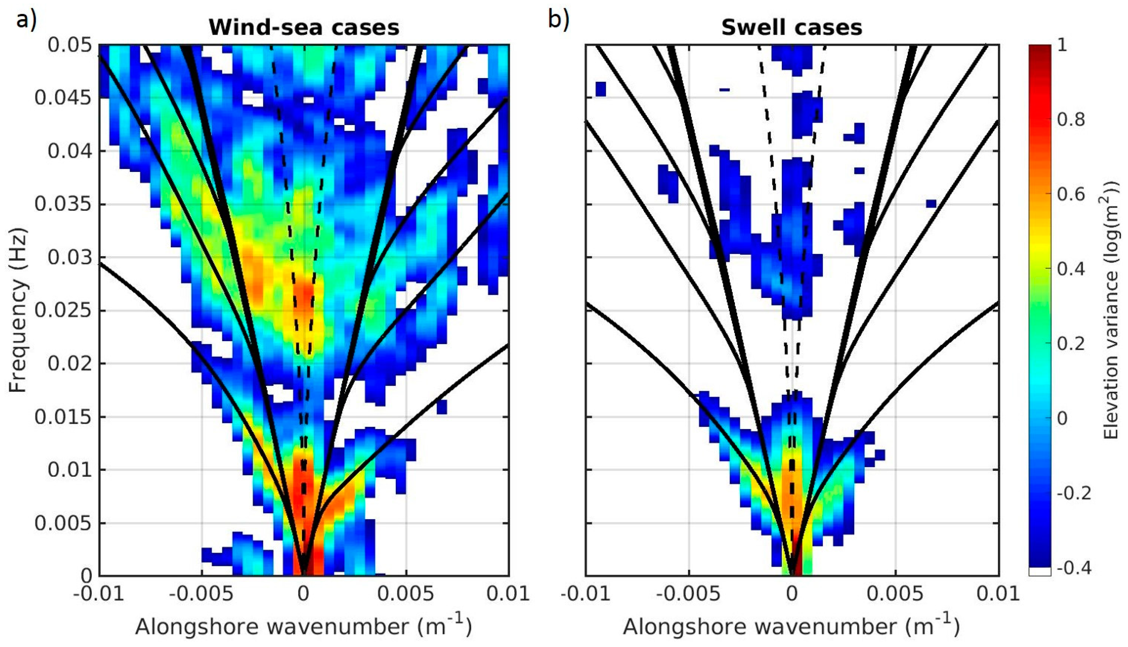
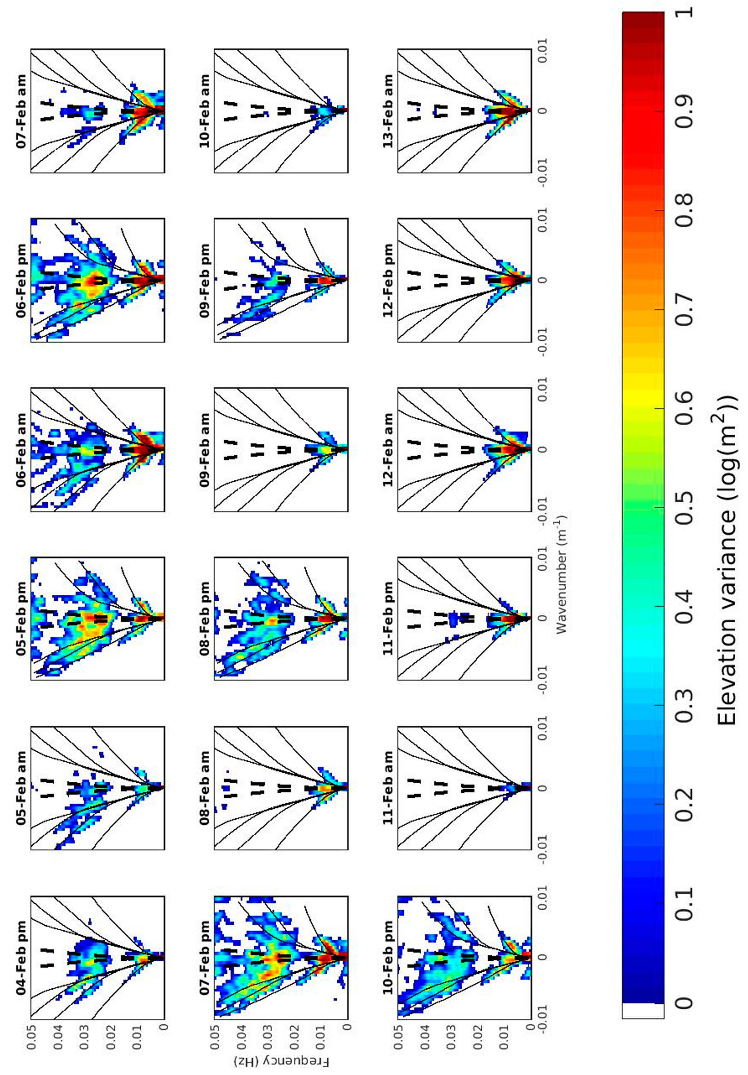
Using the pressure sensor measurements from the alongshore array, we compute f-ky spectra, and identify edge waves and leaky waves in the entire IG spectrum. Three-hour-averaged f-ky spectra are presented for wind-sea dominated conditions (5 to 10 February from 4 pm to 7 pm) and swell dominated conditions (6 to 9 and 12 to 13 February from 7 am to 10 am) and non-averaged f-ky spectra over 12-hour periods, from 1pm to 1am and 1am to 1pm (corresponding to sea breeze and swell dominated periods, respectively) are presented in Appendix A. The black solid lines in Figure 7 and Figure A1 represent the calculated edge-wave dispersion curves, with the measured alongshore current (~1 m s−1, Figure 4i) in the wind-sea cases (Figure 7a) and without alongshore current (observed to be < 0.1 m s−1, Figure 4i) in the swell cases (Figure 7b). Energy lying along the dispersion curves is indicative of edge waves while energy between the dashed lines indicates leaky waves. In the averaged wind-sea case (Figure 7a), there is an energy minimum at approximately 0.015 Hz suggesting the presence of an elevation node at the cross-shore location of the alongshore array of pressure sensors, consistent with cross-shore standing waves. At high IG frequencies, for both edge waves and leaky waves, higher peaks of energy are found during wind-sea forcing than during swell forcing (Figure 7).
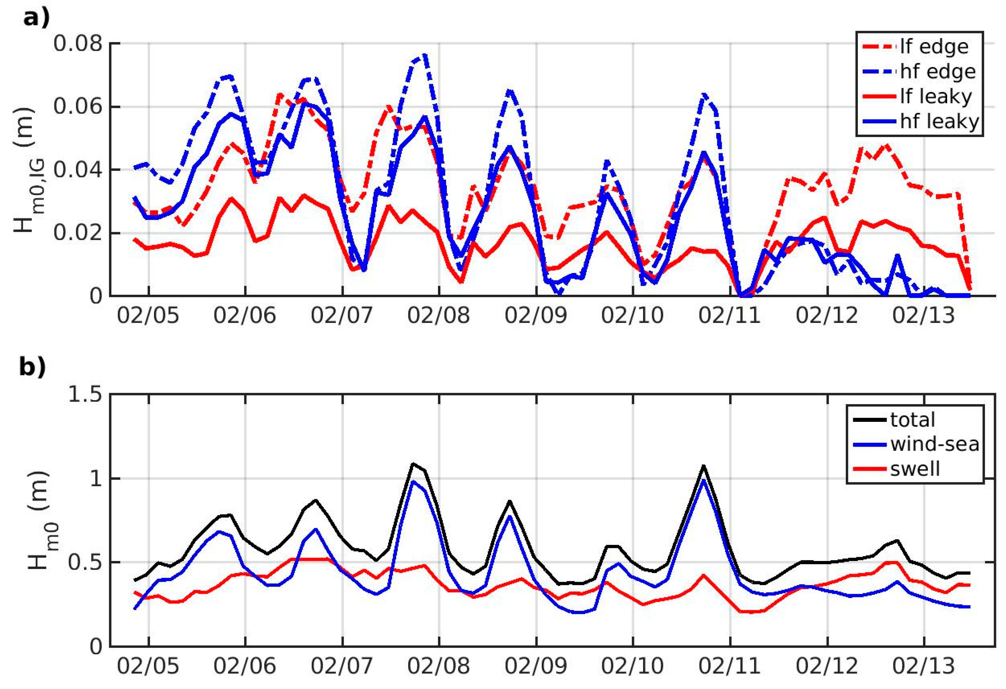
The IG significant wave height (Hm0,IG) extracted from non-averaged three hours f-ky spectra, indicates that edge waves generally dominated the energy spectrum over leaky waves throughout the experiment (Figure 8a). Figure 8b shows time series of significant wave height, for wind-sea (Hm0,sea), swell (Hm0,swell) and total (Hm0), averaged over the same three hour intervals to allow comparison with Figure 8a. From 5 to 10 February, strong sea breezes occurred in the afternoon each day and were associated with peaks of energy for high-frequency (high mode) edge waves. During the mornings of 6, 7 and 9 February, and on 12 and 13 February, wind-sea was relatively low and swell was dominant. Within this analysis, IG waves are separated into low-frequency (0.005 to 0.023 Hz) and high-frequency IG waves (0.023 to 0.050 Hz). The cut-off is chosen at 0.023 Hz because a node is present near this frequency at the cross-shore location of the alongshore array (Figure 6 and 
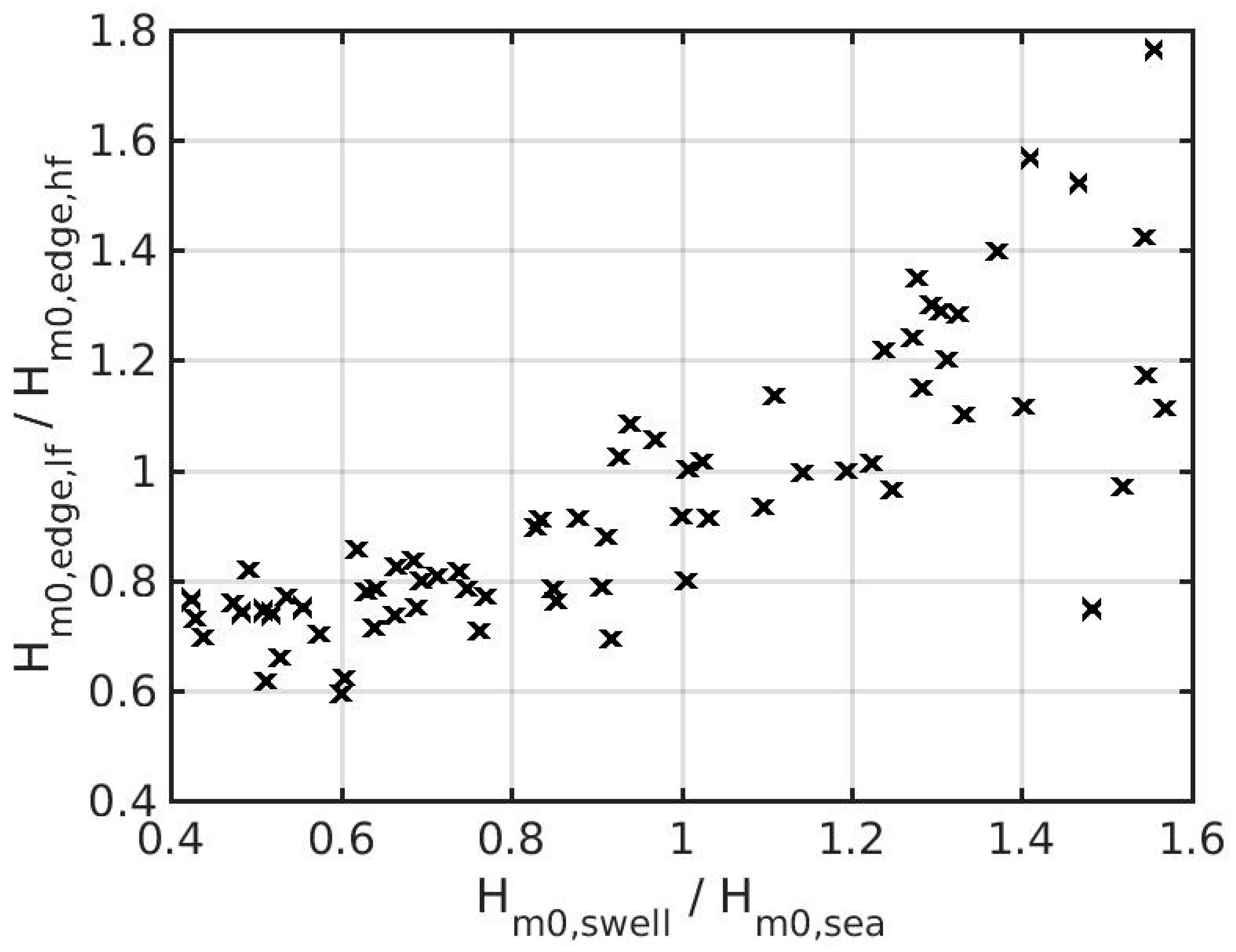
Figure 7). When swell was dominant, low-frequency edge waves dominated over high-frequency edge waves. This is represented with a scatter plot (Figure 9), where the ratio of low on high-frequency edge-wave heights is highly correlated (R = 0.82) with the ratio of the swell to wind-sea significant wave heights. This reveals that low-frequency edge waves dominated over high-frequency edge waves when swell conditions dominated over sea conditions. Table 1 summarises the correlation coefficients between the different components of Hm0,IG and Hm0 presented in Figure 8. Hm0,IG was highly correlated with Hm0 (Table 1 and Figure 5) and with the cross-shore current velocity U (Table 1). High-frequency IG energy (both edge and leaky) was well correlated with Hm0, Hm0,sea, U and V; whereas, low-frequency IG wave energy was highly correlated with Hm0,swell (Table 1). The IG waves were not as highly correlated with the tidal elevation as with the short-wave heights and currents (Table 1).
At Secret Harbour, the effects of the bar do not seem pronounced as we did not observe bar-trapped edge waves during this experiment. The elevation amplitude calculated following Holman and Bowen [31], for the Secret Harbour bathymetry profile, shows that no amplification of edge waves is expected over the bar (Figure 2). The measurements from the cross-shore array show no amplification over the bar either, as the elevation amplitude over the bar are of the same order of magnitude as the elevation amplitude close to the shoreline (VEC3 and P3 in Figure 6).

5. Discussion

We observed that low- and high-frequency IG waves responded differently to the short-wave forcing conditions driven by variability in the incoming swell and sea-breeze cycle. Low-frequency IG waves were well correlated with swell, while high-frequency IG waves were better correlated with the total short-wave height (Table 1). High-frequency edge waves dominated over low-frequency edge waves when wind-sea dominated over swell, and conversely (Figure 9). These results are consistent with the resonance conditions for edge waves proposed by Bowen and Guza [29].
Contardo and Symonds [5] previously observed at the same study site that IG waves appeared to be consistently generated by breakpoint forcing [7] independently of the short-wave forcing, and that during swell periods, the release of bound waves also occurred. Breakpoint forcing and bound wave release lead to different IG wave frequency distribution. This work could be extended to investigate whether the different IG wave generation mechanisms could have affected the IG wave partitioning observed in the present study.
The difference in IG wave partitioning may have consequences on beach morphology, and in particular on the alongshore variability. Previous work has shown that alongshore variability of the sand bar at Secret Harbour varied depending on the short-wave regime [28]. The sandbar was alongshore-uniform with wind-sea forcing and alongshore-variable with swell forcing. In the present study, we found that during wind-sea periods, high-frequency edge waves dominated over low-frequency edge waves (Figure 9). While IG waves may affect the beach morphology, there is no evidence so far that the edge waves may be responsible for the sand bar alongshore variability [23,25,26,27,36].
We found that the conditions for bar-trapping and amplification of edge waves are not met at Secret Harbour. Edge-wave modes with phase speeds approaching g h b a r , with hbar the depth over the bar, can potentially be trapped. However, the bathymetry at Secret Harbour, despite having a sandbar, was not conducive to the amplification of bar-trapped edge waves. In previous observations of bar-trapped edge waves at Duck, North Carolina [37] and Egmond aan Zee, Netherlands [38], the bars were in deeper water (2–4 m), so the phase speed of edge waves was higher on the bar than at Secret Harbour. In those locations, the edge waves satisfying the phase speed condition were of higher modes and presented antinodes which could be trapped and amplified by the bar. In the absence of bar-trapped edge waves maintaining the sandbar at Secret Harbour, alongshore variability may develop as soon as the alongshore current weakens [28].
Edge waves propagating northward (with the alongshore current) were up to 1.5 times the height of edge waves propagating southward However, the ratio of northward-propagating to southward-propagating edge-wave height was not correlated to the alongshore current velocity, nor the sea-swell wave height. According to the theoretical resonance conditions on wavenumber for edge waves [29], individual edge waves should propagate in the same alongshore direction as each pair of incoming short waves, therefore the ratio may be related to the directional spectral characteristics: incoming wave direction and directional spreading, i.e., a higher ratio would be expected during strong sea breeze conditions. However, we did not find any correlation between incoming wave directional characteristics and the ratio of edge waves propagating northward to edge waves propagating southward. The resonance conditions for edge waves do not explain the ratio of edge waves propagating in one direction to edge waves propagating in the opposite direction observed at Secret Harbour. This indicates that the role of the alongshore current is important, given that it produces the asymmetry in the frequency and wavenumber distribution of edge waves, which is necessary for edge waves to be alongshore progressive rather than standing.
Additional work, via detailed numerical modelling, is required to better understand the cause and effect relationships between the hydrodynamics associated with these observations and the morphological behaviour of the beach.

6. Conclusions

We observed the frequency-alongshore wavenumber distribution of edge waves and leaky waves on a barred beach with wave conditions alternating between periods with obliquely incident wind-sea, associated with sea breezes, and periods when normally incident swell dominated, in the absence of sea breeze. Our observations showed that edge waves were more energetic than leaky waves, and that low-frequency IG waves (0.005–0.0125 Hz) responded most strongly to the incident swell conditions; whereas, the high-frequency IG waves (0.0125–0.05 Hz) were well correlated with the total incoming short-wave height. The frequency and wavenumber distribution of IG waves depended on spectral and directional characteristics of the incoming short waves, as predicted from the resonance conditions for edge waves proposed by Bowen and Guza [29].

Author Contributions

Conceptualization, S.C., G.S., L.S., R.J.L. and J.H.; Methodology, S.C.; Software, S.C. and L.S.; Formal Analysis, S.C.; Investigation, S.C., G.S. and L.S.; Resources, R.J.L. and J.H.; Writing-Original Draft Preparation, S.C. and G.S.; Writing-Review & Editing, S.C., L.S., R.J.L. and J.H.; Funding Acquisition, G.S., R.J.L. and J.H..

Funding

Financial support for this research is provided by CSIRO, the University of Western Australia, the Royal Australian Navy as part of the Bluelink project, as well as an Australian Research Council Linkage Project grant (170100161) to RJL and JEH.

Acknowledgments

Field assistance was provided by Nick Mortimer, Daniel Kelsey-Wilkinson, Gundula Winter, Andrew Pomeroy, Mike Cuttler and Mark Buckley. Without their assistance this work could not have been completed. Thanks to Dirk Rijnsdorp for sharing his code to compute edge-wave elevation amplitude and dispersion lines. Thanks to Giovanni Coco for his feedback that has helped to improve the manuscript. Thanks to the anonymous reviewers, whose feedback has contributed to improve this manuscript.

Conflicts of Interest

The authors declare no conflict of interest.

Appendix A. f-ky Spectra

Figure A1. Elevation f-ky spectra, 12-hour averages. The colour bar denotes the elevation variance (m2 Hz−1 m−1), plotted on a logarithmic scale with lower values of elevation variance appearing in white. Black solid lines are theoretical dispersion curves (calculated based on the observed alongshore current at the time) and black dashed lines represent the cut-off between edge waves and leaky waves. Positive (negative) wavenumbers represent edge wave progressing southward (northward).
Jmse 07 00383 g0a1

References

  1. Holman, R.A. Infragravity energy in the surf zone. J. Geophys. Res. 1981, 86, 6442. [Google Scholar] [CrossRef] [Green Version]
  2. Longuet-Higgins, M.S.; Stewart, R.W. Radiation stress and mass transport in gravity waves, with application to ‘surf beats’. J. Fluid Mech. 1962, 13, 481. [Google Scholar] [CrossRef]
  3. Masselink, G. Group bound long waves as a source of infragravity energy in the surf zone. Cont. Shelf Res. 1995, 15, 1525–1547. [Google Scholar] [CrossRef]
  4. Baldock, T.E. Dissipation of incident forced long waves in the surf zone-Implications for the concept of “bound” wave release at short wave breaking. Coast. Eng. 2012, 60, 276–285. [Google Scholar] [CrossRef]
  5. Contardo, S.; Symonds, G. Infragravity response to variable wave forcing in the nearshore. J. Geophys. Res. Ocean. 2013, 118, 7095–7106. [Google Scholar] [CrossRef]
  6. Symonds, G.; Huntley, D.A.; Bowen, A.J. Two-dimensional surf beat: Long wave generation by a time-varying breakpoint. J. Geophys. Res. 1982, 87, 492. [Google Scholar] [CrossRef] [Green Version]
  7. Symonds, G.; Bowen, A.J. Interactions of nearshore bars with incoming wave groups. J. Geophys. Res. 1984, 89, 1953. [Google Scholar] [CrossRef]
  8. List, J.H. A model for the generation of two-dimensional surf beat. J. Geophys. Res. 1992, 97, 5623. [Google Scholar] [CrossRef]
  9. Baldock, T.E.; Huntley, D.A.; Bird, P.A.D.; O’Hare, T.; Bullock, G.N. Breakpoint generated surf beat induced by bichromatic wave groups. Coast. Eng. 2000, 39, 213–242. [Google Scholar] [CrossRef]
  10. Baldock, T.E.; Huntley, D.A. Long-wave forcing by the breaking of random gravity waves on a beach. Proc. R. Soc. A Math. Phys. Eng. Sci. 2002, 458, 2177–2201. [Google Scholar] [CrossRef]
  11. Baldock, T.E.; O’Hare, T.J.; Huntley, D.A. Long wave forcing on a barred beach. J. Fluid Mech. 2004, 503, 321–343. [Google Scholar] [CrossRef]
  12. Moura, T.; Baldock, T.E. Remote sensing of the correlation between breakpoint oscillations and infragravity waves in the surf and swash zone. J. Geophys. Res. Ocean. 2017, 122, 3106–3122. [Google Scholar] [CrossRef]
  13. Pomeroy, A.; Lowe, R.; Symonds, G.; Van Dongeren, A.; Moore, C. The dynamics of infragravity wave transformation over a fringing reef. J. Geophys. Res. Ocean. 2012, 117, 1–17. [Google Scholar] [CrossRef]
  14. Henderson, S.M.; Bowen, A.J. Simulations of Dissipative, Shore-Oblique Infragravity Waves. J. Phys. Oceanogr. 2003, 33, 1722–1732. [Google Scholar] [CrossRef]
  15. Kirby, J.T.; Dalrymple, R.A.; Liu, P.L.F. Modification of edge waves by barred beach topography. Coast. Eng. 1981, 5, 35–49. [Google Scholar] [CrossRef]
  16. Bryan, K.R.; Bowen, A.J. Edge wave trapping and amplification on barred beaches. J. Geophys. Res. C Ocean. 1996, 101, 6543–6552. [Google Scholar] [CrossRef]
  17. Oltman-Shay, J.; Guza, R. A data-adaptive ocean wave directional-spectrum estimator for pitch and roll type measurements. J. Phys. Oceanogr. 1984, 14, 1800–1810. [Google Scholar] [CrossRef]
  18. Howd, P.A.; Bowen, A.J.; Holman, R.A. Edge Waves in the Presence of Strong Longshore Currents. J. Geophys. Res. 1992, 97, 11357–11371. [Google Scholar] [CrossRef] [Green Version]
  19. Oltman-Shay, J.; Howd, P.A. Edge Waves on Nonplanar Bathymetry and Alongshore Currents—A Model and Data Comparison. J. Geophys. Res. 1993, 98, 2495–2507. [Google Scholar] [CrossRef]
  20. Aagaard, T.; Greenwood, B. Infragravity wave contribution to surf zone sediment transport—The role of advection. Mar. Geol. 2008, 251, 1–14. [Google Scholar] [CrossRef]
  21. Bowen, A.J. Simple models of nearshore sedimentation: Beach profiles and long-shore bars. Coastline Can. 1980, 1–11. [Google Scholar]
  22. Holman, R.A.; Bowen, A.J. Bars, bumps, and holes: Models for the generation of complex beach topography. J. Geophys. Res. 1982, 87, 457. [Google Scholar] [CrossRef]
  23. Masselink, G.; Russell, P.; Coco, G.; Huntley, D. Test of edge wave forcing during formation of rhythmic beach morphology. J. Geophys. Res. C Ocean. 2004, 109, 1–10. [Google Scholar] [CrossRef]
  24. Falqués, A.; Montoto, A.; Iranzo, V. Bed-flow instability of the longshore current. Cont. Shelf Res. 1996, 16, 1927–1964. [Google Scholar] [CrossRef]
  25. Deigaard, R.; Drønen, N.; Fredsøe, J.; Jensen, J.H.; Jørgensen, M.P. A morphological stability analysis for a long straight barred coast. Coast. Eng. 1999, 36, 171–195. [Google Scholar] [CrossRef]
  26. Falqués, A.; Coco, G.; Huntley, D.A. A mechanism for the generation of wave-driven rythmic patterns in the surf zone. J. Geophys. Res. 2000, 105, 24087–24971. [Google Scholar] [CrossRef]
  27. Coco, G.; Murray, A.B. Patterns in the sand: From forcing templates to self-organization. Geomorphology 2007, 91, 271–290. [Google Scholar] [CrossRef]
  28. Contardo, S.; Symonds, G. Sandbar straightening under wind-sea and swell forcing. Mar. Geol. 2015, 368, 25–41. [Google Scholar] [CrossRef]
  29. Bowen, A.J.; Guza, R.T. Edge Waves and Surf Beat. J. Geophys. Res. 1978, 83, 1913–1920. [Google Scholar] [CrossRef]
  30. Eckart, C. Surface Waves on Water of Variable Depth, 1951; Scripps Inst. of Ocean. Wave Rep. no. 100; ; ref. 51–12. Available online: https://repository.tudelft.nl/islandora/object/uuid:ab1ada31-db80-4601-8911-b261f36c2198/(accessed on 28 October 2019).
  31. Holman, R.A.; Bowen, A.J. Edge waves on complex beach profiles. J. Geophys. Res. 1979, 84, 6339. [Google Scholar] [CrossRef]
  32. Mortimer, N.; Symonds, G. Bluelink III Workpackage P4.2 Littoral-zone Field Program; CAWCR Technical Report series; 65; Centre for Australian Weather and Climate Research: Melbourne, Australia, 2013. [Google Scholar]
  33. Pawka, S.S. Island shadows in wave directional spectra. J. Geophys. Res. 1983, 88, 2579–2591. [Google Scholar] [CrossRef]
  34. Tsanis, I.K.; Brissette, F.P. A wave directional spectra program for wave gage arrays. Environ. Softw. 1991, 6, 151–160. [Google Scholar] [CrossRef]
  35. Davis, R.E.; Regier, L.A. Methods for estimating directional wave spectra from multi-element arrays. J. Mar. Res. 1977, 35, 453–477. [Google Scholar]
  36. Dodd, N.; Falques, A. A note on spatial modes in longshore current shear instabilities. J. Geophys. Res. 1996, 101, 22715–22726. [Google Scholar] [CrossRef]
  37. Bryan, K.R.; Howd, P.A.; Bowen, A.J. Field observations of bar-trapped edge waves. J. Geophys. Res. 1998, 103, 1285. [Google Scholar] [CrossRef]
  38. Rijnsdorp, D.P.; Ruessink, G.; Zijlema, M. Infragravity-wave dynamics in a barred coastal region, a numerical study. J. Geophys. Res. Ocean. 2015, 120, 4068–4089. [Google Scholar] [CrossRef]
Figure 1. Edge wave dispersion curves for a) a plane beach, β = 0.03, b) Secret Harbour beach averaged cross-shore profile (barred beach), without alongshore current (black) and with alongshore current (as measured during sea breeze periods) (gray) for the three first modes. Positive (negative) wavenumbers represent edge wave progressing southward (northward).
Jmse 07 00383 g001
Figure 2. (a) to (d) Cross-shore profiles of elevation, with amplitude at the shoreline taken as unity, for the first four edge wave modes, for four edge wave frequencies, calculated based on the Secret Harbour bathymetry during the study period; e) averaged cross-shore bathymetry profile measured at Secret Harbour.
Jmse 07 00383 g002
Figure 3. (a) Location of field experiment at Secret Harbour beach in southwestern Australia; (b) location of the beach in regard to the reef; (c) location of the Nearshore Research Facility and the location where the offshore wave conditions were measured by the AWAC (Acoustic Wave and Currents); (d) cross-shore bathymetry profile at the location of the cross-shore array (depths relative to mean sea level); (e) bathymetry on 3 February; (f) bathymetry on 14 February, with instrument positions superimposed on bathymetry. x and y represent the cross-shore and alongshore directions respectively, and the origin is the location of the Nearshore Research Facility, an observatory tower equipped with instruments to monitor the surf zone [32].
Jmse 07 00383 g003
Figure 4. Time series of (a) wind speed and (b) wind direction (The horizontal gray dashed line indicates the direction normal to the beach. Direction is in nautical convention.) measured at the anemometer. Direction is in nautical convention. (c) Spectrogram of elevation measured at the AWAC Acoustic Surface Tracking (AST) (The horizontal gray dashed line indicates the limits between infragravity (IG), swell and sea waves), time series of d) wave height, (e) peak period, (f) peak direction (The horizontal gray dashed line indicates the direction normal to the beach. Direction is in nautical convention.), (g) directional spreading (smoothed over three hours), (h) hourly tidal level, (i) alongshore current velocity (positive northward), (j) cross-shore current velocity (positive seaward). Data are smoothed over three hours. The periods studied are represented with blue (wind-sea cases) and red (swell cases) areas.
Jmse 07 00383 g004
Figure 5. IG wave height, (a) at the AWAC (offshore), (b) at VEC1 (surf zone), versus sea-swell wave height at the AWAC, colour coded by the peak period. Correlation coefficients (R) are (a) 0.50 for swell (red) and 0.48 for wind-sea (blue), (b) 0.61 for swell and 0.89 for wind-sea.
Jmse 07 00383 g005
Figure 6. Elevation amplitude versus frequency, averaged over (a) wind-sea cases (between 4 pm and 7 pm), (b) swell cases (between 7 am and 10 am), at five locations along the cross-shore array. Coloured lines are the measurements. The width of the lines represents the error (standard deviation). Vertical lines represent the theoretical frequency of nodes in elevation for three edge wave modes: n = 0 (black solid lines), n = 1 (black dashed lines), n = 2 (black dash-dot lines) and standing leaky waves (gray solid lines). For case a), both nodes for both northward (dark gray) and southward (light gray) propagating edge waves are represented.
Jmse 07 00383 g006
Figure 7. Elevation spectra averaged over (a) wind-sea cases (between 4 pm and 7 pm), (b) swell cases (between 7 am and 10 am). The colour bar denotes the elevation variance (m2 Hz−1 m−1), plotted on a logarithmic scale with lower values of elevation variance appearing in white. Black solid lines are theoretical dispersion curves (calculated based on the observed alongshore current at the time) and black dashed lines represent the cut-off between edge waves and leaky waves. Positive (negative) wavenumbers represent edge wave progressing southward (northward).
Jmse 07 00383 g007
Figure 8. (a) Time series of (a) Hm0,IG from the f-ky spectra (Appendix A, Figure A1), for two frequency ranges: 0.005–0.023 Hz (low frequency (lf), red and 0.023–0.050 Hz (high frequency (hf), blue) and for edge waves (dashed lines) and leaky waves (solid lines). (b) Significant wave height time series averaged over three hours, total (black), wind-sea (blue) and swell (red).
Jmse 07 00383 g008
Figure 9. Ratio of low-frequency to high-frequency edge wave height versus ratio of swell to wind-sea wave height.
Jmse 07 00383 g009
Table 1. Correlation coefficients, R, between different components of IG wave height (total, low frequency (lf), high frequency (hf), edge waves only, leaky waves only, low-frequency edge waves, high-frequency edge waves, low-frequency leaky waves and high-frequency leaky waves) with wave height (total, wind-sea, swell and ratio swell to wind-sea), current velocity and tidal elevation, based on three hourly observations. Note the current velocities represent cross-shore average values. High correlation coefficients are highlighted: green background indicates values ≥ 0.80 and yellow background indicates values between 0.75 and 0.80. In addition, the highest (absolute) coefficients in each column are underlined.
Hm0,IGTotallfhfEdgeLeakylf Edge hf Edgelf Leakyhf Leaky
Hm00.810.630.820.820.770.650.840.490.78
Hm0,sea0.730.450.800.730.700.470.820.330.74
Hm0,swell0.650.820.500.660.610.830.470.720.53
V (VEC1)0.700.380.800.700.670.400.820.280.74
U (VEC1)−0.80−0.73−0.76−0.81−0.76−0.74−0.76−0.60−0.75
tide0.500.460.480.520.470.440.510.490.42

