Abstract
Precise depth alignment of well logs is essential for reliable subsurface characterization, enabling accurate correlation of geological features across multiple wells. This study presents the Deep Hierarchical Graph Correlator (DHGC), a two-stage deep learning framework for scalable and automated well-log depth alignment. DHGC aligns a target log to a reference log by comparing fixed-size windows extracted from both signals. In the first stage, a one-dimensional convolutional neural network (1D CNN) trained on 177,026 triplets using triplet-margin loss learns discriminative embeddings of gammaray (GR) log windows from eight Norwegian North Sea wells. In the second stage, a feedforward scoring network evaluates embedded window pairs to estimate local similarity. Dynamic programming then computes the optimal nonlinear warping path from the resulting cost matrix. The feature extractor achieved 99.6% triplet accuracy, and the scoring network achieved 98.93% classification accuracy with an ROC-AUC of 0.9971. Evaluation on 89 unseen GR log pairs demonstrated that DHGC improves the mean Pearson correlation coefficient from 0.35 to 0.91, with successful alignment in 88 cases (98.9%). DHGC achieved an 8.2× speedup over DTW (3.16 s versus 25.83 s per log pair). While DTW achieves a higher mean correlation (0.96 versus 0.91), DHGC avoids singularity artifacts and exhibits lower variability in distance metrics than CC, suggesting improved robustness and scalability for well-log synchronization.
1. Introduction
Well-log data form the foundation of subsurface characterization, providing valuable insights into geological formations and reservoir dynamics that support exploration, development, and production decisions [1]. Precise data alignment is essential for minimizing errors in advanced reservoir simulations, including gas hydrate risk prediction [2], hydraulic fracturing analysis [3], and geothermal resource exploitation [4], and, in the context of subsurface characterization, accurate depth alignment of well-log measurements is critical for reliable reserve estimation, stratigraphic correlation, and well-completion planning [5]. In practice, however, significant depth mismatches frequently arise due to cable stretch, temperature variations, tool motion, and inter-tool differences [6,7]. These effects introduce nonlinear depth distortions, commonly referred to as stretch and squeeze, which, if uncorrected, obscure true geological relationships and can lead to costly misinterpretations [1,8].
A wide range of automated and semi-automated methods has been developed to address the depth-alignment problem. Early solutions relied on classical signal-processing techniques, such as windowed cross-correlation (CC) combined with dynamic programming for shift optimization, to determine the optimal depth shifts [9]. However, CC-based methods implicitly assume uniform, linear shifts and consequently perform poorly in the presence of stretch-and-squeeze distortions. Dynamic Time Warping (DTW) enables more flexible, nonlinear alignment but incurs quadratic computational complexity, limiting scalability to long logs or large datasets, and can generate geologically unrealistic one-to-many mappings when unconstrained. Constrained variants, such as Constrained DTW (CDTW) and Correlation Optimized Warping (COW), partially mitigate these issues by limiting the warping paths to physically reasonable alignments, preventing unrealistic shifts between the sequences [10]. Other approaches attempt to mimic human interpretation by identifying and matching discrete geological events [11] or by employing multi-scale feature-matching strategies [12]. Despite these advances, classical methods still face challenges, particularly when dealing with noisy data, repetitive lithologies, or cycle skipping.
These limitations have motivated a shift toward machine learning (ML) and deep learning (DL)–based approaches. Supervised learning formulations frame depth alignment as either a classification problem [13,14] or a regression task [1,15,16]. Convolutional Neural Networks (CNN) have demonstrated strong performance in both settings, with recent studies exploring multimodal fusion to improve robustness across logging conditions [17]. Hybrid architectures combining recurrent neural networks (RNNs) with wavelet decomposition have also been proposed to model sequential dependencies [18]. Unsupervised methods cluster dimensionally reduced log data to align lithological boundaries without labeled training data [19,20]. More recently, deep reinforcement learning (DRL) approaches have formulated depth alignment as a sequential decision-making problem, demonstrating effectiveness for large nonlinear misalignments [21,22].
Despite their methodological diversity, these advanced approaches share several fundamental limitations. First, data and generalization constraints arise because supervised classification relies on small, manually labeled anchor-point sets, making performance highly sensitive to labeling quality [13] and limiting generalization across log types and acquisition conditions [14]. Second, inability to capture complex distortions persists, as window-based formulations and piecewise-linear assumptions prevent modeling of stick-slip behavior, acceleration effects, and cumulative tool-motion errors [1,13]. Third, computational and interpretability challenges affect RL-based methods, which reduce labeling requirements but introduce high computational overhead, long training times, and opaque decision-making [21,22]. Finally, lack of physical constraints remains a critical issue, as most approaches do not integrate geologically plausible rules, increasing the risk of unrealistic alignments [23]. These limitations highlight a clear need for hybrid methods combining deep feature learning with transparent, physically constrained optimization.
Among existing alignment techniques, DTW remains one of the most accurate methods for handling nonlinear depth distortions, typically achieving higher correlation scores than alternative approaches [24,25]. However, its practical applicability is hindered by two fundamental challenges. First, quadratic computational complexity limits scalability to long logs or multi-well projects. Second, unconstrained warping paths may lead to pathological singularities (one-to-many mappings), in which individual samples are mapped across extended depth intervals, thereby violating geological continuity. Addressing these limitations while preserving DTW’s nonlinear alignment capability would enable a method that combines high accuracy with operational viability. CNNs offer a promising pathway in this regard: their effectiveness for geological feature extraction is well established [26], and learned similarity measures can replace sample-level distance computations, which dominate DTW’s computational cost. By operating on CNN-derived window embeddings and imposing explicit slope constraints on alignment paths, it becomes possible to retain DTW’s core principles while achieving substantial speedups and substantially reducing singularity artifacts.
Building on these insights, this paper introduces the Deep Hierarchical Graph Correlation (DHGC) framework, a two-stage architecture that integrates deep feature learning with constrained graph-based optimization. In the first stage, a CNN learns discriminative embeddings from local log windows, constructing a learned cost matrix that replaces handcrafted distance metrics. In the second stage, a constrained graph-based pathfinding algorithm identifies the optimal alignment path through this matrix, enforcing geological continuity while preventing one-to-many mappings. By decoupling local feature learning from global path optimization, DHGC achieves interpretability and computational efficiency under complex nonlinear distortions.
The principal contributions of this work are as follows. First, we introduce a learned cost matrix that replaces handcrafted distance measures with CNN-derived similarity scores, improving robustness to noise and amplitude variations in well logs. Second, we propose a graph-based pathfinding algorithm that enforces slope and monotonicity constraints through window-level matching, thereby inherently preventing the singularity artifacts commonly produced by unconstrained DTW. Third, we present a two-stage architecture that decouples feature learning from path optimization, improving interpretability while achieving an computational speedup over DTW. The framework is validated on 89 unseen log pairs, achieving a 98.9% success rate and increasing the mean Pearson correlation from 0.35 to 0.91.
The DHGC model is trained using manually depth-aligned GR curves from eight Norwegian North Sea wells, augmented with synthetic depth shifts. Performance is evaluated against CC and DTW using Pearson correlation, Euclidean distance, and Earth Mover’s Distance (EMD), which measures the cumulative distribution mismatch between aligned log signals.
The remainder of this paper is organized as follows. Section 2 describes data preparation, model architecture, and training methodology. Section 3 presents experimental results and comparative analysis. Section 4 discusses implications and limitations, and Section 5 concludes with directions for future research.
2. Methodology
This section details the proposed DHGC framework, including data preprocessing, model architecture, training protocol, and the alignment algorithm.
2.1. Problem Formulation
Let the reference well log be and the target log , where and denote measured depths (m) and are the corresponding log measurements. Both depth sequences are strictly increasing.
The objective of depth alignment is to find an admissible warping path
minimizing the cumulative dissimilarity:
where is a learned local cost function.
To ensure geological plausibility and avoid the singularity artifacts common in standard DTW, the path P is subject to strict monotonicity and slope constraints. Unlike standard DTW, which permits orthogonal moves that lead to infinite stretching, DHGC enforces an 8-connectivity neighborhood constraint (detailed in Section 2.8). This bounds the local stretch/squeeze ratio, designed to respect the physical limits of geological deformation.
The optimal path defines a monotone depth mapping , yielding the aligned log:
2.2. Data Preprocessing
A standardized preprocessing pipeline is applied to all well log pairs [27]. Well-log data are loaded from LAS or CSV files, and rows with null values or duplicate depths are removed. Each log pair is trimmed to the common overlapping depth interval and interpolated onto a uniform grid of 0.1524 m. GR values are independently scaled to using min-max normalization:
2.3. Training Data and Generalizability
The training dataset consists of eight manually depth-aligned GR log pairs acquired from Electric Wireline (EWL) and Logging While Drilling (LWD) tools in wells from the Norwegian North Sea. GR logs were selected due to their ubiquity in the region and high vertical resolution, which provides well-defined stratigraphic tie-points for alignment.
The proposed DHGC framework is designed to be signal-type independent at the architectural level, as it operates on min–max normalized scalar inputs (Section 2.2). As a result, the method is mathematically compatible with other scalar well-log measurements. From a physical perspective, log types exhibiting variation patterns similar to GR may be directly amenable to the current pre-trained model; however, such transferability has not been evaluated in this study. For log types with fundamentally different morphological characteristics, such as the blocky responses typical of resistivity logs or the distinct noise characteristics of density measurements, retraining is required to enable the feature extractor to learn measurement-specific patterns.
Following preprocessing, the log sequences range from 450 to 18,498 samples, encompassing a wide variety of geological contexts. Each log is segmented into overlapping windows of 128 samples (∼19.5 m) with a stride of one sample. For a log of length N, this results in windows. The window length of 128 samples was selected based on an ablation study (Section 4.2).
2.3.1. Feature Extractor Training Data
For each depth-aligned log pair, the EWL window sequence serves as anchors, while the corresponding LWD sequence provides positive matches. A negative window is generated by sampling an LWD window at index , with the offset drawn uniformly from the range samples, corresponding to ±7.6 m at the 0.1524 m sampling interval.
Each training example therefore forms a triplet . Across the eight wells considered, this procedure yields 177,026 triplets, which are split into 60% training, 20% validation, and 20% testing sets.
The -sample offset range is motivated by both operational depth uncertainties and geological considerations. Reported wireline depth errors typically lie in the range of 1–10 m, with most misalignments below approximately 8 m [6,28]. Given the selected window length of 128 samples (∼19.5 m), offsets up to 7.6 m produce hard negatives that remain geologically similar to the anchor window while representing incorrect depth correspondence. Larger offsets increasingly correspond to distinct stratigraphic intervals, introducing repetitive or ambiguous lithological patterns that weaken the discriminative signal during training.
Preliminary experiments indicated that narrower offset ranges yield insufficient hard negatives, whereas wider ranges produce either trivially separable or geologically ambiguous negatives that degrade embedding quality. Importantly, large cumulative depth distortions are not modeled at the window level but are recovered through the subsequent global graph-based alignment stage, where sequences of locally consistent matches collectively correct substantial depth mismatches. Consequently, constraining local offsets is not expected to limit the method’s ability to recover realistic depth misalignments.
2.3.2. Scoring Model Training Data
After training, the feature extractor weights are frozen. For each index i, a positive pair is formed as with label , and a negative pair as with label , where is randomly selected. This produces 354,052 feature pairs, split 60/20/20 for training, validation, and testing.
2.4. Design Rationale
The DHGC architecture explicitly separates local feature invariance (Stage 1) from global nonlinear warping (Stage 2). These stages are linked through a compact embedding representation that transforms window-level similarities into a global alignment cost structure.
2.4.1. Stage 1: Local Feature Invariance
The CNN is trained using depth-shifted window pairs with offsets in the range samples, rather than synthetically stretched or compressed signals. At the selected window length of 128 samples (∼19.5 m), real-world depth distortions are approximately linear, with reported stretch and squeeze ratios rarely exceeding 5–10% [6]. Under these conditions, local deformations primarily manifest as amplitude and phase variations, which are effectively absorbed by convolutional filters and pooling operations. As a result, the CNN is designed to learn embeddings that are approximately invariant to small local depth shifts while preserving geological shape information.
2.4.2. Dimensionality Reduction
Each 128-sample window is mapped to a 32-dimensional embedding vector . This fourfold dimensionality reduction substantially lowers computational cost in the subsequent pairwise scoring and graph construction while suppressing high-frequency noise and redundant information. The reduced embedding preserves the essential morphological characteristics of the log response required for reliable matching. After alignment, window-level tie-points are projected back to the original depth grid via linear interpolation.
2.4.3. Stage 2: Global Nonlinear Alignment
Large-scale nonlinear depth distortions are resolved in Stage 2 using a constrained graph-based minimum-cost path algorithm (Section 2.8). Operating on the window-level similarity scores derived from the learned embeddings, the graph formulation accumulates many locally consistent matches to recover variable stretch and squeeze behavior, including cumulative distortions that exceed the length of individual windows. This global optimization is designed to enforce physical continuity and reduce the likelihood of implausible one-to-many correspondences. The complete dimensional flow through the DHGC pipeline is summarized in Table 1.

Table 1.
Dimensional flow through the DHGC pipeline.
2.5. External Test Set
The external test set comprises 89 previously unseen GR log pairs (EWL reference, LWD target) from the Norwegian North Sea, ranging from approximately 200 to over 10,000 samples. These are raw field data exhibiting noise, missing values, sampling irregularities, and nonlinear depth shifts. Preprocessing follows Section 2.2.
2.6. Model Architecture
The DHGC framework is composed of two core neural network components: a feature extractor and a scoring model.
2.6.1. Feature Extractor
The feature extractor is a 1D CNN mapping a 128-sample GR window to a 32-dimensional embedding. The architecture comprises three convolutional blocks with ReLU activations [29]: the first layer (16 filters, kernel size 5, padding 2) and second layer (32 filters, kernel size 3, padding 1) are followed by max-pooling [30], while the third layer uses 64 filters (kernel size 3, padding 1). The output is flattened and projected through two fully connected layers (128 and 32 units) to produce .
2.6.2. Scoring Model
The scoring model is a feedforward network accepting concatenated embeddings . It comprises two hidden layers (64 and 32 units) with ReLU activations and 20% dropout after the first layer. The output layer is a single sigmoid neuron producing match probability .
2.7. Model Training
The model is trained in a two-stage process designed to first learn robust data representations and then learn how to compare them. If a pre-trained model is not available, the script prepares the training data from the available depth-aligned logs, following the process described in Section 2.3.
2.7.1. Stage 1: Feature Extractor
The model is trained using the triplet dataset described in Section 2.3.1. The objective is to learn a discriminative embedding space in which geologically equivalent windows (Anchor and Positive) are mapped close together, while stratigraphically distinct windows (Negative) are mapped farther apart.
This objective is enforced using the triplet margin loss:
where is a fixed margin. The loss does not target absolute feature values, but instead penalizes violations of relative similarity: it is nonzero only when a geologically mismatched window is closer to the anchor than a matched window by at least the margin.
During optimization, minimizing this loss reduces the anchor–positive distance and increases the anchor–negative distance whenever the margin constraint is violated. This implicitly drives the CNN to become invariant to non-geological perturbations (e.g., tool-specific differences between EWL and LWD) while emphasizing morphological features that distinguish stratigraphic intervals, such as peak shapes and relative motif ordering. Once the margin condition is satisfied for a triplet, the loss becomes zero and no further updates are applied for that sample.
Training uses the Adam optimizer with a learning rate of , a batch size of 64, and 100 epochs with early stopping.
2.7.2. Stage 2: Scoring Model
With the feature extractor weights frozen, the scoring model is trained to classify pairs of embedding vectors as matching or non-matching using binary labels (1 for match, 0 for mismatch). Model parameters are optimized by minimizing the binary cross-entropy (BCE) loss:
where denotes the ground-truth label and is the predicted match probability. The scoring network is trained using the same optimization settings as the feature extractor. Figure 1 summarizes the overall workflow.
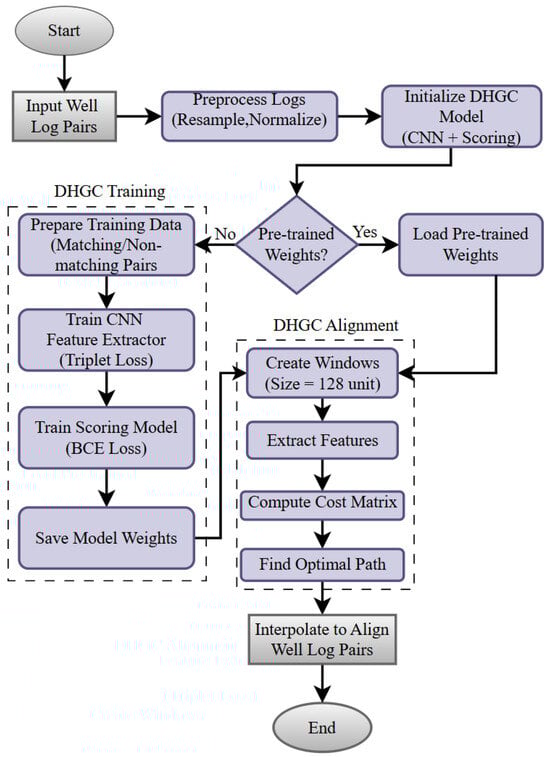
Figure 1.
DHGC workflow. Left: training phase. Right: alignment phase.
2.7.3. Overfitting Prevention
Overfitting is reduced using four strategies: (1) CNN weights are frozen to prevent co-adaptation between stages; (2) negative pairs for the scoring model are sampled randomly to expose the model to unseen combinations; (3) a 20% dropout is applied to reduce memorization; (4) training is stopped early if the validation loss does not improve for 10 consecutive epochs.
2.8. DHGC Alignment Algorithm
Once the DHGC model is trained, it is used to align new well log pairs. While this workflow shares the same underlying concept as standard DTW, it fundamentally replaces both the cost calculation and the pathfinding mechanism. Specifically, it substitutes the simple mathematical distance of standard DTW with a learned, intelligent assessment of similarity. Furthermore, it replaces the rigid dynamic programming search with a sophisticated graph-based algorithm. This global optimization approach is more robust and handles unequal log lengths more effectively than traditional methods. The procedure consists of four steps:
2.8.1. Step 1: Feature Extraction
First, the reference log and target log are sliced into overlapping windows of 128 samples. The pre-trained CNN feature extractor processes each window to create a compact fingerprint (feature vector ).
This results in a sequence of n feature vectors for the reference log, denoted as , and m vectors for the target log, .
The purpose of this step is to reduce noise and improve organization. Because the CNN was trained with triplet margin loss, it is trained to reduce sensitivity to random noise and compress the complex signal shape into a clean 32-dimensional vector. This structured organization of features can simplify the task for the subsequent scoring model, ensuring that it receives clean, meaningful representations rather than raw, noisy data.
2.8.2. Step 2: Cost Matrix Construction: Calculating Match Probabilities
Next, we build an cost matrix to map out where the logs match. Instead of calculating a simple distance (like Euclidean distance), we use the trained Scoring Model. For every possible pair consisting of the k-th reference window and the l-th target window, the Scoring Model inputs their feature vectors and predicts a probability of a match (). We convert this probability into a cost using the formula:
If the model is confident that the windows match (high probability), the cost is near zero. If they do not match, the cost is high. This creates a detailed map where valleys (low costs) represent the correct alignment path.
2.8.3. Step 3: Graph-Based Path Finding
The alignment problem is solved as shortest-path search through a weighted graph using Dijkstra’s algorithm via route_through_array [31,32].
Unlike standard DTW with 3-connectivity , DHGC employs 8-connectivity:
Combined with monotonicity (, ), this limits local slope to , corresponding to maximum 2:1 stretch/squeeze ratio, which is geologically plausible for well-log depth corrections [33].
2.8.4. Step 4: Depth Mapping and Interpolation
Window indices in path P are converted to physical depths using window-center coordinates, providing tie-points between reference and target depths. Linear interpolation between tie-points and nearest-neighbor extrapolation at edges produce the final aligned curve. This reconstruction naturally accommodates non-linear stretch and squeeze deformations through varying tie-point intervals, while the underlying graph constraints are designed to reduce the singularity artifacts (step-like discontinuities) characteristic of unconstrained DTW.
2.8.5. Singularity Avoidance
DHGC avoids DTW singularities through multiple mechanisms. First, the CNN embeddings produce smooth gradients, ensuring the cost matrix remains continuous and preventing sharp discontinuities that could trap DTW in degenerate paths. Second, operating on 128-sample windows enforces window-level granularity, which avoids one-to-many mappings at the individual sample level. Finally, an implicit slope constraint via 8-connectivity with monotonicity limits extended horizontal or vertical moves, such that
2.8.6. Tie-Point Density and Interpolation Validity
With stride 1, consecutive tie-points are separated by 0.1524 m—the same as the sampling interval. It is important to distinguish this tie-point density from the effective resolution, which is governed by the 128-sample window size (∼19.5 m receptive field). While a 128-sample window implies a receptive field of ∼19.5 m, the overlapping sliding-window approach ensures that depth shifts are updated incrementally at every sample step. Visual inspection of aligned results (e.g., Pair 10) confirmed that linear interpolation between these tie-points does not introduce significant stair-step artifacts or residuals in nominal cases. This is because the 1D CNN implicitly acts as a low-pass filter, focusing alignment on geologically significant structural trends rather than high-frequency noise. Consequently, linear interpolation accurately reconstructs the depth mapping for the majority of log intervals, with failures occurring only in rare cases of extreme high-frequency variability combined with short log segments (as analyzed in Section 3.3.2).
2.8.7. Data Length Constraints and Edge Effects
The fixed-input architecture of the 1D CNN requires input sequences of exactly 128 samples. While sequences shorter than this window could theoretically be handled via zero-padding, this introduces artificial signal values that distort feature embeddings and degrade the reliability of the cost matrix. Furthermore, in operational settings, log segments shorter than 128 samples (∼19.5 m) are typically artifacts of tool tests or fragmented runs and lack sufficient geological context for meaningful correlation. Therefore, any log segment shorter than the window size is strictly excluded from the analysis.
Additionally, inherent edge effects occur at the beginning and end of valid log sequences. Because tie-points are defined at the center of each sliding window, the first and last 64 samples (∼9.8 m) of any log lack direct tie-point coverage. For these regions, the alignment is handled via linear extrapolation based on the slope of the nearest valid window pair.
For robust performance, we recommend that log segments exceed 256 samples (∼39 m) with at least 50% depth overlap. Segments between 128 and 256 samples are processed; however, the limited number of resulting tie-points may reduce the stability of the graph-based pathfinding, leading to suboptimal predictions.
For log termini with fewer than 64 samples before the first (or after the last) window center, tie-points are extrapolated using the slope from the nearest valid pair, affecting approximately 9.8 m at each end.
2.9. Evaluation Metrics
2.9.1. Model Performance Evaluation
Before performing alignment, it is crucial to verify that the neural networks have learned robust representations and are not overfitting to the training data. We evaluate the two stages of the DHGC architecture using distinct classification metrics on a held-out test set.
Feature Extractor Evaluation (Triplet Accuracy): To assess the quality of the embedding space generated by the CNN, we measure Triplet Accuracy. For a given triplet (anchor, positive, negative), the model is considered correct if the Euclidean distance between the anchor and the positive sample is smaller than the distance between the anchor and the negative sample:
where is the indicator function. A high accuracy indicates that the model successfully clusters similar geological patterns while separating dissimilar ones [34].
Scoring Model Evaluation (ROC-AUC): The Scoring Model is a binary classifier predicting whether two windows match. We evaluate its performance using the Area Under the Receiver Operating Characteristic Curve (ROC-AUC) [35]. This metric is preferred over simple accuracy as it measures the model’s ability to rank true matches higher than mismatches across all classification thresholds, providing a robust measure of separability independent of class balance. An AUC score close to 1.0 indicates excellent discrimination capability.
2.9.2. Alignment Quality Evaluation
Once the models are validated, they are applied to the alignment task. The quality of the final alignment is evaluated by comparing the values of the reference log, , with the corresponding values of the aligned target log, , as defined in Section 2.1. For clarity in the formulas below, we denote these sequences as vectors:
Pearson Correlation Coefficient: Measures the linear similarity between the reference log and the aligned target log. It is defined as:
where and are the mean values of the respective logs. A value of 1 indicates a perfect positive linear relationship [36].
Euclidean Distance: Quantifies the cumulative pointwise difference between the two logs:
Lower values indicate a closer match between the aligned logs [37].
Earth Mover’s Distance (EMD): Measures the dissimilarity between the value distributions of the two logs. The logs are treated as histograms by first clipping values at zero and then normalizing to form probability distributions and :
EMD calculates the minimum work required to transform distribution into :
subject to the constraints , , and , where is the transport plan (or flow matrix) and is the ground distance. Lower EMD values indicate better distributional similarity [38].
Additionally, the computation time for each alignment method (DTW, CC, and DHGC) is recorded to evaluate its computational efficiency.
2.10. Baseline Methods
The proposed DHGC method is compared with two baseline depth alignment models, CC and DTW, to evaluate its performance on GR log pairs from EWL and LWD tools across 89 test pairs from the Norwegian North Sea.
2.10.1. Cross-Correlation Alignment
Cross-correlation (CC) identifies the optimal global linear shift by maximizing the similarity between the reference and target logs. The method computes the Pearson correlation coefficient for a range of discrete sample shifts or lags, , typically within a predefined window. The optimal lag, , is the one that maximizes the correlation:
where is the Pearson correlation coefficient. The target log, , is then shifted by samples. To maintain a constant log length, regions at the edges created by the shift are padded with the first or last value of the target log. Finally, this shifted target log is resampled onto the reference depth grid, , using linear interpolation. This method is efficient but assumes a constant depth shift, limiting its effectiveness for logs with nonlinear distortions [39].
2.10.2. Dynamic Time Warping Alignment
DTW alignment minimizes the cumulative absolute difference between the reference log and target log . The cost matrix is defined as:
and the DTW distance is computed via dynamic programming:
where is the cumulative cost at position , initialized with . The optimal alignment path is traced backward from to , mapping target log values () to the reference depth grid, followed by linear interpolation to the reference depths (). DTW excels at handling nonlinear depth variations but scales with , making it computationally intensive for long logs [24].
3. Results
This section evaluates the performance of the proposed DHGC framework for aligning GR log pairs. We first examine the convergence behavior of the DHGC feature extractor and scoring model, and then compare DHGC against baseline methods DTW and CC in terms of alignment accuracy, visual behavior, and computational efficiency.
3.1. Model Convergence
Figure 2 illustrates the training, validation, and test losses for the two components of the DHGC framework.
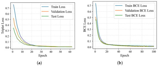
Figure 2.
Training dynamics of the DHGC framework: Loss plotted over epochs. The convergence of the training (blue) and validation (orange) loss curves demonstrates stable learning without overfitting. The test loss (green) is included for final model evaluation. (a) Triplet margin loss over training epochs. (b) Binary cross-entropy loss over training epochs.
The feature extractor, trained on 177,026 triplets, shows a quick drop in triplet margin loss during the first 20 epochs, then smoothly converges toward zero. Early stopping was triggered at epoch 64, with the model reaching training, validation, and test losses of 0.012, 0.014, and 0.011, respectively. This convergence suggests high embedding quality: the model achieved a test triplet accuracy of 99.6%, suggesting that the learned feature space effectively groups geologically similar windows while separating dissimilar ones. The close match among the training, validation, and test curves further suggests stable optimization and no overfitting.
The scoring model, trained on 354,052 feature pairs, shows a similarly steep initial reduction in BCE loss. By epoch 100, the model achieved a training BCE loss of 0.0122, a validation loss of 0.0101, and a test loss of 0.0125. Evaluation on the held-out test set yielded strong classification performance, with a Test Accuracy of 98.93%, F1-Score of 0.9894, and ROC-AUC of 0.9971. These results demonstrate that the scoring network functions as a highly reliable discriminator for the subsequent alignment phase.
To further validate the geological meaningfulness of the learned representations, we visualized the 32-dimensional embeddings of the first test log pair using t-SNE (Figure 3) [40]. The resulting latent space is highly structured. Windows with similar GR values, used here as a proxy for lithology, cluster tightly in the embedding space (Figure 3, right), indicating that the feature extractor captures distinct lithofacies. Importantly, these clusters are arranged along a smooth, continuous stratigraphic trajectory when colored by depth (Figure 3, left). This organization suggests that the model distinguishes geologically similar intervals occurring at different depths (e.g., shallow versus deep sands), providing the contextual fingerprints required for robust depth alignment.
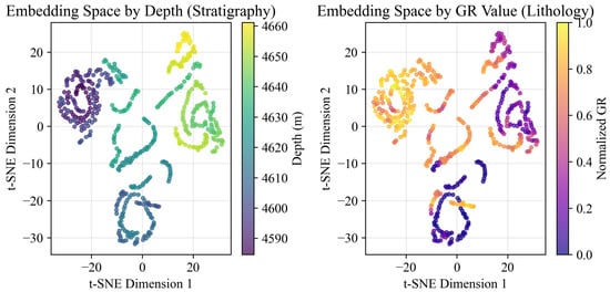
Figure 3.
t-SNE visualization of the learned embedding space for the first test log pair. Each point represents a 128-sample window, colored by depth (left) and normalized GR value (right).
3.2. Depth Alignment Performance
The alignment capability of the proposed DHGC framework was evaluated across 89 GR log pairs of varying lengths using Pearson correlation, Euclidean distance, and EMD. Figure 4 summarizes the distributions of these metrics.
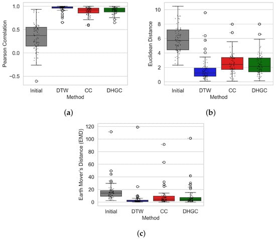
Figure 4.
Distribution of alignment performance metrics across 89 GR log pairs for the initial misalignment and after alignment using the proposed DHGC method. (a) Pearson Correlation; (b) Euclidean Distance; (c) Earth Mover’s Distance (EMD).
DHGC substantially improves alignment quality relative to the unaligned logs, raising the mean Pearson correlation from 0.35 to 0.91. This yields higher performance than CC (0.90) while remaining below DTW (0.96). Across the 89 pairs, DHGC achieves higher correlation than CC in 45 cases and outperforms DTW in 9 cases. Alignment improvement was observed in 88 of the 89 pairs; the one exception involved logs with no depth overlap.
A Friedman test [41] detected statistically significant differences among the three methods (). Post-hoc Wilcoxon signed-rank tests [42] showed that DTW achieved significantly higher correlations than both CC () and DHGC (). The difference between DHGC and CC was not statistically significant (), indicating that the proposed method delivers correlation performance comparable to CC while offering additional advantages.
Importantly, DHGC exhibits smaller interquartile ranges in both Euclidean distance and EMD compared to CC, indicating reduced variability and improved stability across log pairs. This enhanced consistency reflects the benefit of DHGC’s hierarchical structure, which is less sensitive to the global-shift assumption inherent to CC.
3.3. Visual Analysis of Log Alignment Performance
Visual inspection provides further insight into the behavior of each alignment approach. Figure 5 and Figure 6 present representative examples of successful and challenging cases.
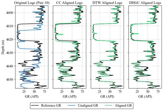
Figure 5.
Example of successful alignment (Pair 10). The columns show, from left to right: original logs, CC-aligned logs, DTW-aligned logs, and DHGC-aligned logs. The black line represents the reference GR log, the blue line represents the unaligned GR log, and the green line represents the aligned GR log using the corresponding method.
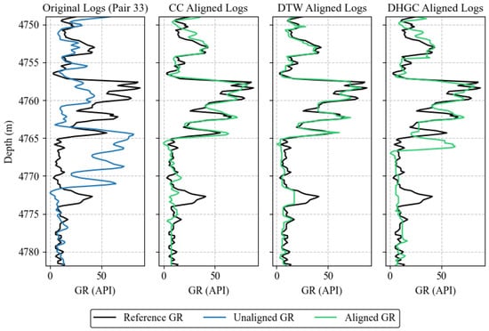
Figure 6.
Example of a challenging alignment case (Pair 33). Columns show, from left to right: original logs, CC-aligned logs, DTW-aligned logs, and DHGC-aligned logs. The black line denotes the reference GR log, the blue line the unaligned target log, and the green line the aligned log produced by each method.
3.3.1. Successful Alignment Case (Pair 10)
Pair 10 exhibits a clearly non-linear depth error, resulting in substantial initial misalignment (Pearson: 0.3428, Euclidean: 7.6734, EMD: 22.4972).
The proposed DHGC method achieves strong alignment performance in this challenging case (Pearson: 0.9558, Euclidean: 1.9912, EMD: 5.9503). Compared to CC, DHGC delivers improved correlation and reduced mismatch, while more effectively correcting the non-linear depth distortion. Qualitatively, DHGC preserves coherent stratigraphic structure across the interval, successfully aligning key features without introducing artificial flattening or distortion. For example, the distinct low GR interval at 4608–4621 m is correctly aligned with its counterpart, preserving the sharp boundary definition that is critical for seal capacity analysis.
In contrast, although DTW obtains the highest numerical alignment metrics (Pearson: 0.9920), it exhibits a critical artifact between 4640 m and 4645 m. In this interval, the DTW-aligned log displays a vertical line, indicating a constant-value anomaly caused by pathological warping (singularity) [43]. DTW stretches a single data point or a very narrow segment across an extended depth range, eliminating legitimate stratigraphic variation. While DTW achieves stronger numerical metrics, DHGC avoids these singularity artifacts and retains realistic stratigraphic variability.
3.3.2. Challenging Case (Pair 33): Failure Analysis and Mitigation
Pair 33 represents a rare failure case of the proposed DHGC framework, primarily due to the combination of extreme initial misalignment, rapid high-frequency geological variability, and the short effective length of the log segment under analysis. The target interval contains 217 samples (approximately 33 m), which is near the minimum length required for stable tie-point reconstruction, as discussed in Section 2.8.4. While the feature extractor remains robust, this configuration exposes limitations of window-based hierarchical alignment when applied to short log segments.
First, the logs in the 4755–4775 m interval are geologically equivalent but exhibit pronounced morphological differences. These discrepancies increase uncertainty in the scoring model, producing ambiguous match probabilities that propagate through the dynamic programming cost matrix. To address this, an uncertainty-aware rejection strategy can be applied, where intervals with match probabilities in a moderate range are flagged for manual review rather than forcibly aligned.
Second, the local depth shift in some intervals may approach or exceed the current window length, which surpasses the CNN’s trained invariance range. In such cases, a smaller window would not resolve the problem, as it provides insufficient context for feature matching. Instead, a larger window should be used initially to capture the displaced features and establish a coarse alignment. Once the gross misalignment is reduced, the window size can then be decreased for a secondary refinement pass, increasing tie-point density and improving the ability to track high-frequency depth variations. This adaptive, multi-scale approach allows DHGC to handle large local shifts while preserving fine-resolution alignment in short log segments.
Finally, the short log length limits tie-point density. The first and last 64 samples are influenced by endpoint extrapolation, and the remaining central portion is too short to produce a dense, well-distributed set of tie-points. This sparse coverage constrains the ability of linear interpolation to capture high-frequency variations accurately. Multi-scale fusion, which combines coarse and fine alignments with the coarse path constraining the fine search, can improve performance in such cases.
Based on this analysis, DHGC should be applied with caution to log segments shorter than 256 samples (i.e., twice the window size), particularly when the initial Pearson correlation is below 0.2. Such cases are rare in our dataset. Pair 33 is presented as a representative example of this failure mode, while the remaining log pairs were successfully aligned using DHGC.
3.4. Computational Efficiency
Figure 7 compares the computational cost of DTW, CC, and the proposed DHGC method. To provide quantitative context, the mean end-to-end runtimes per log pair were approximately 25.8 s for DTW, 0.62 s for CC, and 3.16 s for DHGC, while median runtimes were substantially lower at 2.7 s, 0.08 s, and 0.48 s, respectively. These statistics highlight that DHGC achieves a favorable balance between speed and robustness, offering geologically consistent alignments at a fraction of DTW’s computational cost, though slightly slower than CC.
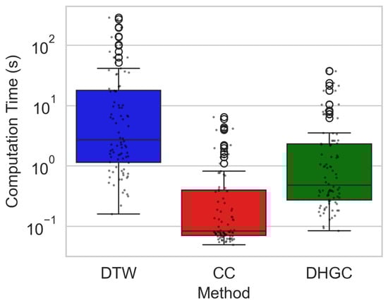
Figure 7.
End-to-end computation times (log scale) for DTW, CC, and DHGC across all log pairs. Each timing measurement represents the complete processing of one reference-target log pair, including data resampling, normalization, core alignment algorithm, signal reconstruction, and quality metric computation.
For DHGC, the reported runtime includes all processing stages executed within a single alignment call, including window extraction, feature embedding, cost-matrix construction, graph-based path optimization, and signal reconstruction. DTW and CC timings similarly reflect their complete alignment procedures.
DTW exhibits substantially higher runtimes due to sample-level dynamic programming with quadratic complexity, whereas CC is the fastest owing to its linear search over a fixed lag range. DHGC achieves this trade-off by operating at the window level and leveraging GPU-accelerated feature extraction.
All timing experiments were conducted on a Dell Precision 3591 workstation (Intel Core i7, 32 GB RAM, NVIDIA RTX A1000 GPU). CNN inference was executed on the GPU, while graph-based optimization was performed on the CPU. Training time for DHGC is excluded.
Overall, DHGC offers the balance among the evaluated methods. The model convergence analysis suggests that its deep learning components are stable, well-trained, and highly discriminative. Although DTW achieves the highest average correlation, it produces unrealistic warping artifacts and incurs high computational overhead. In contrast, DHGC outperforms CC in handling non-uniform geological shifts, showing significantly lower variability across Euclidean distance and EMD. Importantly, DHGC provides this geologically consistent alignment at a fraction of DTW’s computational cost. The combination of reliable accuracy, reduced variability, and high efficiency makes DHGC a practical and scalable solution for large-scale or near-real-time correlation workflows, particularly in settings where DTW is computationally prohibitive.
4. Discussion
The results presented herein demonstrate that the proposed DHGC framework outperforms standard CC in alignment accuracy while achieving a superior balance of geological consistency and computational efficiency compared to DTW. This performance is not accidental but stems from fundamental design choices regarding how the method handles the non-stationary complexities of well-log data.
4.1. Interpretation of Singularity-Free Alignment
A key qualitative difference between DHGC and standard DTW is the absence of singularity artifacts, i.e., vertical or horizontal path segments that collapse extended intervals onto individual samples (Figure 5). While the methodological constraints responsible for this behavior are described in Section 2.8.5, their effectiveness can be understood from a geological and optimization perspective.
At a conceptual level, DHGC discourages singularities by favoring globally coherent alignment patterns rather than locally optimal pointwise matches. The learned similarity scores reflect contextual agreement across depth intervals, making it unlikely for the optimizer to benefit from collapsing one interval onto many others. As a result, alignment paths that would be admissible under purely distance-based formulations are systematically deprioritized.
This behavior is further reinforced by the window-based representation, which implicitly encodes stratigraphic continuity. Because matching decisions are informed by interval-scale patterns rather than isolated samples, extreme stretch or squeeze operations become inconsistent with the learned representation of geological similarity. Singular alignments, therefore, lack semantic support in the embedding space, even if they might locally improve numerical correlation.
Finally, the constrained search space promotes physically plausible deformation by limiting how rapidly depth correspondence can change. Rather than allowing the optimizer to exploit pathological warping to fit noise, DHGC favors smooth depth-to-depth transitions that are consistent with expected stratigraphic relationships. This explains why DHGC may yield slightly lower peak correlation than unconstrained DTW while producing alignments that are more interpretable and geologically realistic.
Taken together, these effects explain why DHGC consistently avoids singularities without explicitly optimizing for their removal, maintaining stratigraphic continuity even in challenging intervals where unconstrained DTW tends to overfit.
4.2. Selection of Optimal Window Size
The window size serves as a critical hyperparameter that balances the trade-off between capturing high-frequency geological details and utilizing broader contextual information. We empirically evaluated four window sizes (32, 64, 128, and 256 samples) on the training dataset, as summarized in Table 2.
Table 2.
Performance metrics for varying window sizes on the test set. Bold values indicate the best performance for each metric. Train Time is measured per log pair.
The 128-sample window, corresponding to approximately 19.5 m, yielded the most robust results. This scale is geologically appropriate because wireline depth measurement errors typically range up to 10 m [6,28]. A window of approximately 20 m provides a sufficient receptive field to accommodate these deviations without losing context. In contrast, smaller windows (32 and 64 samples) lacked the contextual breadth to handle such errors effectively, while the 256-sample window (∼39 m) tended to over-smooth distinct features. Consequently, 128 samples was selected as the optimal window size for this study.
4.3. DHGC Performance vs. Traditional Methods
Standard CC is inherently limited by its assumption of a constant, linear global shift. Well-log data, however, is characterized by widespread non-linear depth shifts, including stretching and squeezing, as well as non-stationary noise, which is clearly seen in Figure 5. DHGC outperforms CC by explicitly accommodating these non-linearities. Its learned cost matrix captures local feature similarities directly from the data—as evidenced by the distinct stratigraphic and lithological clustering in the latent space (Figure 3)—and the graph-based optimization finds the optimal non-linear path through this matrix. This shifts the workflow from rigid linear assumptions to a flexible, data-driven alignment strategy capable of correcting complex distortions that CC misses.
While DTW achieves the highest mean correlation (0.96), it is slow and variable (see Figure 7), making it impractical for large-scale automated applications. DHGC addresses this limitation by providing near-DTW accuracy (0.91) with much faster inference, about quicker than DTW, and greater robustness than CC. This combination of speed and reliable non-linear alignment makes DHGC well-suited for automated subsurface characterization workflows.
4.4. Implications for Subsurface Characterization
The implications of this advancement extend beyond computational metrics. Accurate and efficient well-log alignment directly translates to more reliable geological interpretations and robust reservoir models, ultimately supporting more informed decision-making in hydrocarbon exploration and production [44]. This reliability is crucial for complex engineering challenges, ranging from hydrate risk mitigation [2] and fracture propagation analysis [3] to geothermal characterization [4]. By reducing reliance on subjective manual adjustments, the proposed DHGC framework provides a pathway toward fully automated, unbiased correlation workflows. This capability is particularly critical when managing the increasing volume of data from field-scale studies involving hundreds of wells, where manual alignment is no longer feasible.
4.5. Limitations
Despite its advantages, the current iteration of DHGC presents certain limitations derived from the failure analysis. First, in zones with rapid geological variation shorter than the window length, the fixed 128-sample window may smooth over fine-scale features. The hierarchical CNN architecture reduces sensitivity to short-wavelength structures, and the sparser tie-point density in these regions can lead to interpolation drift. Second, because the method utilizes window centers for tie-points, alignment precision naturally decreases in the first and last ∼10 m of the log sequence. These edge regions rely on extrapolated alignment, which may be less accurate than the central, fully constrained path. Third, as evidenced by Pair 33, the method requires log segments to exceed the window size (typically samples) and maintain at least 50% depth overlap; performance degrades significantly if these conditions are not met. Finally, while validated on GR logs, generalization to other log types, such as resistivity or density, will likely require retraining or transfer learning to account for differing noise profiles and feature scales.
4.6. Future Work
Future development of the DHGC framework will focus on four primary areas to address the aforementioned limitations. Research will investigate multi-scale architectures that utilize adaptive window sizes to improve sensitivity to short-wavelength deformations in high-frequency zones, directly addressing the smoothing issues observed in Pair 33. To enhance reliability in ambiguous, low-similarity regions, we aim to incorporate uncertainty quantification, transforming the output into a probabilistic alignment with confidence intervals. Furthermore, we plan to extend the framework to support multi-log fusion, allowing for the joint alignment of multiple curve types (e.g., GR, resistivity, and density) simultaneously to improve robustness. Finally, we will explore scalability adaptations, specifically for 3D multi-well correlation studies, alongside data-efficient transfer learning strategies to generalize the model to new basins with limited training data.
5. Conclusions
This study introduces the Deep Hierarchical Graph Correlator (DHGC), a framework for automated well-log depth alignment that integrates convolutional neural networks with constrained graph-based optimization. By combining learned similarity measures with physically motivated path constraints, the approach addresses key limitations of traditional methods, including the rigid linearity assumptions of CC and the unphysical artifacts and computational inefficiency commonly associated with unconstrained DTW.
Quantitative evaluation on 89 unseen log pairs suggests that DHGC achieves substantial improvements in alignment quality, increasing the mean Pearson correlation from 0.35 to 0.91 with a success rate of 98.9%. The method also yields an reduction in computation time relative to DTW (3.16 s versus 25.83 s per pair on average), indicating its suitability for larger datasets. Although DTW attains a slightly higher raw correlation (0.96), DHGC offers a more operationally consistent solution by enforcing slope constraints and employing a learned probabilistic cost matrix, which mitigates the singularity artifacts observed in unconstrained DTW. Visual inspection of the learned embedding space further suggests that the model captures both lithological characteristics and stratigraphic continuity.
The current implementation has limitations when applied to short log segments (<128 samples) and intervals characterized by extreme high-frequency heterogeneity, as observed in the failure analysis of Pair 33. Future work will explore multi-scale representations and uncertainty-aware formulations to improve robustness in such cases. In addition, although the framework is signal-agnostic, extending DHGC to joint multi-log alignment (e.g., resistivity and density) represents a natural direction for further development.
Overall, DHGC provides a promising step toward more automated and scalable well-log correlation. By balancing the flexibility of non-linear alignment with computational efficiency and geological plausibility, the framework has the potential to support large-scale subsurface characterization workflows.
Author Contributions
Conceptualization, S.A., K.F., A.Y. and K.W.; methodology, S.A.; software, S.A.; validation, S.A., K.F. and A.Y.; formal analysis, S.A.; investigation, S.A.; resources, K.W.; data curation, K.W.; writing—original draft preparation, S.A.; writing—review and editing, S.A., K.F., A.Y. and K.W.; visualization, S.A.; supervision, K.F., A.Y. and K.W. All authors have read and agreed to the published version of the manuscript.
Funding
This research received no external funding.
Institutional Review Board Statement
Not applicable.
Data Availability Statement
The data used in this study are subject to privacy and ethical restrictions. While some of the training data are publicly available, not all datasets can be shared due to confidentiality agreements and proprietary reasons. The code developed for this study is part of an ongoing PhD project and is not yet publicly available. It may be released in the future after the project is finished and with proper approvals.
Acknowledgments
The authors sincerely thank the Department of Geosciences at NTNU, the BRU21 Research Program, and Aker BP ASA, Oslo, for supporting this PhD project.
Conflicts of Interest
Author KjetilWesteng was employed by the company Aker BP ASA. The remaining authors declare that the research was conducted in the absence of any commercial or financial relationships that could be construed as a potential conflict of interest.
Abbreviations
The following abbreviations are used in this manuscript:
| BCE | Binary Cross-Entropy |
| CC | Cross-Correlation |
| CDTW | Constrained Dynamic Time Warping |
| CNN | Convolutional Neural Network |
| COW | Correlation Optimized Warping |
| DHGC | Deep Hierarchical Graph Correlator |
| DL | Deep Learning |
| DP | dynamic programming |
| DRL | Deep Reinforcement Learning |
| DTW | Dynamic Time Warping |
| EMD | Earth Mover’s Distance |
| EWL | Electric Wireline Logging |
| GR | Gamma-Ray |
| LAS | Log ASCII Standard |
| LWD | Logging While Drilling |
| ML | Machine Learning |
| ReLU | Rectified Linear Unit |
| RNN | Recurrent Neural Network |
References
- Torres Caceres, V.A.; Duffaut, K.; Yazidi, A.; Westad, F.O.; Johansen, Y.B. Automated well-log depth matching–1D convolutional neural networks vs. classic cross correlation. Petrophysics 2022, 63, 12–34. [Google Scholar] [CrossRef]
- Li, M.; Liu, J.; Xia, Y. Risk prediction of gas hydrate formation in the wellbore and subsea gathering system of deep-water turbidite reservoirs: Case analysis from the south China Sea. Reserv. Sci. 2025, 1, 52–72. [Google Scholar] [CrossRef]
- Cao, L.; Lv, M.; Li, C.; Sun, Q.; Wu, M.; Xu, C.; Dou, J. Effects of crosslinking agents and reservoir conditions on the propagation of fractures in coal reservoirs during hydraulic fracturing. Reserv. Sci. 2025, 1, 36–51. [Google Scholar] [CrossRef]
- Wang, F.; Kobina, F. The influence of geological factors and transmission fluids on the exploitation of reservoir geothermal resources: Factor discussion and mechanism analysis. Reserv. Sci. 2025, 1, 3–18. [Google Scholar] [CrossRef]
- Asquith, G.B.; Krygowski, D.; Gibson, C.R. Basic Well Log Analysis; American Association of Petroleum Geologists: Tulsa, OK, USA, 2004; Volume 16. [Google Scholar]
- Bolt, H. Wireline logging depth quality improvement: Methodology review and elastic-stretch correction. Petrophysics 2016, 57, 294–310. [Google Scholar]
- Bolt, H. Driller’s Depth Quality Improvement: Way-Point Methodology. Petrophysics 2017, 58, 564–575. [Google Scholar]
- Archie, G.E. Introduction to petrophysics of reservoir rocks. AAPG Bull. 1950, 34, 943–961. [Google Scholar] [CrossRef]
- Kerzner, M.G. A solution to the problem of automatic depth matching. In Proceedings of the SPWLA Annual Logging Symposium, SPWLA, New Orleans, LA, USA, 10–13 June 1984; p. SPWLA-1984. [Google Scholar]
- Ezenkwu, C.P.; Guntoro, J.; Starkey, A.; Vaziri, V.; Addario, M. Automated well-log pattern alignment and depth-matching techniques: An empirical review and recommendations. Petrophysics 2023, 64, 115–129. [Google Scholar] [CrossRef]
- Xu, C.; Fu, L.; Lin, T.; Li, W.; Alzayer, Y.; Al Ibrahim, Z. Automatic depth shifting by identifying and matching events on well logs. Petrophysics 2024, 65, 246–255. [Google Scholar] [CrossRef]
- Liang, L.; Shan, T.; Li, J.; Lei, T. A Multi-Scale Cross-Correlation Based Method Enables Automatic Well Log Depth Matching. In Proceedings of the International Petroleum Technology Conference, IPTC, Kuala Lumpur, Malaysia, 18–20 February 2025; p. D012S004R008. [Google Scholar]
- Zimmermann, T.; Liang, L.; Zeroug, S. Machine-learning-based automatic well-log depth matching. Petrophysics 2018, 59, 863–872. [Google Scholar] [CrossRef]
- Le, T.; Liang, L.; Zimmermann, T.; Zeroug, S.; Heliot, D. A machine-learning framework for automating well-log depth matching. Petrophysics 2019, 60, 585–595. [Google Scholar] [CrossRef]
- Acharya, S.; Fabian, K. Dynamic Depth Alignment of Well-bore Measurements Using Machine Learning. In Proceedings of the 84th EAGE Annual Conference & Exhibition, European Association of Geoscientists & Engineers, Vienna, Austria, 5–8 June 2023; Volume 2023, pp. 1–5. [Google Scholar]
- Acharya, S.; Fabian, K.; Yazidi, A.; Westeng, K. Automated Depth Alignment of Well Logs Using Siamese Neural Networks. In Proceedings of the SPWLA Annual Logging Symposium, SPWLA, Dubai, United Arab Emirates, 17–21 May 2025; p. D041S010R002. [Google Scholar]
- Caceres, V.A.T.; Duffaut, K.; Yazidi, A.; Westad, F.; Johansen, Y.B. Automated well log depth matching: Late fusion multimodal deep learning. Geophys. Prospect. 2023, 72, 155–182. [Google Scholar] [CrossRef]
- Meng, F.; Fan, X.; Chen, S.; Ye, Y.; Jiang, H.; Pan, W.; Wu, F.; Zhang, H.; Chen, Y.; Semnani, A. Automatic well-log depth shift with multilevel wavelet decomposition network and dynamic time warping. Geoenergy Sci. Eng. 2025, 246, 213583. [Google Scholar] [CrossRef]
- Acharya, S.; Fabian, K. Unsupervised Machine Learning for Well Log Depth Alignment. In Proceedings of the International Conference on Offshore Mechanics and Arctic Engineering, Singapore, 9–14 June 2024; American Society of Mechanical Engineers: New York, NY, USA, 2024; Volume 87868, p. V008T11A019. [Google Scholar]
- Acharya, S.; Fabian, K.; Westeng, K. Comparison of Supervised and Unsupervised Machine Learning for Well-Log Depth Alignment. In Proceedings of the SPE/IADC Drilling Conference and Exhibition, SPE, Stavanger, Norway, 4–6 March 2025; p. D022S007R002. [Google Scholar]
- Xiong, W.; Lizhi, X.; Jiangru, Y.; Wenzheng, Y. Automatic depth matching method of well log based on deep reinforcement learning. Pet. Explor. Dev. 2024, 51, 634–646. [Google Scholar] [CrossRef]
- Bittar, M.; Wang, S.; Wu, X.; Chen, J. Multiple well-log depth matching using deep q-learning. Petrophysics 2021, 62, 353–361. [Google Scholar] [CrossRef]
- Zhang, W.; Gu, X.; Tang, L.; Yin, Y.; Liu, D.; Zhang, Y. Application of machine learning, deep learning and optimization algorithms in geoengineering and geoscience: Comprehensive review and future challenge. Gondwana Res. 2022, 109, 1–17. [Google Scholar] [CrossRef]
- Sakoe, H.; Chiba, S. Dynamic programming algorithm optimization for spoken word recognition. IEEE Trans. Acoust. Speech Signal Process. 2003, 26, 43–49. [Google Scholar] [CrossRef]
- Berndt, D.J.; Clifford, J. Advances in Knowledge Discovery and Data Mining; American Association for Artificial Intelligence: Menlo Park, CA, USA, 1996; pp. 229–248. [Google Scholar]
- Alzubaidi, L.; Zhang, J.; Humaidi, A.J.; Al-Dujaili, A.; Duan, Y.; Al-Shamma, O.; Santamaría, J.; Fadhel, M.A.; Al-Amidie, M.; Farhan, L. Review of deep learning: Concepts, CNN architectures, challenges, applications, future directions. J. Big Data 2021, 8, 53. [Google Scholar] [CrossRef] [PubMed]
- Acharya, S.; Fabian, K. Machine learning and explainable AI for predicting missing well log data with uncertainty analysis: A case study in the Norwegian North Sea. In Proceedings of the SEG/AAPG International Meeting for Applied Geoscience & Energy, SEG, Houston, TX, USA, 26–29 August 2024. SEG-2024-4101553. [Google Scholar]
- Theys, P.P. Log Data Acquisition and Quality Control; Editions Technip: Paris, France, 1999. [Google Scholar]
- Agarap, A.F. Deep Learning using Rectified Linear Units (ReLU). arXiv 2018, arXiv:1803.08375. [Google Scholar]
- Scherer, D.; Müller, A.; Behnke, S. Evaluation of pooling operations in convolutional architectures for object recognition. In Proceedings of the International Conference on Artificial Neural Networks, Thessaloniki, Greece, 15–18 September 2020; Springer: Berlin/Heidelberg, Germany, 2010; pp. 92–101. [Google Scholar]
- Van der Walt, S.; Schönberger, J.L.; Nunez-Iglesias, J.; Boulogne, F.; Warner, J.D.; Yager, N.; Gouillart, E.; Yu, T. scikit-image: Image processing in Python. PeerJ 2014, 2, e453. [Google Scholar] [CrossRef] [PubMed]
- Dijkstra, E.W. A note on two problems in connexion with graphs. In Edsger Wybe Dijkstra: His Life, Work, and Legacy; ACM Digital Library: New York, NY, USA, 2022; pp. 287–290. [Google Scholar]
- Schlumberger Limited. Log Interpretation Principles/Applications; Schlumberger Educational Services: Houston, TX, USA, 1991. [Google Scholar]
- Hoffer, E.; Ailon, N. Deep metric learning using triplet network. In Proceedings of the International Workshop on Similarity-Based Pattern Recognition, Copenhagen, Denmark, 12–14 October 2015; Springer: Berlin/Heidelberg, Germany, 2015; pp. 84–92. [Google Scholar]
- Fawcett, T. An introduction to ROC analysis. Pattern Recognit. Lett. 2006, 27, 861–874. [Google Scholar] [CrossRef]
- Pearson, K., VII. Mathematical contributions to the theory of evolution—III. Regression, heredity, and panmixia. Philos. Trans. R. Soc. Lond. Ser. A Contain. Pap. A Math. Phys. Character 1896, 187, 253–318. [Google Scholar] [CrossRef]
- Bishop, C.M.; Nasrabadi, N.M. Pattern Recognition and Machine Learning; Springer: Berlin/Heidelberg, Germany, 2006; Volume 4. [Google Scholar]
- Rubner, Y.; Tomasi, C.; Guibas, L.J. The earth mover’s distance as a metric for image retrieval. Int. J. Comput. Vis. 2000, 40, 99–121. [Google Scholar] [CrossRef]
- Oppenheim, A.V. Discrete-Time Signal Processing; Pearson Education India: New Delhi, India, 1999. [Google Scholar]
- Maaten, L.V.D.; Hinton, G. Visualizing data using t-SNE. J. Mach. Learn. Res. 2008, 9, 2579–2605. [Google Scholar]
- Friedman, M. The use of ranks to avoid the assumption of normality implicit in the analysis of variance. J. Am. Stat. Assoc. 1937, 32, 675–701. [Google Scholar] [CrossRef]
- Wilcoxon, F. Individual comparisons by ranking methods. In Breakthroughs in Statistics: Methodology and Distribution; Springer: New York, NY, USA, 1992; pp. 196–202. [Google Scholar]
- Keogh, E.J.; Pazzani, M.J. Derivative Dynamic Time Warping. In Proceedings of the 2001 SIAM International Conference on Data Mining (SDM), Chicago, IL, USA, 5–7 April 2001; pp. 1–11. [Google Scholar] [CrossRef]
- Misra, S.; Li, H.; He, J. Machine Learning for Subsurface Characterization; Gulf Professional Publishing: Houston, TX, USA, 2019. [Google Scholar]
Disclaimer/Publisher’s Note: The statements, opinions and data contained in all publications are solely those of the individual author(s) and contributor(s) and not of MDPI and/or the editor(s). MDPI and/or the editor(s) disclaim responsibility for any injury to people or property resulting from any ideas, methods, instructions or products referred to in the content. |
© 2025 by the authors. Licensee MDPI, Basel, Switzerland. This article is an open access article distributed under the terms and conditions of the Creative Commons Attribution (CC BY) license.