Formation Control of Multiple UUVs Based on GRU-KF with Communication Packet Loss

Abstract

In response to the problem of decreased collaborative control performance in underwater unmanned vehicles (UUVs) with communication packet loss, a GRU-KF method for multi-UUV control that integrates a gated recurrent unit (GRU) and a Kalman filter (KF) is proposed. First, a UUV feedback linearization model and a current model are established, and a multi-UUV controller-based leader–follower method is designed, using a neural network-based radial basis function (RBF) to counteract the uncertainty effects in the model. For scenarios involving packet loss in multi-UUV collaborative communication, the GRU network extracts historical temporal features to enhance the system’s adaptability to communication uncertainties, while the KF performs state estimation and error correction. The simulation results show that, compared to compensation by the GRU network, the proposed method significantly reduces the jitter level and convergence time of errors, enabling the formation to exhibit good robustness and accuracy in communication packet loss scenarios.

1. Introduction

Unmanned underwater vehicles (UUVs) serve as indispensable autonomous platforms for ocean exploration, performing tasks including marine resource sampling [1,2], subsea pipeline inspection [3,4,5], and military reconnaissance [6,7] without human intervention. Their operational scope remains constrained by endurance and payload limitations, driving significant research interest in cooperative UUV formations.

To achieve the cooperative operation of UUV formations, information exchange between UUVs needs to be carried out through underwater communication. Due to the long transmission distance and strong penetrability, hydroacoustic communication is the most widely used communication method at present. However, due to the specific characteristics of the underwater environment, hydroacoustic communication has certain limitations: the bandwidth of hydroacoustic communication is limited and susceptible to interference, which can cause time delays and packet loss during information transmission between UUVs [8]. Yan et al. constructed a discrete-time control architecture based on the virtual leader and established a sufficient condition for the convergence of the system based on Shuler’s theory [9]; Chen and Guo proposed an AUV formation-control algorithm based on consistency theory and the leader–follower method, and introduced a hybrid communication topology to adapt to the control of large formations [10]; Li et al. categorized communication into effective and ineffective categories through delay limitation, and designed an AUV formation-control method based on the switching of communication topology to address the problem of ineffective communication [11]; Jiang et al. designed a formation-control protocol with deterministic switching signals to solve the problem of weak communication [12]; Kuniyoshi et al. designed a sequential inter-carrier interference countermeasure to improve the channel transfer function [13]; Yan and Pan considered communication delay to be a specific function with upper and lower bounds, and proposed three coordinated control protocols to achieve UUV formation control [14]. Kiran et al. used artificial intelligence and reinforcement learning to optimize underwater communication protocols, and demonstrated the improved efficiency of AI-assisted communication compared to traditional methods by employing experimental design metrics [15]; Yan et al. designed a state message buffer to synchronize asynchronous messages with communication delays [16]; Cai et al. applied event-triggered leader–follower communication mechanisms to a formation-control model that reduces the number of unnecessary communications between multiple UUVs [17], but has strict requirements regarding the triggering conditions and constraints; and Tang et al. introduced hierarchical reinforcement learning to improve the communication rate of a maritime system through reinforcement learning [18]. Determining how to achieve stable and efficient UUV formation control with underwater communication constraints is a key direction in current UUV formation research.

Although significant progress has been made in UUV formation control under communication constraints, several critical challenges persist: first, existing studies often employ oversimplified multi-UUV models, inadequately accounting for model uncertainty and external disturbances; second, research on communication constraints predominantly focuses on time delay issues, while information gaps caused by communication packet loss remain insufficiently explored.

On this basis, this paper proposes a GRU-KF-based UUV formation-control method for the problem of communication packet loss in the cooperative control of UUV formations. The main contributions of this study are as follows:

(1)

In order to achieve the cooperative control of UUV formations, a backstepping sliding mode controller based on the leader–follower method is designed by combining the relative position constraints of the leader and the follower.

(2)

In order to solve the problem of communication packet loss, a GRU network is utilized to predict the time series of the leader’s trajectory; then, a Kalman filter is introduced, and the predicted value of the GRU network is used as the measured value of the state in the Kalman filtering algorithm to update the leader’s state in real time. This method can optimize the control performance of the UUV formation under the influence of communication packet loss and reduce the control errors caused by external environmental interference.

2. UUV Model

Mathematical models of UUVs represent the basis for studying their motion characteristics and control problems, which directly affect the accuracy and performance of their control algorithms. In practical applications, UUVs are usually underactuated, and to reduce model complexity and align with the actual mission requirements, we consider the rolling of UUVs to be self-stabilizing [19]. Given the prevalence of ocean currents in underwater environments, establishing a current disturbance model is essential to investigating their impact on UUV motion control and enhancing operational precision.

2.1. UUV Linearization Model

In order to study the motion of UUVs, it is necessary to establish a coordinate system that can accurately describe changes in UUV state variables; in this study, an inertial coordinate system $\left\{E\right\}$ and a carrier coordinate system $\left\{B\right\}$ are established, as shown in Figure 1.

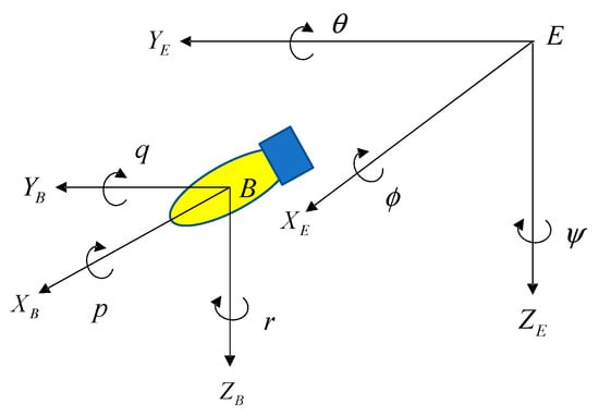
Figure 1. Coordinate system.

The inertial coordinate system takes the earth or the seabed as the reference point and is a fixed global coordinate system. The axes of this coordinate system are defined as follows: $X_E$ points to the north; $Y_E$ is on the horizontal plane, coplanar and perpendicular to $X_E$, and points to the east; and $Z_E$ points vertically downward.

The carrier coordinate system generally takes the center of mass of the UUV as the origin, and the coordinate axes are defined as follows: $X_B$ is oriented along the yaw direction of the UUV, pointing forward; $Y_B$ is oriented along the starboard direction, pointing to the right side; and $Z_B$ points vertically downward.

$\eta ={[xyz\theta \psi ]}^{\mathrm{T}}\in R^3\times S^2$ denotes the attitude vector in the fixed coordinate system, $\nu ={[uvwqr]}^{\mathrm{T}}\in R^5$ denotes the velocity vector in the carrier coordinate system, and $T={[XYZMN]}^{\mathrm{T}}\in R^6$ denotes the force and moment in the carrier coordinate system.

Combining the UUV kinematics and dynamics models, the vector expression of the nonlinear model of the UUV can be obtained as follows:

$$\begin{array}{l}\hfill \dot{\eta }=J(\eta )v\hfill \\ \hfill M_R\dot{v}+M_A\dot{v}+C_R(v)v+Y(v)+g(\eta )=T+\omega \hfill \end{array}$$

(1)

where $\omega$ is the external perturbation of the UUV, $J(\eta )$ is the coordinate system transformation matrix, $M_R$ and $M_A$ are the rigid-body inertia matrix and the additional mass matrix, $C_R(v)$ is the Coriolis matrix, $Y(v)$ is the fluid damping matrix, and $g(\eta )$ is the vector of restoring force exerted by gravity and buoyancy simultaneously.

To achieve feedback linearization of the nonlinear mathematical model of the UUV, the second-order integral model is obtained as follows:

$$\begin{array}{l}{\dot{z}}_1=z_2\\ {\dot{z}}_2=u\end{array}$$

(2)

where $z_1$ is the position information of the UUV after coordinate transformation, $z_2$ is its velocity information, and $u$ is its control input.

2.2. Current Model

In an actual marine environment, ocean currents are common and affected by many factors. During motion control, vehicles experience not only actuator inputs but also hydrodynamic disturbances from currents. Current forces have hydrodynamic effects on vehicles, including perturbation forces on the hull and perturbation torques. These forces and torques affect the kinematic performance of the UUV. Therefore, the effect of current disturbances needs to be considered when designing UUV controllers.

A current is a vector with magnitude and direction, and the mathematical model of a current in an inertial coordinate system is

$$d_{cur}^E=\left[\begin{array}{c}{u}_c^E\\ v_c^E\\ w_c^E\end{array}\right]$$

(3)

where $u_c^E$ is the northward velocity of the current in the inertial coordinate system, $v_c^E$ is its eastward velocity, and $w_c^E$ is its vertical velocity.

The expression of the current in the carrier coordinate system is given by

$$\left[\begin{array}{c}{u}_c^B\\ v_c^B\\ w_c^B\end{array}\right]=J_v{({\eta }_r)}^T\left[\begin{array}{c}{u}_c^E\\ v_c^E\\ w_c^E\end{array}\right]$$

(4)

where $u_c^B$ is the northward velocity of the current in the carrier coordinate system, $v_c^B$ is its eastward velocity, and $w_c^B$ is its vertical velocity.

The relative velocity of the UUV with respect to the current is

$$v_{relative}=\left[\begin{array}{c}{u}_r\\ v_r\\ w_r\end{array}\right]=\left[\begin{array}{c}u-u_{\mathrm{c}}^B\\ v-v_c^B\\ w-w_c^B\end{array}\right]$$

(5)

3. UUV Controller Design

In this section, a multi-UUV formation controller is designed based on the leader–follower method, where the follower UUVs can dynamically adjust according to the state information of the leader UUV to maintain the preset formation. In addition, we consider that in practical applications, dynamics models of UUVs often have uncertainties, such as changes in hydrodynamic coefficients and uncertain parts of the models. Therefore, we also design a backstepping sliding mode controller [20] based on an RBF neural network to offset the effect of model uncertainty on UUV control.

3.1. Design of UUV Controller Based on Backstepping Sliding Mode

In practical applications, there is uncertainty in UUV models; the UUV model with uncertainty and current disturbance based on Equation (2) is

$$\begin{array}{c}{\dot{z}}_1=z_2\\ {\dot{z}}_2+\Delta =u+d_{cur}(t)\end{array}$$

(6)

where $\Delta$ is the model uncertainty constraint, and $d_{cur}(t)$ is the current disturbance.

Assuming the position and attitude information of the leader $z_1^L={\eta }_L$, the information on the desired position and attitude of the ith follower is given as $z_{1d}^{Fi}=z_1^L+d_i$. Define the position and attitude tracking error as

$$\begin{array}{cc}\hfill e_1^i& =z_{1d}^{Fi}-z_1^{Fi}\hfill \\ & =z_1^L+d_i-z_1^{Fi}\hfill \end{array}$$

(7)

Define the Lyapunov function [21] as

$$V_1={\displaystyle \frac{1}{2}}{e}_1^{i\hspace{0.17em}2}$$

(8)

The differentiation of V₁ in Equation (8) can be obtained as follows:

$$\begin{array}{cc}\hfill {\dot{V}}_1& =e_1^i{\dot{e}}_1^i\hfill \\ & =e_1^i({\dot{z}}_{1d}^{Fi}-z_2^{Fi})\hfill \\ & =e_1^i(z_2^L+d{v}_i-z_2^{Fi})\hfill \end{array}$$

(9)

From Equation (9), when $z_2^{Fi}$ tends to $z_2^L+d{v}_i+c_1^i{e}_1^i$ ($c_1^i$ is a constant greater than 0), ${\dot{V}}_1=-c_1^i{e}_1^{i\hspace{0.17em}2}\le 0$. When ${\dot{V}}_1\equiv 0$, $e_1^i\equiv 0$, the closed-loop system is asymptotically stabilized.

Let $z_{2d}^{Fi}=z_2^L+d{v}_i+c_1^i{e}_1^i$. Then the next control objective is

$$e_2^i=z_{2d}^{Fi}-z_2^{Fi}$$

(10)

Replace $z_{2d}^{Fi}$ in Equation (10) with $z_2^L+d{v}_i+c_1^i{e}_1^i$, while ${\dot{e}}_1^i=z_2^L+d{v}_i-z_2^{Fi}$

$${\dot{e}}_1^i=e_2^i-c_1^i{e}_1^i$$

(11)

Define the sliding mode as

$${\sigma }^i=k_1^i{e}_1^i+e_2^i$$

(12)

where $k_1^i$ is a constant greater than 0. Then,

$${\sigma }^i=(k_1^i+c_1^i)e_1^i+{\dot{e}}_1^i$$

(13)

Define the Lyapunov function as

$$V_2=V_1+{\displaystyle \frac{1}{2}}{\sigma }^{i\hspace{0.17em}2}$$

(14)

Derive V₂ and substitute Equation (11) into it as follows:

$$\begin{array}{cc}\hfill {\dot{V}}_2& ={\dot{V}}_1+{\sigma }^i{\dot{\sigma }}^i\hfill \\ & =e_1^i(e_2^i-c_1^i{e}_1^i)+{\sigma }^i(k_1^i{\dot{e}}_1^i+{\dot{e}}_2^i)\hfill \\ & =e_1^i{e}_2^i-c_1^i{e}_1^{i2}+{\sigma }^i(k_1^i(e_2^i-c_1^i{e}_1^i)+{\dot{z}}_{2d}^{Fi}-{\dot{z}}_2^{Fi})\hfill \\ & =e_1^i{e}_2^i-c_1{e_1}^2+{\sigma }^i(k_1^i(e_2^i-c_1^i{e}_1^i)+{\dot{z}}_{2d}^{Fi}-u^i-d_{cur}^i(t)+{\Delta }^i)\hfill \end{array}$$

(15)

To ensure that the derivative of the Lyapunov function is negative definite, the control law is designed as follows:

$$u^i=k_1^i(e_2^i-c_1^i{e}_1^i)+{\dot{z}}_{2d}^{Fi}+{\eta }^i\mathrm{sgn}({\sigma }^i)+{\Delta }^i+e_1^i$$

(16)

where ${\eta }^i$ is a constant greater than 0, and $\mathrm{sgn}(\cdot )$ is the sign function.

Substituting Equation (16) into Equation (15), it can be determined that

$${\dot{V}}_2=-c_1^i{e}_1^{i\hspace{0.17em}2}-k_1^i{e}_1^{i\hspace{0.17em}2}-{\eta }^i\left|{\sigma }^i\right|-{\sigma }^i{d}_{cur}^i(t)$$

(17)

By taking the values of $c_1^i$, $k_1^i$, and ${\eta }^i$, we can obtain ${\eta }^i\ge D^i$ and thus ensure that ${\dot{V}}_2\le 0$, so the controller designed in this section is stable.

3.2. Design of UUV Controller Based on RBF Neural Network

To address the uncertainty in the dynamics model, the nonlinear fitting ability of the RBF neural network is utilized to estimate and compensate for the model uncertainty term [22]. RBF neural networks typically consist of an input layer, a hidden layer, and an output layer. The input layer receives input signals and transmits them to the hidden layer. In this study, the hidden layer uses a Gaussian function as the activation function, which is expressed as follows [23]:

$$\begin{array}{cc}{h}_j=\exp (-{\displaystyle \frac{{‖x-c_j‖}^2}{2{b_j}^2}})& j=1,2,\dots p\end{array}$$

(18)

$$f(x)=W^{\ast T}h(x)+\epsilon$$

(19)

where $h={\left[h_j\right]}^T$ is the output of the Gaussian function; $p$ is the number of nodes in the hidden layer of the RBF neural network; $W^{\ast }$ is the weight of the RBF neural network; and $\epsilon$ is the approximation error of the RBF network.

The input of RBF neural network is taken as $x^i={\left[\begin{array}{cc}{e}_1^i& e_2^i\end{array}\right]}^T$, and the output of RBF neural network is

$${\widehat{f}}^i(x)={\widehat{W}}^{i\hspace{0.17em}T}h(x^i)$$

(20)

where ${\widehat{W}}^i$ is the estimated weight of the RBF network.

Replacing the model uncertainty term ${\Delta }^i$ in the controller with the output of the RBF neural network, the designed control law can be written as

$$u^i=k_1^i(e_2^i-c_1^i{e}_1^i)+{\dot{z}}_{2d}^{Fi}+{\eta }^i\mathrm{sgn}({\sigma }^i)+{\widehat{f}}^i(x)+e_1^i$$

(21)

Substitute the controller into Equation (15) as follows:

$${\dot{V}}_2=-c_1^i{e}_1^{i\hspace{0.17em}2}-k_1^i{e}_1^{i\hspace{0.17em}2}-{\eta }^i\left|{\sigma }^i\right|-{\sigma }^i{d}_{cur}^i(t)+{\sigma }^i(-{\widehat{f}}^i(x)+{\Delta }^i)$$

(22)

Define ${\tilde{f}}^i(x)$ as follows:

$$\begin{array}{cc}\hfill {\tilde{f}}^i(x)& =f^i(x)-{\widehat{f}}^i(x)\hfill \\ & =W^{\ast iT}h(x^i)+{\epsilon }^i-{\widehat{W}}^{iT}h(x^i)\hfill \\ & ={\tilde{W}}^{iT}h(x^i)+{\epsilon }^i\hfill \end{array}$$

(23)

where ${\tilde{W}}^i=W^{\ast i}-{\widehat{W}}^i$.

Define the Lyapunov function as

$$V_3=V_1+{\displaystyle \frac{1}{2}}{\sigma }^{i2}+{\displaystyle \frac{1}{2}}{\gamma }^i{\tilde{W}}^{iT}{\tilde{W}}^i$$

(24)

where ${\gamma }^i$ is a constant greater than 0.

Derive V₃ as follows:

$$\begin{array}{cc}\hfill {\dot{V}}_3& ={\dot{V}}_1+{\sigma }^i{\dot{\sigma }}^i+{\gamma }^i{\tilde{W}}^{iT}{\dot{\tilde{W}}}^i\hfill \\ & =e_1^i{e}_2^i-c_1^i{e}_1^{i\hspace{0.17em}2}+{\sigma }^i(k_1^i(e_2^i-c_1^i{e}_1^i)+{\dot{z}}_{2d}^{Fi}-u^i-d_{cur}^i(t)+{\Delta }^i)-{\gamma }^i{\tilde{W}}^{iT}{\dot{\widehat{W}}}^i\hfill \end{array}$$

(25)

Substituting the control law into Equation (25) and ${\Delta }^i=f^i(x)$, we can obtain

$$\begin{array}{cc}\hfill {\dot{V}}_3& =-c_1^i{e}_1^{i\hspace{0.17em}2}-k_1^i{e}_1^{i\hspace{0.17em}2}+{\sigma }^i(-{\eta }^i\mathrm{sgn}({\sigma }^i)-d_{cur}^i(t)-{\widehat{f}}^i(x)+f^i(x))-{\gamma }^i{\tilde{W}}^{iT}{\dot{\widehat{W}}}^i\hfill \\ & =-c_1^i{e}_1^{i\hspace{0.17em}2}-k_1^i{e}_1^{i\hspace{0.17em}2}+{\sigma }^i(-{\eta }^i\mathrm{sgn}({\sigma }^i)-d_{cur}^i(t)+{\tilde{W}}^{iT}{h}^i(x)+{\epsilon }^i)-{\gamma }^i{\tilde{W}}^{iT}{\dot{\widehat{W}}}^i\hfill \\ & =-c_1^i{e}_1^{i\hspace{0.17em}2}-k_1^i{e}_1^{i\hspace{0.17em}2}+{\sigma }^i(-{\eta }^i\mathrm{sgn}({\sigma }^i)-d_{cur}^i(t)+{\epsilon }^i)+{\tilde{W}}^{iT}({\sigma }^i{h}^i(x)-{\gamma }^i{\dot{\widehat{W}}}^i)\hfill \end{array}$$

(26)

The design of the adaptive law is

$${\dot{\widehat{W}}}^i={\displaystyle \frac{h^i(x){\sigma }^i}{{\gamma }^i}}$$

(27)

Then,

$${\dot{V}}_3=-c_1^i{e}_1^{i\hspace{0.17em}2}-k_1^i{e}_1^{i\hspace{0.17em}2}-{\eta }^i\left|{\sigma }^i\right|-(d_{cur}^i(t)-{\epsilon }^i){\sigma }^i$$

(28)

Since the approximation error ${\epsilon }^i$ can be limited a small-enough value, ${\dot{V}}_3\le 0$ can be determined by taking ${\eta }^i\ge (d_{cur}^i(t)-{\epsilon }^i)$.

Assume that ${\eta }_0^i>0$, ${\eta }^i\ge {\eta }_0^i+d_{cur}^i(t)-{\epsilon }^i$; then,

$${\dot{V}}_3\le -c_1^i{e}_1^{i\hspace{0.17em}2}-k_1^i{e}_1^{i\hspace{0.17em}2}-{\eta }_0^i\left|{\sigma }^i\right|\le 0$$

(29)

Since $V_3\ge 0$, ${\dot{V}}_3\le 0$, ${\sigma }^i$, and ${\tilde{W}}^i$ are bounded. When the time tends to infinity, ${\sigma }^i$ tends to 0, which makes $e_1^i$ and $e_2^i$ tend to 0. Therefore, the designed controller is stable and convergent.

3.3. Design of UUV Formation Controller-Based Leader–Follower Method

The leader–follower method designates one UUV as the leader, responsible for trajectory planning and transmitting navigation states (position, attitude, and velocity) to follower vehicles within the formation [24]. Followers execute trajectory-tracking control based on received data to maintain preset relative positions, thereby achieving cooperative formation control. A schematic diagram of the leader–follower method is shown in Figure 2.

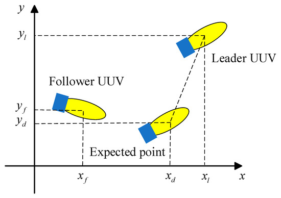
Figure 2. The leader–follower method.

In this section, we implement a leader-based UUV triangular formation, which requires the ability to maintain the formation in 3D space, as shown in Figure 3.

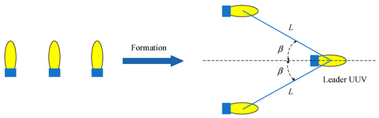
Figure 3. Leader–follower formation.

Here, L is the distance between the leader and the follower, and $\beta$ is the attitude angle of the formation.

Taking the spiral dive motion as an example, the constraint method designed in this study is as follows:

$$\begin{array}{l}\left\{\begin{array}{c}{\eta }_L+d_1={\eta }_{F1}\\ {\eta }_L+d_2={\eta }_{F2}\end{array}\right.\\ \left\{\begin{array}{c}{\dot{\eta }}_L+d{v}_1={\dot{\eta }}_{F1}\\ {\dot{\eta }}_L+d{v}_2={\dot{\eta }}_{F2}\end{array}\right.\end{array}$$

(30)

where ${\eta }_L$ is the position and attitude information of the leader, ${\dot{\eta }}_L$ is the velocity information of the leader in the inertial coordinate system, ${\eta }_{F1}$ and ${\eta }_{F2}$ are the position and attitude information of the two followers, ${\dot{\eta }}_{F1}$ and ${\dot{\eta }}_{F2}$ are the velocity information of the two followers in the inertial coordinate system, $d_1$ and $d_2$ are the corresponding attitude offsets, and $d{v}_1$ and $d{v}_2$ are the corresponding velocity offsets in the inertial coordinate system. The expressions of $d_1$, $d_2$, $d{v}_1$, and $d{v}_2$ are as follows:

$$\begin{array}{l}\left\{\begin{array}{c}{d}_1=\left[\begin{array}{lllll}-L\cos (\psi -\beta )\hfill & -L\sin (\psi -\beta )\hfill & 0\hfill & 0\hfill & \arctan (-L\cos \beta ,R-L\sin \beta )\hfill \end{array}\right]\\ d_2=\left[\begin{array}{lllll}-L\cos (\psi +\beta )\hfill & -L\sin (\psi +\beta )\hfill & 0\hfill & 0\hfill & \arctan (-L\cos \beta ,R+L\sin \beta )\hfill \end{array}\right]\end{array}\right.\\ \left\{\begin{array}{c}d{v}_1=\left[\begin{array}{lllll}L\sin (\psi -\beta )\ast \dot{\psi }\hfill & -L\cos (\psi -\beta )\ast \dot{\psi }\hfill & 0\hfill & 0\hfill & 0\hfill \end{array}\right]\\ d{v}_2=\left[\begin{array}{lllll}L\sin (\psi +\beta )\ast \dot{\psi }\hfill & -L\cos (\psi +\beta )\ast \dot{\psi }\hfill & 0\hfill & 0\hfill & 0\hfill \end{array}\right]\end{array}\right.\end{array}$$

(31)

where R is the radius of gyration of the leader in a spiral dive motion, and $\dot{\psi }$ is the yaw angular velocity of the UUV in the inertial coordinate system. Due to the difference in the radius of gyration, the expected yaw angles of the leader and the follower are not the same when the UUV formation is in a spiral dive motion with a fixed deviation.

4. Design of GRU-KF-Based Formation Controller with Communication Packet Loss

4.1. Analysis of Formation Control with Communication Packet Loss

In UUV formation control, instability in hydroacoustic communication links can cause communication packet loss—failure to transmit the leader’s state information to followers. The main reasons for communication packet loss include the attenuation of underwater acoustic signals and environmental interference. When communication packet loss occurs, followers lack access to the leader’s state data for extended periods, resulting in accumulated trajectory prediction errors that ultimately compromise formation integrity.

The main impacts of communication packet loss are as follows: First, communication packet loss renders the follower unable to obtain the state information of the leader in real time, which leads to the error accumulation and thus affects the trajectory-tracking accuracy. Second, the error accumulation may not significantly affect the formation stability in a short period of time, but in the case of high packet loss, the follower may gradually deviate from the expected trajectory due to the lack of state feedback error correction. Finally, in extreme cases, if the packet loss rate is too high and the follower cannot update the state information of the leader for a long time, it may lead to obvious changes in the formation, and even the risk of follower collision, thus affecting the stability of the whole formation system.

4.2. GRU-KF-Based Formation Predictive Control

In this section, a GRU-KF-based formation predictive control method is designed for the problem of formation control with communication packet loss by combining the modeling capability of the GRU network with Kalman filter (KF) estimation for state optimization.

4.2.1. Formation Predictive Control Framework

In practical applications, the loss of UUV communication packets is a key factor affecting formation stability. With the aim of addressing this problem, a GRU-KF-based formation-control method is proposed; this method utilizes the GRU network to predict the time series of the leader’s trajectory, which is used to make up for the effect of communication packet loss on formation control. Then, Kalman filtering is introduced, and the predicted value of the GRU network is used as a state measurement value in the Kalman filter algorithm, which is used to update the leader’s state in real-time, in order to improve the UUV formation’s adaptability to communication packet loss. The overall control framework of the proposed method is shown in Figure 4.

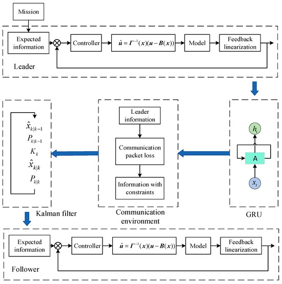
Figure 4. Formation predictive control framework.

4.2.2. GRU Neural Network

A GRU neural network is an improved recurrent neural network (RNN). A GRU is used to predict the future state of the leader UUV in this design. It is a variant of an RNN with a simpler structure and higher computational efficiency, and it also effectively mitigates the problem of gradient vanishing in the RNN. The internal structure of the GRU network is shown in Figure 5.

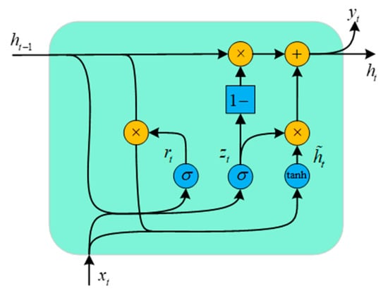
Figure 5. Internal structure of GRU network.

The process of the GRU network is as follows:

(1) The reset gate $r_t$ receives the state information $h_{t-1}$ output by the network from the leader UUV at a time of $t-1$ and the state information $x_t$ input by the network at a time of $t$, and calculates the degree of forgetfulness of the network for the information at a time of $t-1$; the calculation formula is

$$r_t=\sigma \left(W_r\cdot \left[h_{t-1},x_t\right]\right)$$

(32)

where $\sigma$ is the Sigmoid function, which is the activation function of the network, and $W_r$ is the weight matrix of the reset gate $r_t$.

(2) The update gate $z_t$ receives the same state information as the reset gate $r_t$ and calculates the degree of information inflow from moment $r_t$ to moment $t$; the formula is

$$z_t=\sigma \left(W_z\cdot \left[h_{t-1},x_t\right]\right)$$

(33)

where $W_z$ is the weight matrix of the update gate $z_t$.

(3) To obtain the $t$ moment activation state ${\tilde{h}}_t$, we combine the result of the reset gate $r_t$ acting on the $t-1$ moment $h_{t-1}$ with that of the $t$ moment network input $x_t$, and then introduce these results into the weight matrix $W_h$ multiplication, and obtain the final result using the tanh activation function. The formula for calculating the momentary activation state ${\tilde{h}}_t$ is as follows:

$${\tilde{h}}_t=\tanh \left(W_h\cdot \left[r_t\otimes h_{t-1},x_t\right]\right)$$

(34)

where $W_h$ is the weight matrix of the activation state ${\tilde{h}}_t$.

(4) We add the information retained by the network at moment $t-1$ with the activation state after the selection of the update gate $z_t$ at moment $t$; then, the output of the network at moment $t$ can be obtained, and is denoted as $h_t$ $t$. The output of moment $h_t$ is calculated using the formula

$$h_t=\left(1-z_t\right)\otimes h_{t-1}+{\tilde{h}}_t\otimes z_t$$

(35)

(5) The predicted state of the next moment of the output layer of the GRU network is calculated using the formula

$$y=\sigma \left(W_y\cdot h_t\right)$$

(36)

where $W_y$ is the weight matrix of the output layer, and $y$ is the output of the GRU network.

4.2.3. Kalman Filter

A Kalman filter (KF) is a recursive algorithm for estimating the state of a dynamic system and is used in this design to fuse the predicted and observed system state data to achieve optimal estimation of the system state; the flow of this algorithm is shown in Figure 6.

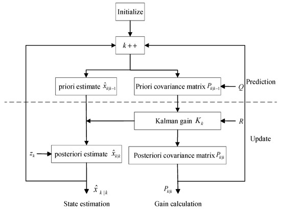
Figure 6. Kalman filtering algorithm.

Assume that the state space equation of the leader UUV is

$$x_k=A{x}_{k-1}+B{u}_{k-1}+w_{k-1}$$

(37)

where $x_k$ is the state vector at moment $k$; $A$ is the system state transfer matrix; $B$ is the system input matrix; $u_{k-1}$ is the system control input vector; and $w_{k-1}$ is the process noise.

Suppose the observation equation of the system is

$$z_k=H{x}_k+v_k$$

(38)

where $z_k$ is the observation vector at the time $k$; $H$ is the observation matrix; $v_k$ is the measurement noise, which is assumed to be zero-mean Gaussian white noise; and the covariance matrix is $R$.

$$v\sim N(0,R)$$

(39)

In the prediction stage, Kalman filtering utilizes the system model to make a priori estimate of the next moment ${\widehat{x}}_{k|k-1}$:

$${\widehat{x}}_{k|k-1}=A{\widehat{x}}_{k-1|k-1}+B{u}_{k-1}$$

(40)

where ${\widehat{x}}_{k|k-1}$ is the state prediction at moment $k$, also known as the a priori estimate, and ${\widehat{x}}_{k-1|k-1}$ is the state estimate at moment $k-1$.

The a priori estimate ${\widehat{x}}_{k|k-1}$ lacks the influence of the process noise $w_{k-1}$, unlike the state variable $x_k$, and it is also calculated by replacing the true value of the previous moment with the a posteriori estimate ${\widehat{x}}_{k-1|k-1}$ at the previous moment.

At the same time, Kalman filtering also uses the a posteriori error covariance matrix $P_{k-1|k-1}$ of the previous moment and the process noise covariance matrix array $Q$ to calculate the a priori error covariance matrix $P_{k|k-1}$.

$$P_{k|k-1}=A{P}_{k-1|k-1}{A}^T+Q$$

(41)

where $P_{k-1|k-1}$ is the a posteriori error covariance matrix at $k-1$, and $Q$ is the process noise covariance matrix.

We calculate the Kalman gain $K_k$ as follows:

$$K_k=P_{k|k-1}{H}^T{\left(H{P}_{k|k-1}{H}^T+R\right)}^{-1}$$

(42)

where $R$ is the covariance matrix of the measurement noise.

Next, we update the a posteriori estimate ${\widehat{x}}_{k|k}$ based on the a priori estimate ${\widehat{x}}_{k|k-1}$, the measured value $z_k$, and the Kalman gain $K_k$.

$${\widehat{x}}_{k|k}={\widehat{x}}_{k|k-1}+K_k\left(z_k-H{\widehat{x}}_{k|k-1}\right)$$

(43)

The a posteriori estimate ${\widehat{x}}_{k|k}$ is the optimal estimate output by the Kalman filtering algorithm after fusing the a priori estimate ${\widehat{x}}_{k|k-1}$ and the measurement value $z_k$.

4.2.4. Formation Prediction Model Based on GRU-KF

The GRU-KF-based formation prediction model is primarily composed of a GRU network prediction module and a Kalman filter module, as shown in Figure 7.

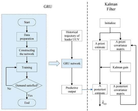
Figure 7. Formation prediction model based on GRU-KF.

The equation updating the state of the leader UUV can be expressed as

$$x_k=\left[\begin{array}{c}{\eta }_k\\ {\dot{\eta }}_k\end{array}\right]=\left[\begin{array}{cc}{I}_5& I_5\cdot t_0\\ O_5& I_5\end{array}\right]\cdot \left[\begin{array}{c}{\eta }_{k-1}\\ {\dot{\eta }}_{k-1}\end{array}\right]+w_{k-1}$$

(44)

where ${\eta }_k={\left[\begin{array}{lllll}{x}_k\hfill & y_k\hfill & z_k\hfill & {\theta }_k\hfill & {\psi }_k\hfill \end{array}\right]}^T$ represents the position and attitude of the leader UUV in the inertial coordinate system; ${\dot{\eta }}_k={\left[\begin{array}{lllll}{\dot{x}}_k\hfill & {\dot{y}}_k\hfill & {\dot{z}}_k\hfill & {\dot{\theta }}_k\hfill & {\dot{\psi }}_k\hfill \end{array}\right]}^T$ represents the velocity and angular velocity of the leader UUV in the inertial coordinate system; $I_5$ is the five-dimensional unit matrix; $O_5$ is the five-dimensional zero matrix; and $t_0$ is the control period of the leader UUV’s control system.

The transformation relationship between ${\dot{\eta }}_k$ and the velocity of the UUV in the carrier coordinate system is

$${\dot{\eta }}_k=\left[\begin{array}{l}{\dot{x}}_k\hfill \\ {\dot{y}}_k\hfill \\ {\dot{z}}_k\hfill \\ {\dot{\theta }}_k\hfill \\ {\dot{\psi }}_k\hfill \end{array}\right]=\left[\begin{array}{lllll}\cos \theta \cos \psi \hfill & -\sin \psi \hfill & \sin \theta \cos \psi \hfill & 0\hfill & 0\hfill \\ \cos \theta \sin \psi \hfill & \cos \psi \hfill & \sin \theta \sin \psi \hfill & 0\hfill & 0\hfill \\ -\sin \theta \hfill & 0\hfill & \cos \theta \hfill & 0\hfill & 0\hfill \\ 0\hfill & 0\hfill & 0\hfill & 1\hfill & 0\hfill \\ 0\hfill & 0\hfill & 0\hfill & 0\hfill & 1/\cos \theta \hfill \end{array}\right]\cdot \left[\begin{array}{l}u\hfill \\ v\hfill \\ w\hfill \\ q\hfill \\ r\hfill \end{array}\right]$$

(45)

The system model is established as follows:

$$z_k=\left[\begin{array}{c}{\eta }_k\\ {\eta }_k^v\end{array}\right]=\left[\begin{array}{cc}{I}_5& O_5\\ O_5& J(\eta {)}^{\prime }\end{array}\right]\cdot \left[\begin{array}{c}{\eta }_k\\ {\dot{\eta }}_k\end{array}\right]+v_k$$

(46)

where ${\eta }_k^v={\left[\begin{array}{lllll}u\hfill & v\hfill & w\hfill & q\hfill & r\hfill \end{array}\right]}^T$ is the velocity of the leader UUV in the carrier coordinate system, and $J(\eta )$ is the transformation matrix from the carrier coordinate system to the inertial coordinate system of the leader UUV.

5. Simulation

To verify the effectiveness of the GRU-KF-based UUV formation-control strategy proposed in this paper, we conduct simulation verification of UUV formation control based on the leader–follower method and in a communication packet loss environment.

5.1. Simulation and Analysis of UUV Formation Control Based on Leader–Follower Method

This section focuses on the simulation verification of the UUV formation controller based on the leader–follower method and analyzes the formation-control effect. In the simulation experiment, the desired trajectory of the leader UUV₁ is

$$\left\{\begin{array}{ll}{x}_d=250\cos (2\pi t/1000)\hfill & \hfill \\ y_d=250\sin (2\pi t/1000)\hfill & 0\le t\le 1500\hfill \\ z_d=-0.015t-5\hfill & \hfill \end{array}\right.$$

(47)

Initial state of UUVs:

Leader UUV₁: northward coordinate $x_1=249.5 \mathrm{m}$, eastward coordinate $y_1=1 \mathrm{m}$, vertical coordinate $z_1=-3 \mathrm{m}$, yaw angle ${\psi }_1=\pi /2 \mathrm{rad}$, longitudinal velocity $u_1=1 \mathrm{m}/\mathrm{s}$, and remaining initial states have value of 0.

Follower UUV₂: northward coordinate $x_2=205.5 \mathrm{m}$, eastward coordinate $y_2=-49 \mathrm{m}$, vertical coordinate $z_2=-3.5 \mathrm{m}$, yaw angle ${\psi }_2=\pi /2 \mathrm{rad}$, longitudinal velocity $u_2=1 \mathrm{m}/\mathrm{s}$, and remaining initial states have value of 0.

Follower UUV₃: northward coordinate $x_3=298.5 \mathrm{m}$, eastward coordinate $y_3=-50.1 \mathrm{m}$, vertical coordinate $z_3=-4.5 \mathrm{m}$, yaw angle ${\psi }_3=\pi /2 \mathrm{rad}$, longitudinal velocity $u_3=1 \mathrm{m}/\mathrm{s}$, and remaining initial states have value of 0.

Formation parameters: $L=50\sqrt{2}$ and $\beta =\pi /4$.

The uncertainty term of the UUV model is

$$\left\{\begin{array}{ll}{\Delta }_1=0.5(\sin (0.3t\times 0.1)+\cos (0.5t\times 0.1))\hfill & \hfill \\ {\Delta }_2=0.5(\sin (0.3t\times 0.1)+\cos (0.05t\times 0.1))\hfill & \hfill \\ {\Delta }_3=0.5(\sin (0.02t\times 0.1)+\cos (0.4t\times 0.1))\hfill & 0\le t\le 1500\hfill \\ {\Delta }_4=0.2(\sin (0.03t\times 0.1)+\cos (0.04t\times 0.1))\hfill & \hfill \\ {\Delta }_5=0.2(\sin (0.03t\times 0.1)+\cos (0.4t\times 0.1))\hfill & \hfill \end{array}\right.$$

(48)

The parameters of the backstepping sliding mode controller based on the RBF neural network are $c_1=1.5$, $k_1=1.2$, and $\eta =0.3$. The initial weights of the RBF network are all 0.02, and the adaptive parameters are $c_i=\left[\begin{array}{lllllllllll}-10\hfill & -3\hfill & -1\hfill & -0.5\hfill & -0.1\hfill & 0\hfill & 0.1\hfill & 0.5\hfill & 1\hfill & 3\hfill & 10\hfill \end{array}\right]$, $\gamma =50$, and $b_j=6$. The parameter $K=0.8$, the current interference is $v_{current1}^E=\left[\begin{array}{ccc}0.2& 0& 0\end{array}\right] \mathrm{m}/\mathrm{s}$, and the simulation time is 1500 s.

Figure 8a–e show the position and attitude errors of the UUV formation. At 46 s, the formation gradually stabilizes. The maximum absolute errors for all three axes are less than 0.1 m, the longitudinal tilt steady-state error is less than 0.001 rad, and the maximum absolute error for the heading angle is less than 0.03 rad. Even under the influence of the current disturbance and model uncertainty constraints, the preset UUV formation can still be formed and maintained, and both the position and the attitude errors are limited and kept within a small range. Figure 8f–j show the velocity and angular velocity errors of the UUV formation. At 36 s, the angular velocity error converges, and the maximum absolute error of the three-axis speed is less than 0.05 m/s. The velocity and angular velocity of the UUV formation are still able to track the upper desired value, even under the influence of the current interference and model uncertainty constraints, and the errors are all limited and kept within a small range, which validates the effectiveness of the formation-control strategy.

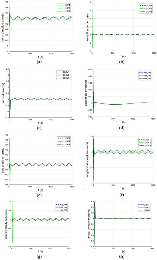
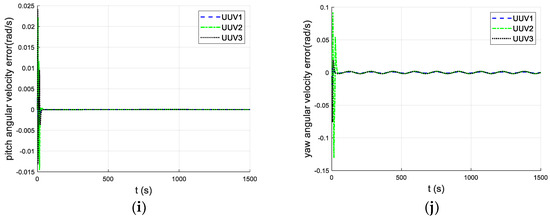
Figure 8. (a) North direction error; (b) east direction error; (c) vertical error; (d) pitch angle error; (e) yaw angle error; (f) longitudinal speed error; (g) lateral velocity error; (h) vertical velocity error; (i) pitch angular velocity error; (j) yaw angular velocity error.

Figure 9 shows a two-dimensional trajectory diagram of the UUV formation, and Figure 10 shows a three-dimensional trajectory diagram of the UUV formation. Even under the influence of current interference and model uncertainty, the preset UUV formation is able to be maintained, and the spiral dive motion in 3D space can be completed, further verifying the effectiveness of the formation-control strategy presented in this section.

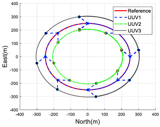
Figure 9. Two-dimensional trajectory of UUV formation.

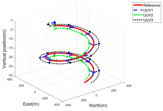
Figure 10. Three-dimensional trajectory of UUV formation.

5.2. Simulation and Analysis with Communication Packet Loss

To analyze the effect of communication packet loss on UUV formation control, we consider simulation verification with a 10% packet loss rate and set the leader to broadcast its own state information every 4 s. The other condition settings of the simulation are kept consistent with those described in Section 5.1. The key parameters for the GRU network training process are as follows: the maximum number of training rounds is set to 5, and the gradient clipping threshold is set to 1. To optimize the learning rate adjustment strategy, the initial learning rate is set to 0.001, and a piecewise learning rate decay mode is adopted, where the learning rate is reduced by 90% every two training rounds; i.e., the decay factor is 0.1. Additionally, to improve computational efficiency, mini-batch training is employed during the training process, with the batch size set to 16. The simulation results are as follows:

Figure 11a–e compare the follower’s position and attitude errors after the prediction compensation based on the GRU-KF network prediction model with a 10% packet loss rate. It can be seen that when relying solely on the GRU network for compensation, because of communication packet loss, more obvious jitter occurred in several of the follower’s state variables at the time step where communication packet loss occurred, and the maximum error reached 13.8 m. This kind of obvious jitter is not allowed in application scenarios that require high control accuracy, as it may have a large impact on the control accuracy of the system. However, with GRU-KF algorithm compensation, the formation stabilized after 28 s, with the maximum absolute error of the three axes reaching less than 0.4 m. The pitch angle and heading angle error converged after 42 s, with the maximum angle error not exceeding 0.02 rad.

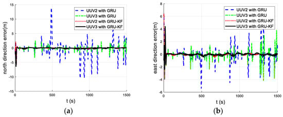
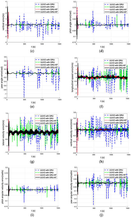
Figure 11. (a) North direction error; (b) east direction error; (c) vertical error; (d) pitch angle error; (e) yaw angle error; (f) longitudinal speed error; (g) lateral velocity error; (h) vertical velocity error; (i) pitch angular velocity error; (j) yaw angular velocity error.

Figure 11f–j compare the follower’s velocity and angular velocity errors after prediction compensation based on the GRU-KF network prediction model with a 10% packet loss rate. Similarly to the follower’s position error and attitude error, there is sudden jitter in the error curve at the time step where communication packet loss occurs when only the GRU network is used for compensation. When the GRU-KF network prediction model is used for compensation, the absolute values of the maximum errors in both longitudinal and transverse velocities are both less than 0.3 m/s. The error in vertical velocity converges at 37 s, with the maximum error not exceeding 0.01 m/s. The error in angular velocity converges at 39 s, with the maximum errors all being less than 0.01 rad/s.

It can be concluded that with the constraint of a 10% packet loss rate, the GRU-KF network prediction model can effectively compensate for the problem of data loss caused by communication packet loss, and the error curves of the follower’s position, attitude, velocity, and angular velocity are smoother. In addition, error fluctuation is significantly reduced, preventing the generation of sudden errors and improving the stability of formation control.

6. Conclusions

In this study, the problem of formation control in UUVs with the constraint of packet loss is investigated, and a predictive control method based on the GRU-KF network prediction model is proposed to improve the control accuracy and stability of the system in complex environments. To address these problems, a GRU-KF-based formation predictive control strategy is constructed, where the GRU network is used for short-term prediction of the leader trajectory, while the KF is used to combine the GRU prediction results with the a priori estimation of the system state equations to compensate for the uncertainty caused by communication packet loss and positioning errors. Finally, the effectiveness of the GRU-KF network prediction model is verified through simulation experiments. With communication packet loss, the GRU-KF network prediction model can effectively prevent the generation of sudden errors.

In practical applications, the problem of collisions between UUVs cannot be ignored. A collision avoidance algorithm is not proposed in this study; however, future research should endeavor to develop an effective solution to this problem.

References

- Li, H.; Cui, S.; Wang, X.; Yu, B.; Wang, G.; Cao, C.; Shen, Y.; Zeng, Q. Development of a bionic jellyfish robot for collecting polymetallic nodules. Ocean. Eng. 2025, 324, 120655. [Google Scholar] [CrossRef]
- Subin Raj, V.B.; Sarun Lal, M.A.; Gowri, R.S.; Ramesh, S.; Ramesh, N.R.; Ramesh, R.; Deepak, V.; Vadivelan, A.; Ramadass, G.A. Assessment of polymetallic nodules in the Central Indian Ocean Basin: Factors influencing distribution patterns through high-resolution autonomous underwater vehicle (AUV) survey. Geo-Mar. Lett. 2025, 45, 7. [Google Scholar] [CrossRef]
- Zhu, H.; Chen, J.; Lin, Y.; Zhou, P.; Wang, K.; Lin, P.; Peng, X.; Li, H.; Guo, J.; Ren, X.; et al. The application of structured light for external subsea pipeline inspection based on the underwater dry cabin. Appl. Ocean. Res. 2025, 155, 104431. [Google Scholar] [CrossRef]
- Sang, I.-C.; Norris, W.R. An Adaptive Image Thresholding Algorithm Using Fuzzy Logic for Autonomous Underwater Vehicle Navigation. IEEE J. Sel. Top. Signal Process. 2024, 18, 358–367. [Google Scholar] [CrossRef]
- Patel, S.; Abdellatif, F.; Alsheikh, M.; Trigui, H.; Outa, A.; Amer, A.; Sarraj, M.; Al Brahim, A.; Alnumay, Y.; Felemban, A.; et al. Multi-robot system for inspection of underwater pipelines in shallow waters. Int. J. Intell. Robot. Appl. 2024, 8, 14–38. [Google Scholar] [CrossRef]
- Feng, W.; Ma, Y.; Li, H.; Liu, H.; Meng, X.; Zhou, M. Optimal search path planning of UUV in battlefeld ambush scene. Def. Technol. 2024, 32, 541–552. [Google Scholar] [CrossRef]
- sub Song, K.; Chu, P.C. Conceptual design of future undersea unmanned vehicle (UUV) system for mine disposal. IEEE Syst. J. 2012, 8, 43–51. [Google Scholar] [CrossRef]
- Yan, Z.; Yan, J.; Cai, S.; Yu, Y.; Wang, Y.; Hou, S. Distributed TMPC formation trajectory tracking of multiple underwater unmanned vehicles with uncertainties and external perturbations. Ocean Eng. 2024, 298, 117160. [Google Scholar] [CrossRef]
- Yan, Z.; Yang, Z.; Pan, X.; Zhou, J.; Wu, D. Virtual leader based path tracking control for multi-UUV considering sampled-data delays and packet losses. Ocean Eng. 2020, 216, 108065. [Google Scholar] [CrossRef]
- Chen, Y.; Guo, X.; Luo, G.; Liu, G. A Formation Control Method for AUV Group Under Communication Delay. Front. Bioeng. Biotechnol. 2022, 10, 848641. [Google Scholar] [CrossRef] [PubMed]
- Li, J.; Tian, Z.; Zhang, H. Discrete-time AUV formation control with leader-following consensus under time-varying delays. Ocean Eng. 2023, 286, 115678. [Google Scholar] [CrossRef]
- Jiang, X.; Xia, G. Nonfragile formation control of leaderless unmanned surface vehicles with memory sampling data and packet loss. IEEE Syst. J. 2022, 17, 3026–3035. [Google Scholar] [CrossRef]
- Kuniyoshi, S.; Oshiro, S.; Saotome, R.; Wada, T. An Iterative Orthogonal Frequency Division Multiplexing Receiver with Sequential Inter-Carrier Interference Canceling Modified Delay and Doppler Profiler for an Underwater Multipath Channel. Mar. Sci. Eng. 2024, 12, 1712. [Google Scholar] [CrossRef]
- Yan, Z.P.; Pan, X.L.; Yang, Z.W.; Yue, L.D. Formation Control of Leader-Following Multi-UUVs With Uncertain Factors and Time-Varying Delays. IEEE Access 2019, 7, 118792–118805. [Google Scholar] [CrossRef]
- Saleem, K.; Wang, L.; Bharany, S. Survey of AI-driven routing protocols in underwater acoustic networks for enhanced communication efficiency. Ocean Eng. 2024, 314, 119606. [Google Scholar] [CrossRef]
- Yan, Z.; Yan, J. Self-triggered formation control of asynchronous multiple underwater unmanned vehicle under communication delay. Unmanned Syst. 2024. [Google Scholar] [CrossRef]
- Cai, W.; Ju, Y.; Liu, Z.; Zhang, M.; Lv, S. Event-triggered leader-follower communication based formation control with dual-predictor for multiple AUVs. Ocean Eng. 2025, 334, 121552. [Google Scholar] [CrossRef]
- Tang, C.; Shi, H.; Zhang, L. Trajectory planning aided unmanned surface vehicle optimization communication method with hierarchical reinforcement learning. Ocean Eng. 2024, 307, 118225. [Google Scholar] [CrossRef]
- Liu, Y. Research on Coordinated Control Methods for Ocean Surveying by Underwater Vehicle Fleets. Ph.D. Dissertation, Harbin Engineering University, Harbin, China, 2017. [Google Scholar]
- Nettari, Y.; Kurt, S.; Labbadi, M. Adaptive Robust Control based on Backstepping Sliding Mode techniques for Quadrotor UAV under external disturbances. IFAC-PapersOnLine 2022, 55, 252–257. [Google Scholar] [CrossRef]
- Du, P.; Yang, W.; Wang, Y.; Hu, R.; Chen, Y.; Huang, S. A novel adaptive backstepping sliding mode control for a lightweight autonomous underwater vehicle with input saturation. Ocean Eng. 2022, 263, 112362. [Google Scholar] [CrossRef]
- Yan, Z.; Jiang, A.; Lai, C.; Li, H. Velocity-Free Formation Control and Collision Avoidance for UUVs via RBF: A High-Gain Approach. Electronics 2022, 11, 1170. [Google Scholar] [CrossRef]
- Wang, H.; Ren, J.; Han, M.; Wang, Z.; Zhang, K.; Wang, X. Robust adaptive three-dimensional trajectory tracking control for unmanned underwater vehicles with disturbances and uncertain dynamics. Ocean Eng. 2023, 289, 116184. [Google Scholar] [CrossRef]
- Huang, C.; Xu, H.; Batista, P.; Zhang, X.; Soares, C.G. Fixed-time leader-follower formation control of underactuated unmanned surface vehicles with unknown dynamics and ocean disturbances. Eur. J. Control 2023, 70, 100784. [Google Scholar] [CrossRef]
Disclaimer/Publisher’s Note: The statements, opinions and data contained in all publications are solely those of the individual author(s) and contributor(s) and not of MDPI and/or the editor(s). MDPI and/or the editor(s) disclaim responsibility for any injury to people or property resulting from any ideas, methods, instructions or products referred to in the content. |
© 2025 by the authors. Licensee MDPI, Basel, Switzerland. This article is an open access article distributed under the terms and conditions of the Creative Commons Attribution (CC BY) license (https://creativecommons.org/licenses/by/4.0/).