FLUID: Dynamic Model-Agnostic Federated Learning with Pruning and Knowledge Distillation for Maritime Predictive Maintenance

Abstract

Predictive maintenance (PdM) is vital to maritime operations; however, the traditional deep learning solutions currently offered heavily depend on centralized data aggregation, which is impractical under the limited connectivity, privacy concerns, and resource constraints found in maritime vessels. Federated Learning addresses privacy by training models locally, yet most FL methods assume homogeneous client architectures and exchange full model weights, leading to heavy communication overhead and sensitivity to system heterogeneity. To overcome these challenges, we introduce FLUID, a dynamic, model-agnostic FL framework that combines client clustering, structured pruning, and student–teacher knowledge distillation. FLUID first groups vessels into resource tiers and calibrates pruning strategies on the most capable client to determine optimal sparsity levels. In subsequent FL rounds, clients exchange logits over a small reference set, decoupling global aggregation from specific model architectures. We evaluate FLUID on a real-world heavy-fuel-oil purifier dataset under realistic heterogeneous deployment. With mixed pruning across clients, FLUID achieves a global $R^2$ of 0.9352, compared with 0.9757 for a centralized baseline. Predictive consistency also remains high for client-based data, with a mean per-client MAE of 0.02575 ± 0.0021 and a mean RMSE of 0.0419 ± 0.0036. These results demonstrate FLUID’s ability to deliver accurate, efficient, and privacy-preserving PdM in heterogeneous maritime fleets.

1. Introduction

Predictive maintenance (PdM) plays a crucial role in maritime operations, where minimizing unplanned downtime and optimizing machinery health impacts safety, operational efficiency, and costs [1]. Recent advancements in deep learning (DL) have empowered data-driven PdM models to forecast component degradation, detecting anomalies, and estimating a component’s remaining useful life (RUL) [2,3,4]. However, these models typically rely on Centralized Machine Learning (CML) architectures, where raw sensor data coming from the vessels are transmitted to a central server for model training. While this is effective, such approaches can face major obstacles in real-world maritime environments due to limited connectivity, privacy requirements, and high communication costs [5,6].

Federated Learning (FL) offers a promising alternative by enabling model training directly on device, allowing clients to collaboratively learn from distributed data without exposing them. This approach is particularly attractive in maritime applications, where edge computing is increasingly used to manage data locally [7]. Despite its benefits, FL is not without limitations, especially concerning the aspect of potential heterogeneous and resource-constrained maritime fleets [8,9].

One of the most critical challenges in FL is system heterogeneity, where clients may differ significantly in memory, computation capacity, energy constraints, bandwidth availability, etc. These disparities can lead to the straggler effect, where slower devices delay global model updates, impacting convergence or causing complete training failure if too many clients cannot keep up. While some works exclude these underperforming clients, this action can potentially introduce bias to the global model, by ignoring clients that may hold valuable or representative data [9,10]. Furthermore, another challenge is statistical heterogeneity, where the distribution of data varies widely across clients. Many FL strategies, such as FedAvg [11] or FedProx [12], attempt to address this by averaging weights or modifying local objectives. Still, they assume uniform model architectures and identical computational resources across all participants, an often unrealistic constraint in diverse and dynamic environments like those found in the maritime domain [13,14].

Furthermore, most existing PdM models used in CML or FL frameworks are computationally heavy, requiring large memory footprints and prolonged inference times, making them impractical for deployment on constrained onboard hardware [15,16]. This highlights the need for lightweight, adaptable FL frameworks that preserve performance while accommodating the diverse client capabilities and models.

To address these challenges, we propose FLUID, a novel, communication-efficient FL framework that supports heterogeneity in both models and system resources (i.e., model and system agnostic). FLUID replaces weight sharing with a student–teacher knowledge distillation mechanism, allowing clients to learn from compact logit representations instead of full model parameters [17,18]. This decouples the global model structure from client architectures, enabling each vessel to use models tailored to its local constraints without sacrificing global performance [19,20,21].

Toward this direction, the main contributions of this work include the following:

• We introduce FLUID, a lightweight, model architecture-agnostic FL framework that enables collaboration among heterogeneous clients in maritime environments;
• We develop a logit-based knowledge exchange mechanism that eliminates the need for full model synchronization while preserving predictive performance to achieve faster convergence and high robustness;
• We design a dynamic clustering module that groups client ships into resource tiers, enabling the calibration of structured pruning strategies, guaranteeing model compression and respecting the heterogeneous computing constraints without manual tuning;
• We conduct a comprehensive evaluation using real-world maritime PdM data, demonstrating that FLUID achieves competitive accuracy against state-of-the-art CML and FL strategies that do not incorporate heterogeneous model architectures.

The remainder of this paper is organized as follows: Section 2 provides background on HFO purification systems and reviews state-of-the-art PdM approaches for maritime applications, along with the relevant FL literature addressing model heterogeneity. Section 3 describes the experimental setup, including the dataset, feature preprocessing, model architectures, pruning strategies, and evaluation metrics. Section 4 presents the results of this study, while Section 5 concludes with a summary of findings, limitations, and directions for future work.

2. Background and Related Work

2.1. Heavy-Fuel-Oil Purifier

For over six decades, HFO has been the primary fuel choice in the maritime industry, due to its cost-effectiveness and widespread availability. However, HFO contains significant quantities of catalytic fines and other impurities, which must be consistently maintained at low levels to safeguard the engine’s operational efficiency [22,23,24]. For this task, vessels are equipped with HFO purifiers, facilitating the delivery of clean fuel to the ME and auxiliary systems by separating impurities (i.e., water and solid particles) from the fuel, thus preventing ineffective combustion and damage to critical equipment (e.g., fuel pumps, injectors, and nozzles).

In practice, the efficiency of purifiers tends to decline over time, increasing the risk of contaminants reaching engine equipment. Currently, to mitigate this, overhaul operations are carried out by specialized personnel either when abnormal sings are detected (increased vibration, worn gear components, etc.) or according to the PM schedules [25]. Nevertheless, because purifiers operate at high rotation speeds and consist of intricate components, they remain vulnerable to failures if not properly or timely maintained [26].

2.2. PdM in the Maritime Domain

Recent works have explored DL-based PdM solutions for maritime applications, targeting key performance metrics such as the estimation of the RUL of critical vessel components [27,28,29]. For instance, in [30], a hybrid model of a Convolutional Neural Networks (CNNs) and a bi-directional gated recurrent units was introduced to predict the Exhaust Gas Temperature (EGT). Model efficiency has also been explored in the PdM literature. For example, in [23], CNN and AutoEncoder (AE) models were combined with early stopping and pruning to predict the RUL of HFO purification systems, aiming to deploy PdM solutions under onboard resource constraints vessels. In [31], the authors introduced the DELTA framework, applying degradation-aware Hilbert–Huang transformation with an LSTM-AE model to estimate the RUL of engine bearings.

FL has also gained popularity in maritime PdM applications, offering privacy-preserving collaboration across vessels. For example, initial studies include the work in [32], which investigated the prediction of decay of a gas turbine by evaluating different FL strategies (i.e., FedAvg, FedSGD, FedProx, and FedAvgM) with a fully connected NN model. Furthermore, FedShip leverages the computation of Over-the-Air aggregation in next-generation maritime networks, targeting ME propulsion power prediction. The framework was benchmarked against CML, transfer learning, and ensemble methods, achieving high MAE scores, close to CML, while reducing communication overhead in dense client scenarios [33].

These efforts highlight that most maritime PdM models to date are trained via centralized learning (CML), and FL, while emerging, remains underexplored in maritime PdM contexts. Furthermore, many CML-based models are considered computationally intensive, requiring significant memory and processing resources during training and inference, posing challenges for real-world deployment on edge-constrained maritime platforms, where bandwidth, compute capacity, and power availability can be limited. As a result, there is a growing need for lightweight, secure, and modular learning frameworks that enable local training on heterogeneous hardware and model architectures without sacrificing predictive performance [34,35,36].

2.3. Federated Learning

FL was first introduced by Google in 2016 to train shared models directly on users’ devices, transmitting only weight updates rather than raw data [11,36]. This client--server paradigm dramatically reduces privacy risks and bandwidth requirements in contrast to traditional CML training by keeping sensitive information local [37,38]. The seminal FedAvg algorithm [11] simply averages client updates at each round, but it struggles when client data distributions or system capabilities vary widely. To address statistical heterogeneity, strategies like FedProx add a proximal term to clients’ objectives [12], while FedNova re-normalizes local updates to avoid bias [39], and SCAFFOLD employs control variates to correct for “client drift” [40]. Although these extensions can improve convergence, they are subject to several critical limitations, as they still exchange full model weights at each round, incurring heavy communication and entangling accuracy with each client’s architecture [41].

2.4. Model Pruning for Communication Efficiency

Model pruning techniques, i.e., removing the redundant model weights or filters, have been widely applied to compress networks [42,43]. In the FL setting, pruning can reduce the size of each client’s transmitted updates [44,45], but naïve approaches may degrade accuracy or require expensive re-training on resource-limited devices [46]. Recent work explores adaptive, structured pruning that dynamically adjusts to device constraints yet still assumes a shared global architecture, limiting flexibility towards clients running on either heterogeneous resources or models. For instance, [47] introduced AdaptCL, a dynamic multi-party collaborative pruning method enabling sparsity decisions to be made according to the client model’s performance, substantially reducing data transitions during training rounds and adding, however, additional computational complexity. Similarly, [48] proposed AutoFLIP, an FL adaptive pruning method that incorporates a federated loss exploration phase to minimize computational overhead, not assuming hierarchical environments with diverse client resources or different model structures.

2.5. Knowledge Distillation and Ensembles in FL

Knowledge distillation (KD) transfers knowledge from a large “teacher” to a smaller “student” network [17,49], and ensembles of teachers can further boost performance [18,50,51]. In FL, KD has been leveraged to both address heterogeneity and cut communication. For example, FedDF distills an ensemble of client teachers into a global student at the server [52], and FedKD performs mutual distillation between student and teacher locally [19]. These approaches trade weight exchange for smaller “knowledge payloads,” but require joint public datasets or demand that all clients share the same model backbone. Recent works target fundamentally heterogeneous clients. Another approach includes AvgKD, which lets a client receive all available models coming from the of the participating clients, computing an average logit based on all the logits received from the peers. This approach has been shown to scale poorly when many clients participate in the process, significantly increasing the computational overhead [53]. GeFL uses generative models to align representations but depends on auxiliary generators [54], and FedAKD applies student–teacher KD across networks under non-IID splits, achieving impressive communication savings but not accounting for the client resource capabilities to run these models [20].

Unlike existing FL approaches that depend on full model weight exchange or assume a shared model architecture, FLUID introduces a tailored framework for the heterogeneous and resource-constrained maritime domain. By adopting a student–teacher knowledge distillation paradigm, FLUID enables clients to train model variants best suited to their local capabilities, without requiring architectural uniformity, while still achieving satisfactory accuracy compared with traditional weight-based aggregation methods.

3. FLUID Framework Overview

In this section, we present the FLUID framework, including its underlying model and assumptions, and describe in detail how FLUID optimizes client collaboration for training PdM models.

3.1. System Model and Basic Assumptions

For the description of the FLUID framework, we consider a maritime PdM scenario including a fleet of bulk carrier ships, each equipped with on-board sensors collecting time-series data for machinery monitoring. Our system follows a classical server–client architecture. Specifically, the server is hosted on an onshore control center (e.g., maritime company headquarters) with computation and storage facilities. This server is responsible for coordinating the federated rounds, aggregating model updates and dispatching global parameters. Clients, on the other hand, include ships $i\in \mathcal{C}=1,\dots ,N$ running local training and inference. Each client holds a private dataset $D_i$ of labeled sensor readings and derives a resource profile ${\mathbf{r}}_i={[{\mathrm{CPU}}_i,{\mathrm{GPU}}_i,{\mathrm{RAM}}_i]}^{\top }$. Furthermore, to realize this scenario, the following assumptions are followed:

1.

Data heterogeneity: Local datasets $D_i$ exhibit non-IID label distribution due to differing ship usage patterns.

2.

Resource heterogeneity: Ships vary widely in compute and memory capacities; we assume that $|{\mathbf{r}}_i{|}_2$ accurately reflects available resources.

3.

Communication constraints: Clients communicate with the server over high-latency satellite links; the number of communication rounds R is, therefore, limited.

4.

Security and privacy: Raw sensor data remain on device; only model parameters or logits are exchanged. However, the practical implementation of knowledge distillation relies on a small, unlabeled public reference dataset $D_p$. In the context of a single maritime company, this dataset does not need to be externally sourced, as it can be constructed from a small fraction of historical, anonymized sensor readings stored in a central server that is a trusted entity within the organization.

3.2. Dynamic Pruning Adaptation to Client Resources

Before pruning calibration, clients are grouped into K resource tiers via a clustering function based on their normalized profiles ${\left\{{\mathbf{r}}_i\right\}}_{i=1}^N$. This unsupervised step allows FLUID to adaptively calibrate model compression levels in accordance with the actual compute and memory capabilities of the fleet.

$$\left\{{\mathcal{C}}_1,{\mathcal{C}}_2,\dots ,{\mathcal{C}}_K\right\}=\mathrm{Cluster}\left({\left\{{\mathbf{r}}_i\right\}}_{i=1}^N,K\right)$$

(1)

where cluster denotes any suitable clustering method applied to normalized resource profiles, K is selected based on domain knowledge or clustering criteria, and ${\mathcal{C}}_1$ denotes the highest resource tier. From this group, client $i^{*}$ with maximum resource norm is selected as primary candidate for pruning calibration following [44]:

$$i^{*}=arg\underset{i\in {\mathcal{C}}_1}{max}{\parallel {\mathbf{r}}_i\parallel }_2.$$

(2)

Clients periodically report their resource profile. If $i^{*}$ becomes unavailable (e.g., due to networking or scheduling constraints), fallback selection proceeds to the next best client $\left(i^{**}\right)$ as in Equation (2). Similarly, clients that experience resource degradation may be reassigned to lower tiers and receive simpler models. As illustrated in Figure 1, the FLUID framework begins by dispatching the baseline model to the highest-resource client for pruning and tuning.

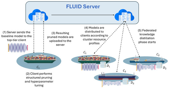
Figure 1. Overview of FLUID’s server-side model preparation and dispatch process.

In this calibration phase, we evaluate different pruning strategies, each implemented as a structured pruning operator ${\mathcal{P}}_t({\theta }^0,h)$ applied to the baseline model ${\theta }^0$, where t indexes the pruning method and h its hyperparameters (e.g., target sparsity). For each $t\in \mathcal{T}$ and $h\in {\mathcal{H}}_t$, we (i) apply pruning: ${\theta }^{(t,h)}={\mathcal{P}}_t({\theta }^0,h)$; (ii) train on $D_{i^{*}}$ for $E_0$ epochs, yielding ${\theta }_{i^{*}}^{(t,h)}$; and (iii) evaluate $D_{\mathrm{val}}$ and record $R^2$ performance.

$${R_{i^{*}}^2}^{(t,h)}=1-{\displaystyle \frac{{\sum }_j{(y_j-{\widehat{y}}_j)}^2}{{\sum }_j{(y_j-\overline{y})}^2}}$$

(3)

The pruning strategy $t^{*}$ with the highest validation $R^2$ is selected:

$$t^{*}=arg\underset{t\in \mathcal{T}}{max}\underset{h\in {\mathcal{H}}_t}{max}{R_{i^{*}}^2}^{(t,h)}$$

(4)

After finding the best pruning method $t^{*}$, we choose M sparsity levels from the search space $h\in {\mathcal{H}}_{t^{*}}$ to deploy across client tiers:

$$\{h^{\left(1\right)},h^{\left(2\right)},\dots ,h^{\left(M\right)}\}\subseteq H_t^{*}$$

(5)

Then, for $t^{*}$, we further refine the sparsity level by searching over $h\in {\mathcal{H}}_{t^{*}}$ to find

$${\left\{h\left(k\right)\right\}}_{k=1}^M=arg\underset{S\subseteq H,\left|S\right|=M}{max}\sum _{h\in S}{R}_{i^{*}}^2(t^{*},h)$$

(6)

Then we rank all $h\in {\mathcal{H}}_t*$ by their $R^2$ score on the validation set and pick the top M values. For example, when $M=2$ (i.e., three tiers), this reduces to selecting the two highest-scoring sparsities. The full model, moderately pruned model, and highly pruned model are then dispatched as follows:

$${\theta }_i\left(0\right)=\left\{\begin{array}{cc}{\theta }_0,\hfill & i\in C_1\hfill \\ P_t^{*}({\theta }^0,h^{\left(1\right)}),\hfill & i\in C_2\hfill \\ P_t^{*}({\theta }^0,h^{\left(2\right)}),\hfill & i\in C_3\hfill \\ ⋮\hfill & \\ P_t^{*}({\theta }^0,h^{(K-1)}),\hfill & i\in C_K\hfill \end{array}\right.$$

(7)

Algorithm 1 FLUID: server-side calibration and model dispatch.

1: Input: Number of tiers K, baseline model ${\theta }_0$, set of pruning methods $\mathcal{T}$   2: Initialize empty list of client profiles: $R_{\mathrm{profiles}}\leftarrow \left[\right]$   3: Initialize teacher: $Z_{\mathrm{current}}\left(x\right)\leftarrow \mathrm{InitialPredictions}(D_p,{\theta }_0)$   4: Phase 1a: Dynamic Pruning Adaptation   5: for each client $i\in \{1,\dots ,N\}$ do   6:     Client i reports its resource profile $r_i$   7:     Add $r_i$ to $R_{\mathrm{profiles}}$   8: end for   9: Group clients into K tiers: $\{{\mathcal{C}}_1,\dots ,{\mathcal{C}}_K\}\leftarrow \mathrm{Cluster}(R_{\mathrm{profiles}},K)$, where ${\mathcal{C}}_1$ is the highest-resource tier. 10: Select calibration client: $i^{*}\leftarrow arg{max}_{i\in {\mathcal{C}}_1}{\parallel r_i\parallel }_2$ 11: Find best pruning method $t^{*}$ by evaluating all $(t,h)$ on client $i^{*}$ 12: Select top $K-1$ sparsity levels $\{h^{\left(1\right)},\dots ,h^{(K-1)}\}$ for method $t^{*}$ based on $R^2$ performance on validation set 13: Phase 1b: Model Dispatch 14: for each tier $k\in \{1,\dots ,K\}$ do 15:     if $k=1$ then 16:         ${\theta }_{\mathrm{dispatch}}\leftarrow {\theta }_0$                                        \ Full baseline model for Tier 1 17:     else 18:         $h_{\mathrm{prune}}\leftarrow h^{(k-1)}$                                        \ $(k-1)$-th best sparsity level 19:         ${\theta }_{\mathrm{dispatch}}\leftarrow {\mathcal{P}}_{t^{*}}({\theta }_0,t^{*},h_{\mathrm{prune}})$ 20:     end if 21:     for each client $i\in {\mathcal{C}}_k$ do 22:         Send ${\theta }_{\mathrm{dispatch}}$ to client i                \ Initializes client’s local model ${\theta }_{\mathrm{local}}$ 23:     end for 24: end for

3.3. Federated Knowledge Distillation

Traditional Federated Learning strategies such as FedAvg [11] assume model homogeneity and perform round-wise parameter averaging:

$${\theta }^{(t+1)}=\sum _{i\in \mathcal{S}}{\displaystyle \frac{n_i}{{\sum }_{j\in \mathcal{S}}{n}_j}}·{\theta }_i^{\left(t\right)}$$

(8)

where ${\theta }^{(t+1)}$ is the global model at round $t+1$, S is the set of selected clients, $n_i$ is the number of data points at client i, and ${\theta }_i^{(t+1)}$ is the updated model from client i.

However, FedAvg requires all clients to maintain identical model architectures and parameter shapes, which is infeasible in heterogeneous resource environments, where clients can exhibit diverse computational capabilities and connectivity constraints [55]. In this direction, Federated Learning-driven knowledge distillation (KD) has been introduced. FLUID extends FedAvg by building upon the Federated KD paradigm, replacing weight-based aggregation with logit-based KD, as showcased in Figure 2. In detail, instead of synchronizing model parameters, clients (i.e., students) distill knowledge from a shared ensemble teacher, thus enabling architectural heterogeneity and asynchronous participation.

Figure 2. Comparison between traditional FL (FedAvg) and the proposed FLUID framework.

This process shifts aggregation from the parameter space to the prediction space, enabling clients to train arbitrarily shaped models and contribute soft predictions on a shared “public” reference dataset $D_{\mathrm{p}}$ (Figure 3).

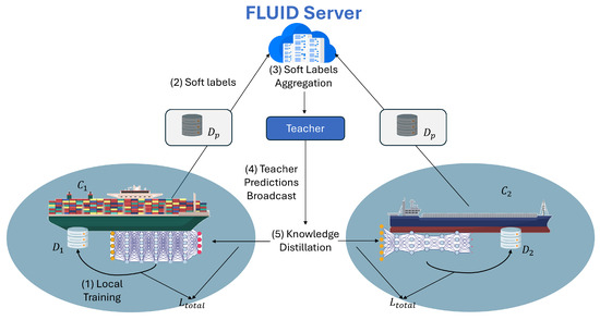
Figure 3. Detailed illustration of the FLUID KD process.

It should be noted that this reference dataset should be carefully curated to span the fleet’s operating regimes and periodically refined, as limited coverage (i.e., especially of rare faults) could lead to early saturation of distillation benefits. Specifically, each client i receives a local model variant ${\theta }_i$, tailored to its cluster and pruning level, trained on private data $D_i$, aimed at minimizing a combined loss:

$${\mathcal{L}}_i={\displaystyle \frac{1}{|D_i|}}\sum _{(x,y)\in D_i}{(f(x;{\theta }_i)-y)}^2+\lambda ·{\displaystyle \frac{1}{|D_{\mathrm{p}}|}}\sum _{x\in D_{\mathrm{p}}}{(f(x;{\theta }_i)-Z\left(x\right))}^2$$

(9)

where $f(x;{\theta }_i)$ is the client model’s raw output, y is the ground truth, $Z\left(x\right)$ is the ensemble teacher prediction on x, and $\lambda$ controls the strength of the distillation signal. After training, the client evaluates its updated model $D_{\mathrm{p}}$ and returns logits (pre-softmax soft label predictions):

$${\mathrm{logits}}_i\left(x\right)=f(x;{\theta }_i),\forall x\in D_{\mathrm{p}}.$$

(10)

After these steps, the server (i.e., teacher) aggregates the returned logits using weighted averaging:

$$Z\left(x\right)=\sum _{i\in \mathcal{S}}{\displaystyle \frac{n_i}{{\sum }_{j\in \mathcal{S}}{n}_j}}f(x;{\theta }_i).$$

(11)

This soft consensus forms the ensemble teacher Z, where $Z\left(x\right)$ is the teacher output and weights $n_i$ reflect the data volume at each client. Finally, teacher predictions are broadcast to all clients in the next round to guide their student training. This process enables the flexible participation, efficient bandwidth use, and compatibility across pruned and full-capacity ML model architectures (Algorithms 2 and 3).

Algorithm 2 FLUID: federated knowledge distillation loop (server side).

1: Input: Number of rounds R, initial teacher predictions $Z_{\mathrm{current}}\left(x\right)$   2: Phase 2: Iterative Federated Training   3: for round $t=1$ to R do   4:     Server selects a subset of active clients ${\mathcal{S}}_t$   5:     Initialize empty list: $L_{\mathrm{round}}\leftarrow \left[\right]$   6:     for each client $i\in {\mathcal{S}}_t$ (in parallel) do   7:         Send $Z_{\mathrm{current}}\left(x\right)$ to client i   8:                                                             \ Client executes Algorithm 3 and returns logits   9:         Receive $logit{s}_i\left(x\right)$ from client i 10:         Add $(logit{s}_i\left(x\right),n_i)$ to $L_{\mathrm{round}}$ 11:     end for 12:                                             \ Aggregate logits to update the global ensemble teacher 13:     $Z_{\mathrm{next}}\left(x\right)\leftarrow {\sum }_{(logit{s}_i,n_i)\in L_{\mathrm{round}}}{\displaystyle \frac{n_i}{{\sum }_j{n}_j}}·logit{s}_i\left(x\right)$ \ Weighted average (see Equation (11)) 14:     $Z_{\mathrm{current}}\left(x\right)\leftarrow Z_{\mathrm{next}}\left(x\right)$ 15: end for 16: return Final ensemble teacher $Z_{\mathrm{current}}\left(x\right)$

Algorithm 3 FLUID: client update procedure.

1: procedureClientUpdate($Z_{\mathrm{teacher}}$)   2:                    \ Model ${\theta }_{\mathrm{local}}$ was initialized via Algorithm 1 and persists across rounds.   3:     for epoch $=1$ to $E_{\mathrm{local}}$ do   4:                                                                                                          \ Train on private data   5:         for each batch $(x_b,y_b)\in D_{\mathrm{private}}$ do   6:            ${\mathcal{L}}_{\mathrm{private}}\leftarrow \mathrm{MSE}(f(x_b;{\theta }_{\mathrm{local}}),y_b)$   7:         end for   8:                                                                                          \ Calculate distillation loss   9:         for each batch $x_{p,b}\in D_{\mathrm{p}}$ do 10:            ${\mathcal{L}}_{\mathrm{distill}}\leftarrow \mathrm{MSE}(f(x_{p,b};{\theta }_{\mathrm{local}}),Z_{\mathrm{teacher}}\left(x_{p,b}\right))$ 11:         end for 12:                                                                           \ Combine losses and update model 13:         ${\mathcal{L}}_{\mathrm{total}}\leftarrow {\mathcal{L}}_{\mathrm{private}}+\lambda ·{\mathcal{L}}_{\mathrm{distill}}$ 14:         Update ${\theta }_{\mathrm{local}}$ using optimizer on $\nabla {\mathcal{L}}_{\mathrm{total}}$ 15:     end for 16:                                                                         \ Generate logits on the public dataset 17:     $logit{s}_{\mathrm{local}}\left(x\right)\leftarrow f(x;{\theta }_{\mathrm{local}})$ for all $x\in D_{\mathrm{p}}$ 18:     return $logit{s}_{\mathrm{local}}$ 19: end procedure

4. Experimental Setup

4.1. Dataset

For the development and assessment of the FLUID framework, we utilized an extended version of the dataset described in [23]. This dataset was gathered over a six-week voyage of a bulk carrier of Laskaridis Shipping Co., powered by a diesel ME (12,009HP), with a deadweight tonnage of 75,618 (DWT), and with a Westfalia OSD HFO purifier. In total, the dataset comprises 59,619 high-frequency time-series measurements spanning 759 distinct sensors distributed throughout the ship.

4.2. Data Preprocessing and Feature Engineering

For feature selection, a Pearson correlation test was performed on all measurements, identifying seven features with the strongest linear relationships, showcased in Table 1.

Table 1. Pressure and temperature features selected by Pearson correlation analysis.

Feature	Short Description
ME Lub Oil Inlet Pressure (bar)	Pressure of the lubricating oil, used to minimize friction and wear on engine parts
ME Air Spring Air Pressure (bar)	Compressed air pressure utilized to assist the pistons in transmitting power to the engine
ME Turbocharger Lub Oil Inlet Pressure (bar)	Pressure of the lubricating oil at the Turbocharger
DG Fuel Oil Inlet Pressure (bar)	Fuel oil pressure when entering the DG, used to check proper atomization and combustion performance
ME Fuel Oil Inlet Pressure (bar)	Fuel oil pressure when it enters the ME fuel system, affecting injection efficiency and combustion stability
ME Fuel Oil Inlet Temperature (°C)	Fuel oil temperature before entering the ME, influencing fuel viscosity and injection characteristics
ME Fuel Oil Outlet Temperature (°C)	Fuel oil temperature exiting the ME, reflecting heat exchange efficiency and thermal conditions of the fuel system

From these seven features, rows with NaN or non-coercible values were removed, resulting in discarding 2776 records in total. Furthermore, spectral feature extraction was performed to increase the model’s sensitivity in identifying machinery faults using the Time Series Feature Extraction Library (TSFEL) [56]. For each sensor window, the TSFEL computed 22 core spectral characteristics, including FFT mean coefficient, fundamental frequency, human range energy, LPCC, MFCC, Max power spectrum, Maximum frequency, Median frequency, Power bandwidth, and spectral features (centroid, decrease, distance, entropy, kurtosis, positive turning points, roll-off, roll-on, skewness, slope, spread, variation, and wavelet entropy). The analysis expanded our feature set to 525 dimensions, of which 13 exhibited zero variance across all windows and were therefore removed, leaving 512 for the final model inputs.

The remaining data were then normalized (min–max) to a range of [0, 1] to ensure that the magnitude of the value did not influence their importance. Finally, for the CML training scenario, the dataset was split into 80% training, 10% testing, and 10% validation. In the FL experiments, data splitting varied by method. For FedAvg, the dataset was evenly divided among four clients, while for both FLUID and FedAKD, 90% of the data were distributed equally across the clients (i.e., following again the 80/10/10 ratio for the local training), while the remaining 10% were allocated to the teacher model.

4.3. Baseline Model, Pruning Techniques, and Training Setup

To support the experiments in PdM, we adopt a modular two-stage architecture designed for feature compression and remaining useful life (RUL) estimation. This hybrid pipeline is representative of standard practices in time-series degradation modeling [23,57,58]. The architecture first uses a Convolutional AutoEncoder (CAE) to compress high-dimensional sensor sequences into informative latent embeddings. These features are then passed to a 1D-CNN predictor for regression. More specifically, inputs are treated as 1D sequences, while all Conv1D/Conv1DTranspose layers use the padding “same” and stride 1 (preserving sequence length) with ReLU nonlinearities. The CAE encoder comprises two Conv1D blocks with 64 and 32 filters (kernel size 3), each followed by dropout 0.1 and ReLU, with the resulting feature map being flattened and projected to a 64-dimensional latent vector via a Dense layer. The CAE decoder, first expands the latent with a Dense layer, and then applies two Conv1DTranspose layers with 64 and 1 filters (kernel size 3), using ReLU on the first and a linear activation at the output. For RUL estimation, a 1D-CNN predictor reshapes the latent as a short 1D sequence and applies two Conv1D layers with 128 (kernel 3) and 64 (kernel 1) filters, each followed by dropout 0.15 and ReLU, followed by a head consisting of Flatten and three Dense layers to produce the final estimation. The full model is trained end to end by using Mean Squared Error (MSE) and optimized via Adam with early stopping, while all network components use ReLU activations. In practice, the CAE is trained first to minimize reconstruction loss, while the predictor is trained subsequently using the CAE encoder’s output.

To support efficient model deployment across heterogeneous maritime clients, we evaluate multiple structured pruning strategies applied to the CNN predictor model. In detail, in this calibration phase, the uncompressed baseline model is trained on a resource-rich client (Tier L1) and subjected to two pruning methods:

• Polynomial Decay (PD): It gradually increases sparsity over training iterations, following a polynomial schedule [59,60].
• Constant Sparsity (CS): It applies a fixed sparsity ratio throughout training, providing stable compression [61,62].

To evaluate the performance of the proposed frameworks, we employed standard regression metrics. Specifically, we used the coefficient of determination $R^2$ to assess overall model fit, Mean Absolute Error (MAE) to quantify average prediction accuracy, and Root Mean Squared Error (RMSE) to capture the impact of larger prediction errors. To assess behavior under non-IID heterogeneity, we report MAE/RMSE both globally and per client, and summarize inter-client dispersion (mean ± SD) as a measure of fairness/stability across vessels. We also record CPU-based training time (s) to reflect deployability on resource-constrained ships.

5. Results

Simulations and algorithmic procedures ran on Python Google Compute Engine using the free-tier Collaboratory with 12.7 GB RAM, 107.7 GB Disk. The ML models were implemented using Python 3.11.0, TensorFlow library, version 2.12.0, TensorFlow Model Optimization, version 0.8.0, and TSFEL library, version 0.1.9, without GPU for model training acceleration.

5.1. Hyperparameter Tuning

We conducted series of experiments to identify the optimal values for all model and FL-related critical hyperparameters to run our setup. Specifically, for the CAE, we identified learning rate ${\eta }_1\in \{1\times {10}^{-4},\mathbf{5}\times {10}^{-4},1\times {10}^{-3},5\times {10}^{-3},1\times {10}^{-2}\}$ and batch size $|B_1|\in \{32,\mathbf{64},128\}$. Similarly, for the CNN, we set learning rate ${\eta }_2\in \{1\times {10}^{-4},\mathbf{2}\times {10}^{-4},1\times {10}^{-3},2\times {10}^{-3},1\times {10}^{-2}\}$, batch size $|B_2|\in \{32,\mathbf{64},128\}$, early stopping (ES) patience $P\in \{1,3,\mathbf{5},10,15\}$, and epochs $E\in \{100,150,\mathbf{300},350\}$. Concerning the different pruning strategies we used, PD sparsity $s_{\mathrm{PD}}\in [0.2,\mathbf{0}.\mathbf{3},0.4,\mathbf{0}.\mathbf{5},0.6,0.7]$, while CS $s_C\in [0.4,\mathbf{0}.\mathbf{5},0.6]$. Furthermore, the distillation coefficient $\alpha \in \{0.3,0.4,\mathbf{0}.\mathbf{5},0.6,0.8\}$, while the FL rounds $T\in \{150,\mathbf{300},350\}$, and the FL-round ES patience was set to $P_F\in \{1,\mathbf{5},10\}$.

5.2. Performance Analysis

After determining the optimal architecture and hyperparameters for the baseline PdM model, we trained and evaluated it under both centralized (CML) and federated (FL) settings. Following FLUID (Algorithm 1), the best available client was chosen. The model evaluated the different pruning methods, aiming to find the best method and its different hyperparameters to fit the remaining clusters (two in this case). Table 2 summarizes the results obtained using the full degradation dataset in the centralized setting, alongside the performance of the best-available client for local training under various pruning strategies with ES.

Table 2. Performance comparison of CML and best client.

Method	Model	MAE	RMSE	${\mathit{R}}^2$	Train Time (s)
CML	Baseline	0.03213	0.04379	0.97568	1307.76
	Polynomial Decay + ES	0.03489	0.04588	0.97331	271.65
	Constant Sparsity + ES	0.03747	0.04885	0.96974	373.79
Best Client	Baseline	0.03653	0.05516	0.96357	263.89
	Polynomial Decay (30%) + ES	0.06699	0.09023	0.90254	146.65
	Polynomial Decay (50%) + ES	0.06619	0.08873	0.90574	93.58
	Constant Sparsity + ES	0.07637	0.10416	0.87012	146.25

Specifically, the CML baseline model achieved the highest predictive accuracy but also required the longest training time. Furthermore, among the pruning approaches, PD was shown to consistently outperform CS-based pruning in both scenarios. Therefore, the client chose to further evaluate the different sparsing rates for PD (i.e., 30% and 50% in this case). Applying 30% and 50% PD pruning in the localized training scenario led to a significant degradation impact on $R^2$, which dropped to approximately 0.90, compared with the CML-trained model, while CS pruning further degraded performance to $R^2$ = 0.87. These results suggest that gradual weight removal via PD maintains predictive power more effectively than fixed-rate sparsification; nonetheless, when computational resources are not constrained, the centralized approach continues to offer the best overall performance. Figure 4 presents the training loss and the $R^2$ of the CML-trained model, while Figure 5 compares the predicted versus actual RUL values for the first 500 test samples.

Figure 4. CML-trained model results. (A) Evolution of training and validation loss for the baseline model. (B) Actual and predicted values of the testing samples of HFO RUL degradation, where the dashed line represents the ideal "actual vs. predicted" matching $(y=x)$. Validation curves: (C) shows the CS-driven losses and (D) the PD-driven losses.

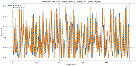
Figure 5. CML-trained baseline models predictive performance analysis against the actual RUL values for the first 500 samples.

After identifying the optimal pruning schedules via PD for the individual clients, we applied these configurations across multiple cluster settings to evaluate FLUID in both controlled and realistic FL scenarios, as showcased in Table 3. Specifically, a sensitivity study was conducted, evaluating FLUID against strong FL baselines, including FedAvg and FedAKD, as well as under different cluster settings, (i) uniform 30% pruning to all clients, (ii) uniform 50% to all clients, and (iii) mixed-tier 0%/30%/50% pruning, to cover both controlled and realistic fleet scenarios.

Table 3. Performance comparison of FL methods.

Method	Prune	KD	Global MAE	Global RMSE	Global ${\mathit{R}}^2$	Train (s)	Mean MAEc (±SD)	Mean RMSEc (±SD)
FedAvg [11]	0	✗	0.04335	0.07215	0.9398	1764.23	0.03957(28)	0.05258(56)
FedAKD [20]	0	✓	0.05387	0.08318	0.9199	1820.75	0.02639(23)	0.04229(32)
FLUID	30	✓	0.04647	0.06784	0.9468	3774.65	0.02557(21)	0.04182(28)
	50	✓	0.04917	0.07525	0.9345	3026.98	0.02694(21)	0.04294(33)
	0–50 *	✓	0.04727	0.07482	0.9352	4102.31	0.02575(21)	0.04190(36)

* Four clients, each with a different pruned model: 1 × 0%, 1 × 30%, and 2 × 50%.

Our results indicate that FedAvg, despite its lower training cost, underperforms all KD-based variants both globally and at the client level. FedAKD improves over FedAvg by leveraging KD, but its single-cluster design limits its overall accuracy. In contrast, the FLUID variant with uniform distribution of 30% sparsity across the clients achieved both the highest global scores and the lowest mean error per client. Similarly, the variant with 50% uniform sparsity models trained at weaker resource clients remained competitive, despite having half of their weights pruned, with minimal performance degradation based on mean client performance. Moreover, the mixed-sparsity deployment scenario, where different sparsity levels are applied, to better reflect real-world conditions, yielded an RMSE_c of 0.04190 ± 0.0036, showing that FLUID can effectively adapt to heterogeneous client capabilities, only at the cost of higher training time. Notably, across both uniform sparsity settings (K = 1, where 30% and 50% are applied), FLUID maintained consistent per-client MAE scores of approximately 0.025–0.027 with very small standard deviations at around 0.021. Even in the realistic mixed-cluster heterogeneous model deployment scenario (K = 3, with clients having models with 1×0%, 1×30%, and 2×50% sparsity levels), the mean MAE_c remained at 0.02575 ± 0.021. This stability shows that no single client suffers even when some clients prune half their models, thus demonstrating robustness to model heterogeneity.

Figure 6 showcases the global validation loss over federated rounds for FedAvg, FedAKD, and FLUID (K = 3 mixed-sparsity configuration). Notably, all methods exhibit a rapid decrease in loss within the first five rounds. FedAvg achieves the lowest steady-state loss (around 0.0040), while FLUID converges nearly as quickly to a slightly higher plateau (0.0045–0.0050). In contrast, FedAKD stabilized more slowly and at a higher loss level (0.0052–0.0056). Furthermore, a closer look at rounds 10–50 reveals that FLUID maintains convergence within 10–20% of FedAvg’s final loss while outperforming FedAKD. However, this comes at the cost of longer training, as FLUID requires roughly 2–3× more rounds than FedAvg and exhibits marginally more fluctuation around its plateau. These results indicate that FLUID’s dynamic pruning nearly preserves FedAvg’s convergence speed and stability, offering a trade-off between model accuracy and communication/computation efficiency.

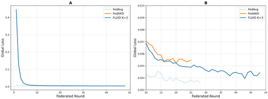
Figure 6. Global validation loss for FedAvg, FedAKD, and FLUID K = 3 per FL round. (A) Validation loss of the proposed methodologies across their FL rounds. (B) Detailed view of rounds 10–50.

6. Discussion

While our study focuses on RUL prediction for an HFO purifier, FLUID can be extended to other PdM systems targeting dynamic marine equipment and machinery, enabling participation even by low-resource vessels.

Our results demonstrate that FLUID’s integration of dynamic structured pruning and logit-based knowledge distillation produces models that are both computationally efficient and highly accurate across heterogeneous, resource-constrained clients.

In detail, FLUID’s calibration module and pruning--distribution protocol are agnostic to the specific sparsity criterion. While we adopted a PD schedule, potential users can also utilize alternative methods, such as $L_1$-norm [63,64] or $L_2$-norm magnitude pruning [65,66], channel pruning heuristics [67,68], or even learned sparsity masks, to suit different architectures and data characteristics. The frameworks calibration phase will identify the optimal schedules and sparsity levels for any chosen method, aligning with other works that have observed that pruning norms yield distinct accuracy–efficiency trade-offs depending on network depth and redundancy [69,70].

Furthermore, in CML benchmarks, higher sparsity levels (e.g., 50%) under PD incur only marginal accuracy drops ($R^2$ around 0.969 vs. 0.973 for the dense model), consistent with findings that gradual sparsification preserves performance better than abrupt weight removal. However, in federated deployment, heavier pruning amplifies gradient noise across non-IID clients and slows convergence. Specifically, 50% PD achieved a global $R^2$ of 0.934, whereas 30% PD yielded 0.9468. This divergence highlights that pruning optima in CML do not always transfer to FL [71]. FLUID’s calibration mechanism makes these distinctions explicit, but practitioners should re-evaluate sparsity levels when migrating to new scenarios.

Prior works, such as FedAKD and FedDF have shown that soft-logit aggregation alleviates both architectural heterogeneity and privacy concerns inherent in raw-weight sharing [20,52]. Our experimental results further confirm these insights, as distillation showcases to not only harmonize updates among pruned and unpruned architectures but also compensates for the information loss due to compression. In addition, FLUID further advances this paradigm by tightly coupling distillation with client-aware pruning while maintaining or even improving predictive accuracy in some cases.

Concerning the limitations and future research directions of this work, there are multiple routes to explore. In detail, while FLUID reduces raw-weight exchange, soft logits can inadvertently leak sensitive information about local data distributions [72]. Future work should integrate defenses such as differential privacy, secure multi-party computation, or gradient obfuscation tailored to logit aggregation. Research efforts should also evaluate the effect of FLUID’s dynamic pruning on robustness against adversarial attacks, including both gradient-based and query-based threat models, and explore pruning schedules that explicitly regularize for robustness. Additionally, clients may vary not only in memory but also in FLOPs, energy consumption, and runtime latency. Incorporating real-time profiling and cost-aware pruning criteria (e.g., optimizing under a FLOP budget) will further refine FLUID’s adaptability to diverse hardware constraints. Another critical challenge lies with FLUID’s scalability. Our evaluation employed a small number of clients with curated non-IID splits. Scaling FLUID to potentially hundreds or thousands of devices with varied connectivity patterns, failure modes, and data distribution will require advanced client scheduling and selection policies, fault tolerance, and possibly asynchronous or partial-update federated distillation protocols. Moreover, as real-world satellite and edge networks exhibit fluctuating latency and bandwidth, a challenge lies in adapting the pruning schedules and distillation frequencies to real-time network metrics or employing the delta encoding of logits, which could optimize communication efficiency under volatile conditions.

7. Conclusions

Overall, FLUID enables fleet-wide inclusion, as every vessel can train and deploy a PdM model sized to its onboard resources, while all models remain interoperable through prediction-space aggregation over a small reference set. This design avoids the common pitfall of excluding low-resource clients and reduces blind spots in fleet monitoring. By unifying dynamic pruning with federated distillation, FLUID offers a practical path toward privacy-preserving, efficient, and accurate edge-computing solutions. Addressing the outlined research challenges will further strengthen its applicability to large-scale, heterogeneous Federated Learning deployment across industry domains.

References

- Achouch, M.; Dimitrova, M.; Ziane, K.; Sattarpanah Karganroudi, S.; Dhouib, R.; Ibrahim, H.; Adda, M. On predictive maintenance in industry 4.0: Overview, models, and challenges. Appl. Sci. 2022, 12, 8081. [Google Scholar] [CrossRef]
- Makridis, G.; Kyriazis, D.; Plitsos, S. Predictive maintenance leveraging machine learning for time-series forecasting in the maritime industry. In Proceedings of the 2020 IEEE 23rd International Conference on Intelligent Transportation Systems (ITSC), Rhodes, Greece, 20–23 September 2020; pp. 1–8. [Google Scholar]
- Han, X.; Wang, Z.; Xie, M.; He, Y.; Li, Y.; Wang, W. Remaining useful life prediction and predictive maintenance strategies for multi-state manufacturing systems considering functional dependence. Reliab. Eng. Syst. Saf. 2021, 210, 107560. [Google Scholar] [CrossRef]
- Mitici, M.; de Pater, I.; Barros, A.; Zeng, Z. Dynamic predictive maintenance for multiple components using data-driven probabilistic RUL prognostics: The case of turbofan engines. Reliab. Eng. Syst. Saf. 2023, 234, 109199. [Google Scholar] [CrossRef]
- Bemani, A.; Björsell, N. Aggregation strategy on federated machine learning algorithm for collaborative predictive maintenance. Sensors 2022, 22, 6252. [Google Scholar] [CrossRef] [PubMed]
- Kalafatelis, A.S.; Nomikos, N.; Giannopoulos, A.; Alexandridis, G.; Karditsa, A.; Trakadas, P. Towards predictive maintenance in the maritime industry: A component-based overview. J. Mar. Sci. Eng. 2025, 13, 425. [Google Scholar] [CrossRef]
- Huang, Y.; Liu, W.; Lin, Y.; Kang, J.; Zhu, F.; Wang, F.Y. FLCSDet: Federated learning-driven cross-spatial vessel detection for maritime surveillance with privacy preservation. IEEE Trans. Intell. Transp. Syst. 2024, 26, 1177–1192. [Google Scholar] [CrossRef]
- Imteaj, A.; Mamun Ahmed, K.; Thakker, U.; Wang, S.; Li, J.; Amini, M.H. Federated learning for resource-constrained iot devices: Panoramas and state of the art. In Federated and Transfer Learning; Springer: Cham, Switzerland, 2022; pp. 7–27. [Google Scholar]
- Imteaj, A.; Thakker, U.; Wang, S.; Li, J.; Amini, M.H. A survey on federated learning for resource-constrained IoT devices. IEEE Internet Things J. 2021, 9, 1–24. [Google Scholar] [CrossRef]
- Imteaj, A.; Amini, M.H. FedPARL: Client activity and resource-oriented lightweight federated learning model for resource-constrained heterogeneous IoT environment. Front. Commun. Netw. 2021, 2, 657653. [Google Scholar] [CrossRef]
- McMahan, B.; Moore, E.; Ramage, D.; Hampson, S.; y Arcas, B.A. Communication-efficient learning of deep networks from decentralized data. In Proceedings of the Artificial Intelligence and Statistics, Fort Lauderdale, FL, USA, 20–22 April 2017; pp. 1273–1282. [Google Scholar]
- Li, T.; Sahu, A.K.; Zaheer, M.; Sanjabi, M.; Talwalkar, A.; Smith, V. Federated optimization in heterogeneous networks. Proc. Mach. Learn. Syst. 2020, 2, 429–450. [Google Scholar]
- Ye, M.; Fang, X.; Du, B.; Yuen, P.C.; Tao, D. Heterogeneous federated learning: State-of-the-art and research challenges. ACM Comput. Surv. 2023, 56, 1–44. [Google Scholar] [CrossRef]
- Fan, B.; Jiang, S.; Su, X.; Tarkoma, S.; Hui, P. A survey on model-heterogeneous federated learning: Problems, methods, and prospects. In Proceedings of the 2024 IEEE International Conference on Big Data (BigData), Washington, DC, USA, 15–18 December 2024; pp. 7725–7734. [Google Scholar]
- Li, W.; Li, T. Comparison of deep learning models for predictive maintenance in industrial manufacturing systems using sensor data. Sci. Rep. 2025, 15, 23545. [Google Scholar] [CrossRef]
- Qi, P.; Chiaro, D.; Piccialli, F. Small models, big impact: A review on the power of lightweight Federated Learning. Future Gener. Comput. Syst. 2025, 162, 107484. [Google Scholar] [CrossRef]
- Hinton, G.; Vinyals, O.; Dean, J. Distilling the knowledge in a neural network. arXiv 2015, arXiv:1503.02531. [Google Scholar] [CrossRef]
- Gou, J.; Yu, B.; Maybank, S.J.; Tao, D. Knowledge distillation: A survey. Int. J. Comput. Vis. 2021, 129, 1789–1819. [Google Scholar] [CrossRef]
- Wu, C.; Wu, F.; Lyu, L.; Huang, Y.; Xie, X. Communication-efficient federated learning via knowledge distillation. Nat. Commun. 2022, 13, 2032. [Google Scholar] [CrossRef] [PubMed]
- Gad, G.; Fadlullah, Z. Federated learning via augmented knowledge distillation for heterogenous deep human activity recognition systems. Sensors 2022, 23, 6. [Google Scholar] [CrossRef]
- Li, D.; Wang, J. Fedmd: Heterogenous federated learning via model distillation. arXiv 2019, arXiv:1910.03581. [Google Scholar] [CrossRef]
- Foretich, A.; Zaimes, G.G.; Hawkins, T.R.; Newes, E. Challenges and opportunities for alternative fuels in the maritime sector. Marit. Transp. Res. 2021, 2, 100033. [Google Scholar] [CrossRef]
- Kalafatelis, A.S.; Stamou, N.; Dailani, A.; Theodoridis, T.; Nomikos, N.; Giannopoulos, A.; Tsoulakos, N.; Alexandridis, G.; Trakadas, P. A Lightweight Predictive Maintenance Strategy for Marine HFO Purification Systems. In Proceedings of the European, Mediterranean, and Middle Eastern Conference on Information Systems, Athens, Greece, 2–3 September 2024; pp. 88–99. [Google Scholar]
- Başhan, V.; Demirel, H.; Celik, E. Evaluation of critical problems of heavy fuel oil separators on ships by best-worst method. Proc. Inst. Mech. Eng. Part M J. Eng. Marit. Environ. 2022, 236, 868–876. [Google Scholar] [CrossRef]
- Kandemir, Ç.; Çelik, M.; Akyuz, E.; Aydin, O. Application of human reliability analysis to repair & maintenance operations on-board ships: The case of HFO purifier overhauling. Appl. Ocean. Res. 2019, 88, 317–325. [Google Scholar]
- Ayvaz, S.; Karakurt, A. Examination of Failures in the Marine Fuel and Lube Oil Separators Through the Fuzzy DEMATEL Method. J. ETA Marit. Sci. 2025, 13, 36–45. [Google Scholar] [CrossRef]
- Han, P.; Ellefsen, A.L.; Li, G.; Æsøy, V.; Zhang, H. Fault prognostics using LSTM networks: Application to marine diesel engine. IEEE Sens. J. 2021, 21, 25986–25994. [Google Scholar] [CrossRef]
- Gribbestad, M.; Hassan, M.U.; Hameed, I.A. Transfer learning for Prognostics and health Management (PHM) of marine Air Compressors. J. Mar. Sci. Eng. 2021, 9, 47. [Google Scholar] [CrossRef]
- Tang, W.; Roman, D.; Dickie, R.; Robu, V.; Flynn, D. Prognostics and health management for the optimization of marine hybrid energy systems. Energies 2020, 13, 4676. [Google Scholar] [CrossRef]
- Liu, B.; Gan, H.; Chen, D.; Shu, Z. Research on fault early warning of marine diesel engine based on CNN-BiGRU. J. Mar. Sci. Eng. 2022, 11, 56. [Google Scholar] [CrossRef]
- Wu, J.Y.; Wu, M.; Chen, Z.; Li, X.L.; Yan, R. Degradation-aware remaining useful life prediction with LSTM autoencoder. IEEE Trans. Instrum. Meas. 2021, 70, 1–10. [Google Scholar] [CrossRef]
- Angelopoulos, A.; Giannopoulos, A.; Nomikos, N.; Kalafatelis, A.; Hatziefremidis, A.; Trakadas, P. Federated learning-aided prognostics in the shipping 4.0: Principles, workflow, and use cases. IEEE Access 2024, 12, 6437–6454. [Google Scholar] [CrossRef]
- Giannopoulos, A.E.; Spantideas, S.T.; Zetas, M.; Nomikos, N.; Trakadas, P. Fedship: Federated over-the-air learning for communication-efficient and privacy-aware smart shipping in 6g communications. IEEE Trans. Intell. Transp. Syst. 2024. [Google Scholar] [CrossRef]
- Abreha, H.G.; Hayajneh, M.; Serhani, M.A. Federated learning in edge computing: A systematic survey. Sensors 2022, 22, 450. [Google Scholar] [CrossRef] [PubMed]
- Hohman, F.; Kery, M.B.; Ren, D.; Moritz, D. Model compression in practice: Lessons learned from practitioners creating on-device machine learning experiences. In Proceedings of the 2024 CHI Conference on Human Factors in Computing Systems, Honolulu, HI, USA, 11–16 May 2024; pp. 1–18. [Google Scholar]
- Kalafatelis, A.S.; Nomikos, N.; Giannopoulos, A.; Trakadas, P. A Survey on Predictive Maintenance in the Maritime Industry Using Machine and Federated Learning. Authorea Prepr. 2024, 1–30. [Google Scholar]
- Zhang, C.; Xie, Y.; Bai, H.; Yu, B.; Li, W.; Gao, Y. A survey on federated learning. Knowl.-Based Syst. 2021, 216, 106775. [Google Scholar] [CrossRef]
- Wen, J.; Zhang, Z.; Lan, Y.; Cui, Z.; Cai, J.; Zhang, W. A survey on federated learning: Challenges and applications. Int. J. Mach. Learn. Cybern. 2023, 14, 513–535. [Google Scholar] [CrossRef]
- Wang, J.; Liu, Q.; Liang, H.; Joshi, G.; Poor, H.V. Tackling the objective inconsistency problem in heterogeneous federated optimization. Adv. Neural Inf. Process. Syst. 2020, 33, 7611–7623. [Google Scholar]
- Karimireddy, S.P.; Kale, S.; Mohri, M.; Reddi, S.; Stich, S.; Suresh, A.T. Scaffold: Stochastic controlled averaging for federated learning. In Proceedings of the International Conference on Machine Learning, Virtual, 13–18 July 2020; pp. 5132–5143. [Google Scholar]
- Nguyen, D.P.; Yu, S.; Muñoz, J.P.; Jannesari, A. Enhancing heterogeneous federated learning with knowledge extraction and multi-model fusion. In Proceedings of the SC’23 Workshops of the International Conference on High Performance Computing, Network, Storage, and Analysis, Denver, CO, USA, 12–17 November 2023; pp. 36–43. [Google Scholar]
- Han, S.; Pool, J.; Tran, J.; Dally, W. Learning both weights and connections for efficient neural network. Adv. Neural Inf. Process. Syst. 2015, 28. [Google Scholar]
- Li, H.; Kadav, A.; Durdanovic, I.; Samet, H.; Graf, H.P. Pruning filters for efficient convnets. arXiv 2016, arXiv:1608.08710. [Google Scholar]
- Jiang, Y.; Wang, S.; Valls, V.; Ko, B.J.; Lee, W.H.; Leung, K.K.; Tassiulas, L. Model pruning enables efficient federated learning on edge devices. IEEE Trans. Neural Netw. Learn. Syst. 2022, 34, 10374–10386. [Google Scholar] [CrossRef]
- Xu, W.; Fang, W.; Ding, Y.; Zou, M.; Xiong, N. Accelerating federated learning for iot in big data analytics with pruning, quantization and selective updating. IEEE Access 2021, 9, 38457–38466. [Google Scholar] [CrossRef]
- Huang, H.; Zhuang, W.; Chen, C.; Lyu, L. Fedmef: Towards memory-efficient federated dynamic pruning. In Proceedings of the IEEE/CVF Conference on Computer Vision and Pattern Recognition, Seattle, WA, USA, 16–22 June 2024; pp. 27548–27557. [Google Scholar]
- Zhou, G.; Xu, K.; Li, Q.; Liu, Y.; Zhao, Y. AdaptCL: Efficient collaborative learning with dynamic and adaptive pruning. arXiv 2021, arXiv:2106.14126. [Google Scholar] [CrossRef]
- Internò, C.; Raponi, E.; van Stein, N.; Bäck, T.; Olhofer, M.; Jin, Y.; Hammer, B. Adaptive hybrid model pruning in federated learning through loss exploration. In Proceedings of the International Workshop on Federated Foundation Models in Conjunction with NeurIPS 2024, Vancouver, BC, Canada, 15 December 2024. [Google Scholar]
- Buciluǎ, C.; Caruana, R.; Niculescu-Mizil, A. Model compression. In Proceedings of the 12th ACM SIGKDD International Conference on Knowledge Discovery and Data Mining, Philadelphia, PA, USA, 20–23 August 2006; pp. 535–541. [Google Scholar]
- Fukuda, T.; Suzuki, M.; Kurata, G.; Thomas, S.; Cui, J.; Ramabhadran, B. Efficient knowledge distillation from an ensemble of teachers. In Proceedings of the Interspeech, Stockholm, Sweden, 20–24 August 2017; pp. 3697–3701. [Google Scholar]
- Lan, L.; Zhu, X.; Gong, S. Knowledge distillation by on-the-fly native ensemble. Adv. Neural Inf. Process. Syst. 2018, 31. [Google Scholar]
- Lin, T.; Kong, L.; Stich, S.U.; Jaggi, M. Ensemble distillation for robust model fusion in federated learning. Adv. Neural Inf. Process. Syst. 2020, 33, 2351–2363. [Google Scholar]
- Afonin, A.; Karimireddy, S.P. Towards model agnostic federated learning using knowledge distillation. arXiv 2021, arXiv:2110.15210. [Google Scholar]
- Kang, H.; Cha, S.; Kang, J. GeFL: Model-Agnostic Federated Learning with Generative Models. arXiv 2024, arXiv:2412.18460. [Google Scholar] [CrossRef]
- Shin, Y.; Lee, K.; Lee, S.; Choi, Y.R.; Kim, H.S.; Ko, J. Effective heterogeneous federated learning via efficient hypernetwork-based weight generation. In Proceedings of the 22nd ACM Conference on Embedded Networked Sensor Systems, Hangzhou, China, 4–7 November 2024; pp. 112–125. [Google Scholar]
- Barandas, M.; Folgado, D.; Fernandes, L.; Santos, S.; Abreu, M.; Bota, P.; Liu, H.; Schultz, T.; Gamboa, H. TSFEL: Time series feature extraction library. SoftwareX 2020, 11, 100456. [Google Scholar] [CrossRef]
- Bosello, M.; Falcomer, C.; Rossi, C.; Pau, G. To charge or to sell? EV pack useful life estimation via LSTMs, CNNs, and autoencoders. Energies 2023, 16, 2837. [Google Scholar] [CrossRef]
- Ji, Z.; Gan, H.; Liu, B. A deep learning-based fault warning model for exhaust temperature prediction and fault warning of marine diesel engine. J. Mar. Sci. Eng. 2023, 11, 1509. [Google Scholar] [CrossRef]
- Bird, J.J.; Barnes, C.M.; Manso, L.J.; Ekárt, A.; Faria, D.R. Fruit quality and defect image classification with conditional GAN data augmentation. Sci. Hortic. 2022, 293, 110684. [Google Scholar] [CrossRef]
- Zhu, M.; Gupta, S. To prune, or not to prune: Exploring the efficacy of pruning for model compression. arXiv 2017, arXiv:1710.01878. [Google Scholar] [CrossRef]
- Hoefler, T.; Alistarh, D.; Ben-Nun, T.; Dryden, N.; Peste, A. Sparsity in deep learning: Pruning and growth for efficient inference and training in neural networks. J. Mach. Learn. Res. 2021, 22, 1–124. [Google Scholar]
- Jayakumar, S.; Pascanu, R.; Rae, J.; Osindero, S.; Elsen, E. Top-kast: Top-k always sparse training. Adv. Neural Inf. Process. Syst. 2020, 33, 20744–20754. [Google Scholar]
- Ma, R.; Miao, J.; Niu, L.; Zhang, P. Transformed ℓ1 regularization for learning sparse deep neural networks. Neural Netw. 2019, 119, 286–298. [Google Scholar] [CrossRef]
- Collins, M.D.; Kohli, P. Memory bounded deep convolutional networks. arXiv 2014, arXiv:1412.1442. [Google Scholar] [CrossRef]
- Idelbayev, Y.; Carreira-Perpinán, M.A. Exploring the Effect of ℓ0/ℓ2 Regularization in Neural Network Pruning using the LC Toolkit. In Proceedings of the ICASSP 2022 IEEE International Conference on Acoustics, Speech and Signal Processing (ICASSP), Singapore, 22–27 May 2022; pp. 3373–3377. [Google Scholar]
- Jacot, A.; Golikov, E.; Hongler, C.; Gabriel, F. Feature Learning in L_2-regularized DNNs: Attraction/Repulsion and Sparsity. Adv. Neural Inf. Process. Syst. 2022, 35, 6763–6774. [Google Scholar]
- Chen, Y.; Wang, Z. An effective information theoretic framework for channel pruning. arXiv 2024, arXiv:2408.16772. [Google Scholar]
- Liu, Y.; Wu, D.; Zhou, W.; Fan, K.; Zhou, Z. EACP: An effective automatic channel pruning for neural networks. Neurocomputing 2023, 526, 131–142. [Google Scholar] [CrossRef]
- Pons, I.; Yamamoto, B.; Reali Costa, A.H.; Jordao, A. Effective layer pruning through similarity metric perspective. In Proceedings of the International Conference on Pattern Recognition, Kolkata, India, 1–5 December 2024; pp. 423–438. [Google Scholar]
- Marinó, G.C.; Petrini, A.; Malchiodi, D.; Frasca, M. Deep neural networks compression: A comparative survey and choice recommendations. Neurocomputing 2023, 520, 152–170. [Google Scholar] [CrossRef]
- Internò, C.; Raponi, E.; van Stein, N.; Bäck, T.; Olhofer, M.; Jin, Y.; Hammer, B. Automated Federated Learning via Informed Pruning. arXiv 2024, arXiv:2405.10271v1. [Google Scholar] [CrossRef]
- Shao, J.; Li, Z.; Sun, W.; Zhou, T.; Sun, Y.; Liu, L.; Lin, Z.; Mao, Y.; Zhang, J. A survey of what to share in federated learning: Perspectives on model utility, privacy leakage, and communication efficiency. arXiv 2023, arXiv:2307.10655. [Google Scholar]
Disclaimer/Publisher’s Note: The statements, opinions and data contained in all publications are solely those of the individual author(s) and contributor(s) and not of MDPI and/or the editor(s). MDPI and/or the editor(s) disclaim responsibility for any injury to people or property resulting from any ideas, methods, instructions or products referred to in the content. |
© 2025 by the authors. Licensee MDPI, Basel, Switzerland. This article is an open access article distributed under the terms and conditions of the Creative Commons Attribution (CC BY) license (https://creativecommons.org/licenses/by/4.0/).