Abstract
Screw propulsors have attracted increasing attention for their potential applications in amphibious vehicles and benthic robots, owing to their ability to perform both terrestrial and underwater locomotion. To investigate their hydrodynamic characteristics, a two-stage numerical analysis was carried out. In the first stage, steady-state simulations under various advance coefficients were conducted to evaluate the influence of key geometric parameters on propulsion performance. Based on these results, a representative configuration was then selected for transient analysis to capture unsteady flow features. In the second stage, a Detached Eddy Simulation approach was employed to capture unsteady flow features under three rotational speeds. The flow field information was analyzed, and the mechanisms of vortex generation, instability, and dissipation were comprehensively studied. The results reveal that the propulsion process is dominated by the formation and evolution of tip vortices, root vortices, and cylindrical wake vortices. As rotation speed increases, vortex structures exhibit a transition from ordered spiral wakes to chaotic turbulence, primarily driven by centrifugal instability and nonlinear vortex interactions. Vortex breakdown and energy dissipation are intensified downstream, especially under high-speed conditions, where vortex integrity is rapidly lost due to strong shear and radial expansion. This hydrodynamic behavior highlights the fundamental difference from conventional propellers, and these findings provide theoretical insight into the flow mechanisms of screw propulsion.
1. Introduction
The screw propulsor has garnered increasing attention in the fields of amphibious robotics and underwater vehicles. Unlike conventional propellers that are primarily suited for open-water navigation, screw propulsion systems exhibit inherent adaptability to complex terrains, including mud, sand, and submerged surfaces. This makes them particularly advantageous for amphibious vehicles operating in coastal zones, intertidal environments, or benthic exploration missions. In recent years, several engineering prototypes and field-deployed vehicles have adopted screw propulsors to fulfill multi-environmental locomotion requirements. Figure 1 illustrates a range of robotic systems employing screw propulsion across different engineering applications. Among these, the screw propulsors inspired by biological locomotion and space screw drive mechanisms offer a promising alternative to conventional propellers, especially in shallow water, ice, snow, complex terrain, or amphibious operations [1].
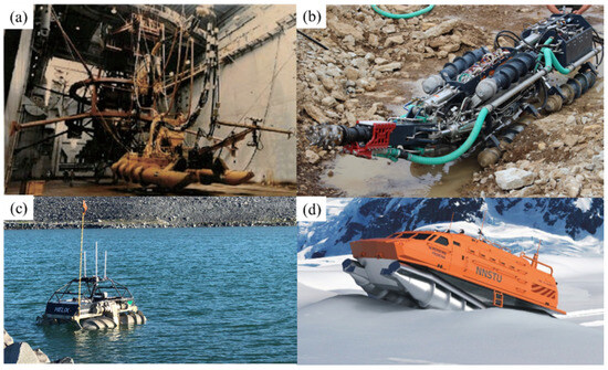
Figure 1.
Representative applications of screw propulsion in amphibious and seabed vehicles. (a) The Archimedes spiral mining robot developed by the Ocean Mining Company (OMCO) of the United States successfully collected nodules from the seabed at a depth of 4877 m in the Pacific Ocean [2]. (b) The final prototype of the ROBOMINERS project [3]. The robot with screw propulsion is suitable for traveling in mining areas, which are flooded, have complex terrain, and are difficult to exploit. (c) HELIX Neptune—amphibious robot [4]. A robotic platform specifically for environmental monitoring that can collect data and water samples from hazardous locations. (d) The universal rescue rotary-screw vehicle (URV) for the Arctic region is being developed at the NNSTU named after R.E. Alekseev [5], which can be used to rescue people in distress in the Arctic region and the Far North.
Our team has developed an amphibious unmanned vehicle named CSUB, which has been successfully applied in coastal zone missions such as environmental monitoring and terrain investigation. Based on this technological foundation, we are currently advancing toward the development of next-generation platforms with benthic locomotion capabilities for deep-sea operations. Figure 2 illustrates the development roadmap of our work, progressing from coastal missions to subaqueous operations. As the operational scenarios expand from coastal zones to benthic regions, understanding the hydrodynamic behavior of screw propulsors becomes increasingly essential. Therefore, a detailed investigation into the flow mechanisms is necessary.
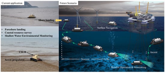
Figure 2.
Present capabilities and prospective deployment scenarios of our autonomous screw-driven vehicles.
Despite their practical appeal, the hydrodynamic performance of screw propulsors remains poorly understood, and there is very little publicly available data on this matter. Their propulsion efficiency is generally inferior to that of conventional propellers [6]. However, understanding the nature of these flow structures is essential for evaluating performance and guiding optimization. Previous studies have mainly focused on the geometric design or mechanical characteristics of the screw propulsor, while systematic investigations of their flow field structure and vortex dynamics remain limited [7]. Gao et al. [8] conducted numerical simulations to analyze the propulsive performance of a screw-propelled inspection robot, focusing on the effects of the parameter count on propulsion efficiency and motion stability. However, the study primarily addressed overall performance metrics without further investigating the underlying flow mechanisms or transient hydrodynamic behaviors. Zhu et al. [9] investigated the underwater propulsion performance of Archimedean screws under mooring conditions, focusing on the effects of key dimensionless geometric parameters. While their study provides valuable guidance for design optimization, it lacks a detailed exploration of how operational parameters influence unsteady flow structures and hydrodynamic efficiency. Donohue et al. [10] conducted simulations to study the underwater propulsion of a screw propulsor for an amphibious rover, but the work lacks detailed analysis of the surrounding flow field.
To accurately capture the complex hydrodynamic behavior of screw propulsion, various numerical methods have been employed, with Computational Fluid Dynamics (CFD). The Reynolds-Averaged Navier–Stokes (RANS) solver enjoys much popularity in engineering applications, due to its acceptable accuracy and the few computation resources it requires. Ji et al. [11] utilized the Shear Stress Transport (SST) turbulence model to investigate the flow around a propeller. The RANS model often overestimates turbulent viscosity, and due to its Reynolds-averaged approach, fails to capture the unsteady nature of real flow. Consequently, there is a growing preference for Large Eddy Simulation (LES) because of its higher accuracy in resolving transient flow structures [12]. Despite the high fidelity of the LES method, its significant computational demand limits its practical application, especially for full-scale or long-duration simulations [13]. To balance accuracy and efficiency, the Delayed Detached Eddy Simulation (DDES) method has been developed, combining the strengths of RANS and LES approaches. DDES employs RANS modeling near walls to reduce computational cost while switching to LES in separated regions to capture large-scale turbulence. Lu et al. [14] compared RANS and DDES in simulating propeller flow under four-quadrant conditions, showing that, while RANS suffices for aligned flows, DDES better captures complex vortex dynamics and force accuracy in opposing flow scenarios.
Therefore, in this study, a comprehensive numerical investigation was conducted to explore the hydrodynamic characteristics of screw propulsors, which remain under explored compared to conventional marine propellers. A two-stage simulation framework was adopted, combining steady-state and unsteady analyses. In the first stage, steady-state RANS simulations were conducted to systematically examine the effects of key geometric parameters on propulsion performance across different advance ratios. Based on the findings, a representative configuration was selected for transient analysis using the DDES method.
Due to the lack of research on detailed flow field analyses of screw propulsors, this study provides a refined investigation into the internal flow structures, capturing key vortex phenomena such as generation, pairing, deformation, and breakdown. These observations help explain the inherent flow instability and momentum diffusion associated with this type of propulsion. The results not only deepen the understanding of its unsteady vortex dynamics but also contribute to the theoretical foundation for future optimization and design improvements.
2. Geometric Design Space and Operating Conditions
2.1. Geometric Design Space
In this study, the screw propulsors with different parameters were considered to investigate the hydrodynamic performance under various advance coefficients. The critical design parameters of a screw propulsor are displayed in Figure 3. L is the overall length, is the helix angle, D is the outer screw diameter, d is the base cylinder diameter.
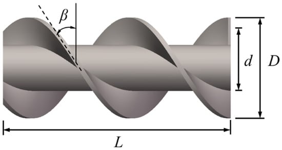
Figure 3.
Geometry parameters of the screw propulsor.
The geometric design space was constructed based on two key geometric variables: the diameter ratio and helix angle , where is equal to the base cylinder diameter d divided by the outer screw diameter D. The base cylinder diameter d and overall length were kept constant as 100 mm and 400 mm. The parameter combinations and their respective values are summarized in Table 1.

Table 1.
Parametric design configurations.
2.2. Operation Conditions
In order to assess the hydrodynamic performance of each parameter combination, the characteristics need to be quantified. This follows the traditional propulsive efficiency analysis method [15]. The advanced ratio J is defined in Equation (1).
where N is the rotational speed and is the free stream velocity. For each advance ratio, the torque coefficient and thrust coefficient are defined in Equation (2).
Here, Q is the torque (N·m), T is the thrust, and is the water density (kg/m3). The hydrodynamic efficiency was selected as the quantitative basis and is defined in Equation (3).
Two sets of hydrodynamic simulations were analyzed in this study. In the steady simulations, the SST turbulence model was employed to calculate the propulsion efficiency of all configurations across a range of advance coefficients , and the rotational speed was fixed at 600 rpm for each.
Based on the results, the configuration with the highest efficiency was selected for further transient analysis. The DDES model was adopted to resolve unsteady flow features. A fixed free stream velocity 0.5 m/s was applied, and simulations were conducted under three rotational speeds: 200 rpm, 400 rpm, and 600 rpm.
3. Computational Details
3.1. Governing Equations
The fluid flow around the propulsor is assumed to be continuous, incompressible fluid, governed by the RANS equations [16]. The general form of the mass and momentum conservation equations are as follows:
In this formulation, denotes the mean velocity component, p is the pressure, is water density, is the kinematic viscosity, and represents the Reynolds stress tensor, which requires turbulence modeling for closure.
In the steady-state simulations, the SST turbulence model was adopted due to its robustness in capturing flow separation and near-wall behavior. For the unsteady simulations, the DDES model allows a smooth transition from RANS in the boundary layer to LES in the separated wake. This enables improved resolution of large-scale unsteady structures. The eddy viscosity is computed from turbulence quantities as follows:
where k is the kinetic energy and is the specific dissipation rate [17].
3.2. Calculation Domain and Boundary Conditions
Figure 4 depicts the calculation domain, which includes all boundary conditions and dimensions. The general structure of the computational domain is cylindrical, with inflow and outflow directions aligned with the axis of the screw propulsor. The overall domain extends 3L upstream and 6L downstream from the screw propulsor center with a radial extent of 5D. The cylinder around the propulsor is the rotating region, while the remaining area is static. The rotating region is a cylinder of 1.6L and a radius of 0.6D, whose center coincides with that of the propulsor.
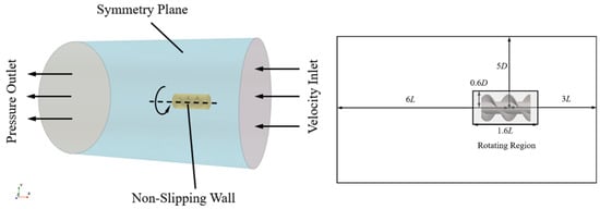
Figure 4.
Calculation domain with the associated boundary conditions.
The inlet boundary was set as a uniform velocity inlet, and the outlet was specified as a constant static pressure outlet. A no-slip wall condition was imposed on the propulsor surface, and the interface between the rotating and stationary domains was handled using a general sliding interface condition. The inlet velocity was set to correspond to advance coefficients J.
3.3. Numerical Method and Model
Both the steady and unsteady simulations employed the Moving Reference Frame (MRF) approach to model the rotation of the screw propulsor. This method treats the rotating region as a steady rotating frame of reference, allowing for simplified mesh treatment and efficient computation of rotating flow without requiring mesh motion. In the unsteady simulations, the MRF was coupled with the DDES turbulence model to resolve transient vortex structures while maintaining computational stability.
The software STAR-CCM+ 2206 (17.04.007-R8) was used in this study to conduct simulations, and all discretization techniques are presented in Table 2. This table outlines the key discretization schemes used for DDES with the SST turbulence model. The pressure–velocity coupling employs a SIMPLE algorithm for unsteady flows, while time integration uses a second-order implicit scheme. Wall treatment follows the low y+ approach for accurate boundary layer resolution. The solver combines pressure-based formulation with DDES turbulence modeling using IDDES coefficients. The transient simulations employed a time step size of 0.0002 s, as it ensures that the propulsor rotates at least 1° in each time step.
Table 2.
Discretization techniques.
3.4. Computational Grid
For the steady-state simulations, trimmed meshes were employed for efficient computation. For the unsteady simulations, the grid’s resolution should meet the requirements of the DDES model to capture the small-scale flow structure mechanisms. Figure 5 displays the generated grids over the calculation domain. All grids were generated with tetrahedral elements. Grid 1 was first established as the base size across the entire calculation domain. Volume controlling was then applied to obtain an intermediate grid (Grid 2), and a refined grid (Grid 3) to resolve the detailed flow structures near the blades and in the wake. A separate rotating grid block (Grid 4) was employed to capture the motion of the screw propulsor, and there is a sliding interface around the rotating domain. Prism layer grids (Grid 5) were generated near the propulsor surface to ensure , allowing accurate resolution of the boundary layer and appropriate transition to turbulence. Correspondingly, Table 3 lists the details of five different grids, where a total of approximately 8.5 million cells were generated. The mesh quality was assessed using mesh diagnostics. Over 90% of the cells in the flow domain had quality function values above 0.9, with skewness mainly ranging between 25° and 35°, and aspect ratios above 0.95. In the rotating region, 90% of cells achieved mesh quality over 0.7, with skewness in the range of 20°~40° and aspect ratios over 0.85. These values indicate that the mesh is suitable for resolving key flow structures with sufficient accuracy.
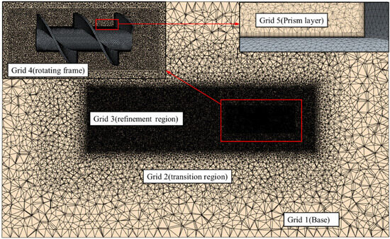
Figure 5.
Generated grids over the calculation domain.
Table 3.
Grid configuration details.
4. Results and Discussion
4.1. Propulsive Performance Under Different Geometric Parameters
In total, 36 steady-state simulations were conducted, covering a two-dimensional design space defined by diameter ratio and helix angle. For each configuration, the maximum propulsive efficiency across the full range of advance coefficients () was extracted for comparison, as shown in Figure 6a.
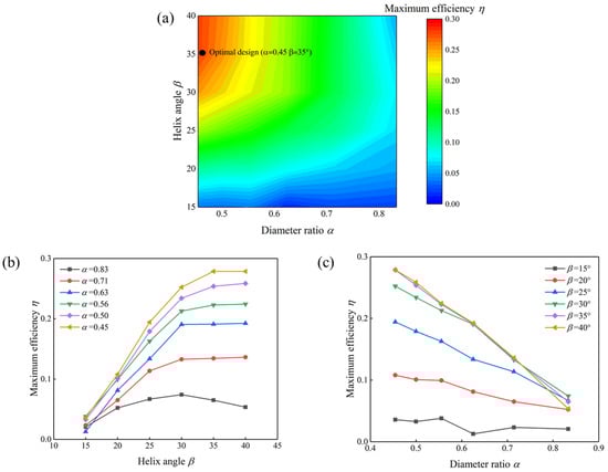
Figure 6.
Influence geometric parameters on propulsive performance. (a) Maximum efficiency distribution in the parameter space with the optimal configuration marked. (b) Maximum efficiency variation with helix angle at different diameter ratios. (c) Maximum efficiency variation with diameter ratio at different helix angles.
Figure 6b revealed that the helix angle had a non-linear effect on propulsive efficiency. A notable improvement in maximum efficiency was observed when the helix angle was increased to 30° or higher. However, further increasing the angle to 40° did not yield significant gains. This suggests a saturation trend beyond 35°, and from a practical manufacturing perspective, larger helix angle can induce severe blade twisting, which may complicate fabrication and increase the challenge to the strength of the blades. Therefore, an angle of 35° was found to yield the highest efficiency.
Figure 6c illustrates that, at a fixed helix angle, reducing the diameter ratio consistently enhanced the efficiency. This implies that increasing blade height contributes positively to thrust production, due to the increased projected area interacting with flow. Interestingly, the efficiency curves did not exhibit a plateau even at the lowest diameter ratio, indicating that there is still space for improvement in blade height within the current design space.
Another important observation is that, at low helix angle, increasing blade height did not significantly improve efficiency. This may be attributed to the reduced helix pitch under small inclinations, which narrows the spacing between adjacent blades and may cause flow interference effects. Based on a comprehensive evaluation, the optimal configuration was identified at and . To further investigate this discrepancy, this configuration was selected for the subsequent transient simulations aimed at exploring the unsteady flow characteristics in detail.
4.2. Transient Flow Field Analysis of the Optimal Configuration
Based on the configuration identified in Section 4.1, transient hydrodynamic simulations were conducted using the DDES model under rotational speeds of 200 rpm, 400 rpm, and 600 rpm. A fixed free stream velocity 0.5 m/s was applied. The following subsections present a detailed analysis of the unsteady flow structures and hydrodynamic characteristics.
4.2.1. Spectral Characteristics and Dominant Frequency
To investigate the unsteady characteristics, time-resolved data of pressure and velocity were collected at six monitoring points under the three rotational speeds. As shown in Figure 7, the first three points are located near the blade tip region, and the last three points are distributed along the downstream axis. At each operating condition, the monitoring signals were processed using Fast Fourier Transform (FFT), and the amplitude spectra were extracted to identify the dominant frequency components [18]. The frequency spectra are presented in Figure 8, Figure 9 and Figure 10. The theoretical blade passing frequency (BPF) could be defined as follows:
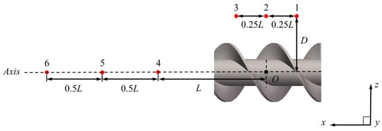
Figure 7.
Monitoring points.
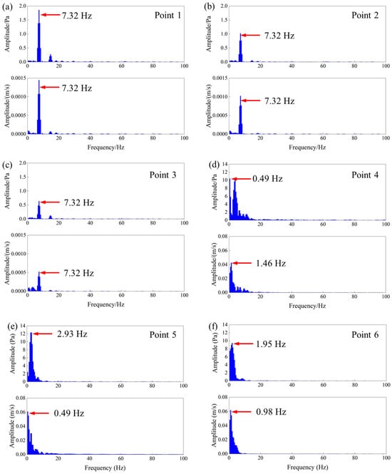
Figure 8.
FFT results of pressure and velocity signals at monitoring points under 200 rpm. (a) Point 1. (b) Point 2. (c) Point 3. (d) Point 4. (e) Point 5. (f) Point 6.
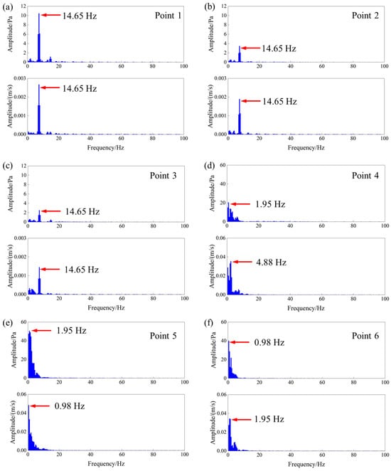
Figure 9.
FFT results of pressure and velocity signals at monitoring points under 400 rpm. (a) Point 1. (b) Point 2. (c) Point 3. (d) Point 4. (e) Point 5. (f) Point 6.
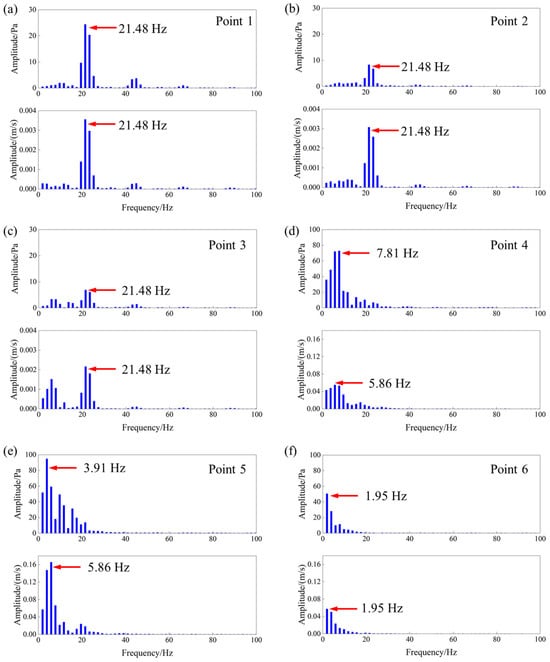
Figure 10.
FFT results of pressure and velocity signals at monitoring points under 600 rpm. (a) Point 1. (b) Point 2. (c) Point 3. (d) Point 4. (e) Point 5. (f) Point 6.
Figure 8 presents the amplitude spectra of the pressure and velocity signals at six monitoring points under 200 rpm rotational speed. For the first three points, both the velocity and pressure signals exhibited a dominant frequency of 7.32 Hz, which is slightly higher than the theoretical BPF of 6.67 Hz at 200 rpm. This consistent dominant frequency reflects the strong periodic nature of the near blade flow induced by the rotation. The dominant frequency dominated the spectra with progressively decreasing amplitudes, and this trend indicates the gradual attenuation of blade-induced periodic disturbances due to viscous dissipation and flow diffusion.
Point 4 exhibited a significant increase in amplitude, despite a shift to a lower dominant frequency. This marks the onset of wake-induced unsteadiness, where large-scale vortex shedding or flow instability replaces the blade-induced periodicity. The amplitude further increased at point 5, suggesting a region of energy reorganization or vortex merging. At point 6, both the amplitude and frequency decreased again, indicating the break-down and dissipation of coherent structures in the far wake.
As shown in Figure 9, the points 1–3 still exhibited strong BPF dominance, with the dominant frequency observed at 14.65 Hz, which is precisely twice the value observed under the 200 rpm condition. This confirms the linear relationship between BPF and rotational speed. The dominant frequency shifted toward lower values at points 4–6, while the spectral amplitudes first increased and then decreased. This consistency suggests that higher rotational speeds elevate the BRF.
At 600 rpm, the dominant frequency at the first three monitoring points near the blade tip was 21.48 Hz, which is approximately three times the dominant frequencies observed at 200 rpm. Additionally, the amplitude decay along the flow direction remains consistent with previous conditions, indicating a general spatial attenuation of the blade-induced disturbance.
Notably, at point 3, a secondary peak emerged with an amplitude nearly equal to that of the dominant frequency. This suggests the presence of secondary flow structures or nonlinear interactions such as vortex-wake interference or shear-layer instabilities, which intensify the energy at higher harmonics and contribute to more complex unsteady flow features at this location.
The FFT analysis of pressure and velocity signals under the three conditions consistently revealed a dominant frequency that scales linearly with the rotational speed. This confirms that the dominant frequency in the near-rotation region can be regarded as the equivalent blade-passing frequency (EBPF), defined as follows:
where is the number of the helix line. The results imply that the dominant frequency stems from the EBPF. The consistent frequency patterns observed at monitoring points near the blade tip confirm the regular periodicity of the blade-induced flow structures. However, the pressure and velocity signals at downstream axial points exhibited differing dominant frequencies.
Based on the identified dominant frequencies, the corresponding characteristics’ time periods were defined and used to extract instantaneous flow field data, and they are approximately 0.137 s, 0.068 s, and 0.047 s.
4.2.2. Flow Field Evolution Based on Dominant Frequency
The BPF identified through FFT analysis was used to determine the period T, which was then used to extract instantaneous flow field data at multiple phase: 0T, 0.25T, 0.5T, 0.75T, and 1T. The analysis focuses on four key flow variables: axial velocity, negative pressure coefficient, turbulent kinetic energy (TKE), and vorticity. These variables could provide complementary insight into flow field characteristics.
To enable consistent comparison of axial velocity distribution under different rotational speed conditions, a dimensionless procedure was applied. Specifically, the axial velocity u was normalized by the blade tip velocity , defined as follows:
Under the operating condition with a rotational speed of 200 rpm, the computation time is 2 s. We selected 1.8 s as the time. Based on the FFT analysis above, the characteristic period T is 0.137 s. Figure 11 presents the axial velocity contours in the longitude section, where the velocity wake remains relatively symmetric and narrow. Around the rotating region, particularly near the blade tip, a distinct pattern of paired high and low-speed local regions is observed in front of each blade and close to the blade. This vertical velocity gradient suggests the presence of a velocity shear layer, possibly associated with blade-induced flow acceleration combined with flow separation effects near the blade. Surrounding the blade tips, the flow field reveals alternating zones of axial acceleration and deceleration, forming quasi-periodic fluctuation of axial velocity.
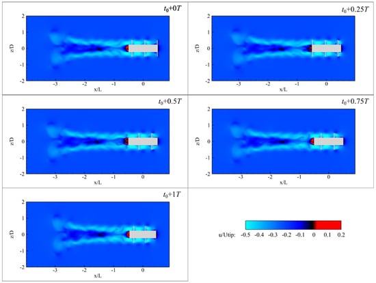
Figure 11.
Axial velocity fields at the typical moments for 200 rpm rotational speed.
In the wake region near the structure’s trailing edge, a reverse flow region develops, suggesting the presence of unsteady boundary layer separation or localized vortex recirculation. During the period, the reverse flow experiences the process of deceleration and reformation. This variability indicates the strong unsteady nature of vortex-induced pressure gradients.
Around the location of , the velocity contours exhibit a pronounced wake contraction, characterized by a narrowing of the axial velocity profile toward the axis. This constricted region results from the interaction between the rotational wake and the surrounding entraining fluid. The narrowing of the wake around this region implies that the central momentum is being compressed and focused.
Further downstream around the location of , a low-speed zone begins to appear, and the axial velocity even approaches zero, indicating the formation of a quasi-stagnant core. The velocity drops significantly, due to momentum diffusion from the upstream contraction. When reaching the downstream location , the velocity starts to recover, and the previously stagnant flow gradually disappears. The overall wake widens slightly.
The distribution of the negative pressure coefficient defined [19] as follows:
it is employed to highlight low-pressure zones that are critical in understanding vortex formation and energy conversion efficiency. Here, p is the static pressure at the point of the interest, is the free-stream pressure, and is the fluid density. As shown in Figure 12, the negative pressure coefficient distribution generally follows the expected trend for a rotating structure in axial flow. A localized high-suction region appears near the leading edge of each blade, while a corresponding blue region of relatively higher pressure is found on the pressure side.
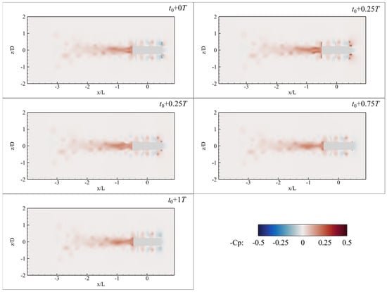
Figure 12.
Contour of the pressure coefficient at the typical moments for 200 rpm rotational speed.
In the wake, a continuous zone of relatively high negative pressure extends from the propulsor trailing edge to approximately along the axis; then, the negative pressure gradually diminishes. This suggests the occurrence of a wake contraction phenomenon.
As shown in Figure 13, the TKE remains relatively low across the domain at 200 rpm. The elevated TKE zones are primarily localized near the propulsor surfaces and the immediate vicinity of the propulsor trail, reflecting weak turbulence generation and relatively stable flow separation.
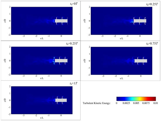
Figure 13.
Contour of the TKE at the typical moments for 200 rpm rotational speed.
The vorticity magnitude, serving as a key indicator of local rotational intensity in the flow field, helps identify shear layers, vortex structures, and regions of flow separation. As shown in Figure 14, the vorticity is predominantly concentrated in the downstream region of the propulsor, indicating most of the energy dissipation and vortex generation occurs in the wake. Within the rotating region, circular zones of high vorticity are observed on the upstream sides of the blades, corresponding to the formation of vortex cores near the blade surfaces due to strong shear effects.
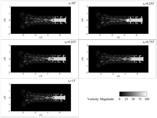
Figure 14.
Contour of the vorticity magnitude at the typical moments for 200 rpm rotational speed.
In the wake region, the vorticity field exhibits banded or arc-shaped high-vorticity zones. These structures originate from shear layers formed at the separation points where the flow detaches from the blade surfaces. As the separated shear layers evolve downstream, they roll up into vortices due to Kelvin–Helmholtz instability, giving rise to coherent vortex structures that are advected with the main flow. These features highlight the important role of wake instabilities in the flow dynamics.
Under the operating condition with a rotational speed of 400 rpm, the computation time is 1.5 s, and we have chosen 1.4 s as the time. Based on the FFT analysis, T is 0.068 s. Figure 15 presents the axial velocity contours at a rotational speed of 400 rpm, and the axial velocity exhibits intensified flow features compared to the 200 rpm condition. The high-speed zones near the blade tips become more pronounced and shift slightly away from the blade surface, indicating stronger centrifugal effects and blade-induced acceleration. However, the associated low-speed zones are now noticeably smaller in spatial extent, though their minimum velocities further decrease, approaching stagnant levels. The low-speed zones closer to the front of the propulsor structure are more pronounced.
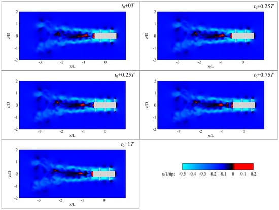
Figure 15.
Axial velocity fields at the typical moments for 400 rpm rotational speed.
In the wake region, the flow exhibits a continued narrowing of the velocity core near the trailing edge. However, this contraction phenomenon becomes less distinct, with the narrowing initiating upstream of and transitioning into a velocity stagnation zone immediately downstream. A reverse flow emerges near . As the flow continues downstream, the reverse flow gradually decreases and a stagnation zone appears. The stagnation zone persists downstream and extends to approximately , indicating a longer-range influence on the surrounding fluid. The presence of such a reversed flow structure indicates enhanced flow separation and energy loss.
As shown in Figure 16, the low-pressure regions remain prominent on the pressure side of the leading blades, but gradually shift toward the tips in the downstream blades. Between the trailing edge and , the pressure coefficient remains significantly negative, indicating the presence of a low-pressure zone. Further downstream, in the region from to , the pressure near the axis becomes less negative, while a series of isolated circular zones with highly negative pressure appear symmetrically along the outer edge of the wake. These structures coincide with the locations of strong velocity gradients and recirculation zones, indicating the localized flow separations of shear-induced vortices near the periphery of the wake.
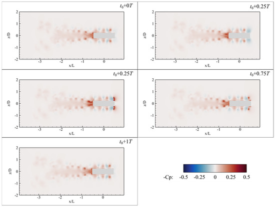
Figure 16.
Contour of the pressure coefficient at the typical moments for 400 rpm rotational speed.
As shown in Figure 17, TKE becomes more pronounced at 400 rpm. In particular, the region extending from the trailing edge to approximately shows intensified turbulent activity. This corresponds to the onset of more prominent wake stabilities and vortex interactions. Around the rotating blades, the TKE also increases, especially near the tip, where high velocity gradients enhance local turbulence production.
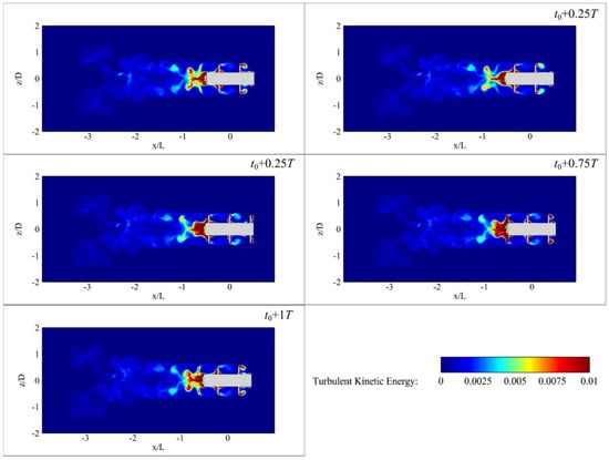
Figure 17.
Contour of the TKE at the typical moments for 400 rpm rotational speed.
As shown in Figure 18, the vorticity field becomes considerably more structured at a rotational speed of 400 rpm. Within the rotating region, vortex cores become more pronounced and intense. Downstream of the propulsor, from the trailing edge to approximately , a broad region of elevated vorticity is observed. This zone is associated with the generation of coherent vortices. Further downstream ( to ), a series of discrete vortex cores emerges. These vortices exhibit a nearly axisymmetric pattern with relatively regular spacing, indicating a developing vortex street. Their formation is attributed to the periodic breakdown of upstream shear-layer vortices, as well as continuous perturbations imposed by the rotating flow. This periodic shedding behavior corresponds with the unsteady features previously observed in the velocity and pressure coefficient contours. The high-vorticity region extends from the surface of the propulsor to a much farther wake region, indicating stronger vortex generation and transport.
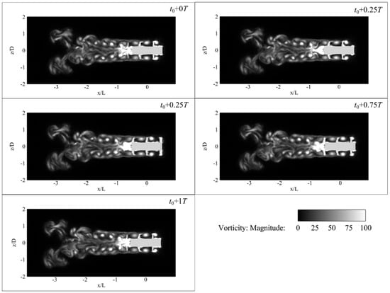
Figure 18.
Contour of the vorticity magnitude at the typical moments for 400 rpm rotational speed.
The computation for 600 rpm operating condition is 1 s. We have chosen 0.9 s as the time. Based on the FFT analysis, T is 0.047 s. As shown in Figure 19, within the rotating region, the inter-blade spaces are almost entirely occupied by high-speed zones, which have expanded noticeably compared to lower rotational speeds. This indicates an enhanced acceleration effect exerted by the screw propulsor. The associated low-speed zones also expand slightly. Notably, distinct reverse flow bubbles appear within the low-speed zone at the front. This phenomenon is induced by strong centrifugal effects near the blade tips coupled with adverse pressure gradients that promote local flow separation and vortex roll-up. The formation of such reverse flow structures indicates a higher degree of unsteadiness and potential vortex core development in this high-speed regime.
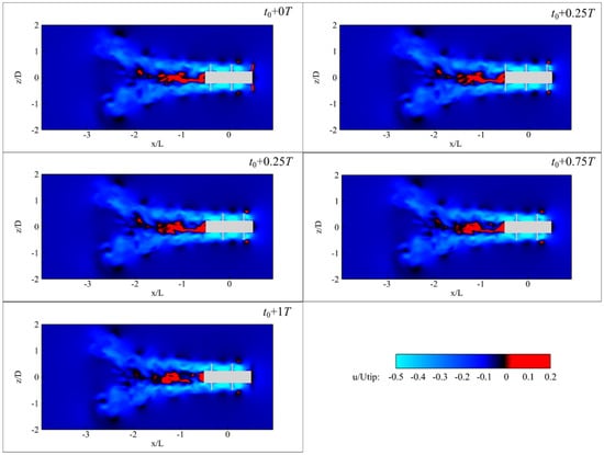
Figure 19.
Axial velocity fields at the typical moments for 600 rpm rotational speed.
In the wake region, the flow no longer shows the pronounced contraction. Instead, a significant asymmetric reverse flow region emerges near the trailing edge of the propulsor and extends downstream up to , which reflects a highly disturbed wake structure dominated by non-periodic behaviors and enhanced turbulence. Furthermore, the paired high–low speed zones, initially observed in the rotating region, persist into the downstream wake and remain observable along the outer boundary of the wake. This indicates that the shear-induced vortex structures generated by the rotating motion can maintain coherence over a long distance. The increased prominence of these structures at 600 rpm is attributed to very low axial velocity in the wake periphery, leading to sharper gradients and more distinct velocity contrasts.
As shown in Figure 20, the distribution of the pressure coefficient within the rotating region remains consistent with the 400 rpm condition. In the wake region, a distinct high-pressure zone is still observed near the propulsor trailing edge. However, beginning from approximately , the negative gradually weakens along the axis, indicating a weakening of flow contraction. This trend corresponds well with the axial velocity fields, where wake narrowing becomes minimal at this operating condition.
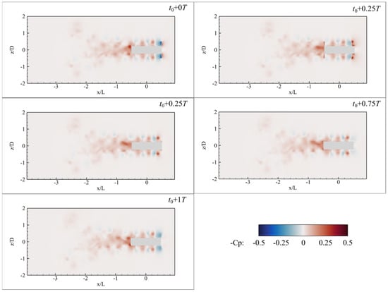
Figure 20.
Contour of the pressure coefficient at the typical moments for 600 rpm rotational speed.
Another distinct feature is the appearance of red and blue patches along the wake periphery. This pattern reflects periodic vortex shedding or interactions within the wake shear layer. Overall, the limited extent of high negative pressure zones, the weakening of wake contraction, and the emergence of symmetric pressure pairs suggest that, under higher rotational speeds, the wake becomes more spread out and the low-pressure regions less concentrated, even though the wake still retains certain periodic structures.
As shown in Figure 21, the flow field exhibits the most complex and energetic turbulent structures at 600 rpm. High TKE zones expand downstream, covering the entire region from the tail edge to beyond . Additionally, the blade wake regions become more turbulent, with elevated TKE not only confined to the tip regions, where high velocity gradients enhance local turbulence production.
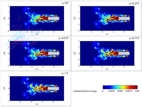
Figure 21.
Contour of the TKE at the typical moments for 600 rpm rotational speed.
As shown in Figure 22, the vorticity distribution becomes significantly more intense and structurally complex compared to lower rotational speeds. Within the rotating region, brighter circular patches of high vorticity are observed. There regions represent enlarged primary vortex cores, whose size and intensity are enhanced due to the stronger centrifugal effects and shear associated with increased rotational speed.
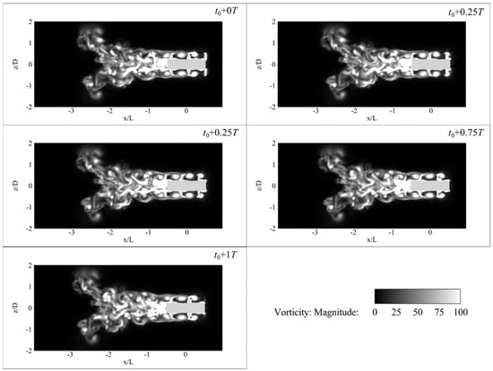
Figure 22.
Contour of the vorticity magnitude at the typical moments for 600 rpm rotational speed.
In the near wake region downstream of the propulsor trailing edge (up to ), a band of elevated vorticity forms, consistent with the development of shear-layer vortices resulting from flow separation. However, unlike the 400 rpm case where a series of symmetric, regularly spaced vortex cores extend from to , the 600 rpm condition shows no such periodic structure. Instead, irregular, and asymmetric, high-vorticity zones appear in this region, resulting from the break-down of initial coherent vortices and the generation of secondary vortices due to turbulent instabilities.
Moreover, while the local vorticity intensity is higher, the wake’s spatial influence appears more confined, with prominent structures dissipation before reaching . This reduced extent of the wake, despite the higher input energy, may be attributed to intensified turbulent dissipation at higher rotational speeds. The disintegration of organized vortex structures prevents sustained downstream transport of vorticity. The transition from organized to chaotic vorticity patterns in the far wake reflects a regime where turbulent diffusion dominates over convective persistence.
Therefore, this suggests that, while higher rotational speeds enhance local vorticity generation, they also accelerate the break-down and dissipation of wake structures, resulting in a shorter yet more turbulent wake field.
In summary, the detailed flow field analysis across varying rotational speeds reveals several hydrodynamic characteristics unique to the screw propulsor. The velocity contours demonstrate that thrust is primarily generated by the axial acceleration of fluid within the rotating domain. Distinct high and low-speed regions emerge periodically around the blades, particularly forming paired structures along the blade gaps. These structures become more prominent and complex with increasing rotational speed, indicating intensified blade-induced flow and shear.
In the wake region, the pressure and vorticity fields jointly illustrate a multistage flow evolution process. Initially, strong low-pressure zones and shear layers are formed downstream of the blade trailing edge, accompanied by periodic shedding of coherent vortex structures. These vortex cores, particularly clear under moderate rotational speeds, exhibit a symmetric distribution and contribute to axial momentum transfer. However, at a higher rotational speed, these coherent structures tend to disintegrate rapidly, leading to a more chaotic and dissipative flow regime. The breakdown of organized vortices, driven by shear-layer instabilities and Kelvin–Helmholtz mechanisms, marks the transition from ordered propulsion to turbulent diffusion.
This unsteady evolution of vortical structures underscores the propulsion mechanism of the propulsor, where the rotating blades continuously impart energy to the surrounding fluid, forming vortex rings and jet-like axial acceleration zones that push water rearward, thereby generating forward thrust. However, much of the injected energy is not retained in coherent structures but instead dissipated through turbulent mixing and vortex break-down. The high levels of turbulent kinetic energy and widespread vorticity downstream indicate that energy loss through viscous dissipation is substantial. Compared to traditional propellers, which maintain more stable tip vortices and streamlined axial jets, the screw propulsor suffers from rapid energy dispersion and less efficient conversion of rotational input into directed momentum. The presence of disordered wake structures and high turbulent losses partially explains the relatively lower propulsion efficiency of this configuration. Its complex hydrodynamic characteristic emphasizes the tradeoff between compact design and energy efficiency.
To further understand the spatial organization and three-dimensional dynamics of these vortical structures, the visualization and analysis of the vortex topology are presented in the next section. This will offer deeper insights into the unsteady mechanisms governing wake evolution and energy dissipation.
4.2.3. Vortex Structure Evolution and Dynamics
To further reveal the unsteady hydrodynamic characteristics induced by the screw propulsor, this section will investigate the three-dimensional vortex structures. The vortex structures are extracted based on the Q-criterion, which identifies rotationally dominated regions where the magnitude of the vorticity tensor exceeds that of the strain rate tensor. In this study, iso-surfaces corresponding to s−2 are selected to visualize coherent vortex structures.
Initially, the evolution process is visualized through Q-criterion iso-surfaces colored by vorticity magnitude, covering multiple time phases: 0T, 0.25T, 0.5T, 0.75T, 1T, 1.25T, and 1.5T. These images highlight the dynamic formation, shedding, and dissipation of vortex cores. Subsequently, snapshots corresponding to the same phase were selected for the three conditions. These vortex structures were visualized with scalar field coloring based on non-dimensional axial velocity and negative pressure coefficient, and the mappings provide complementary insight into momentum transport and pressure gradients associated with vortex evolution.
In the near wall rotational region, tip vortices are generated at the blade tips due to strong shear effects during blade rotation. Owing to the continuous helix structure of the blades, which are periodically distributed in space, the evolution of tip vortices is significantly influenced by the periodic reappearance of the blade downstream part. Once formed upstream, the tip vortices detach from the blades and are transmitted downstream under the influence of the mainstream flow and their own inertia. When transported through the gaps between blades, the vortices can move relatively unobstructed. However, upon encountering subsequent downstream blades, they experience interruption, deformation, or partial dissipation due to the additional shear and obstruction. These interactions may lead to vortex tearing, deflection, or partial energy absorption by the blades. This phenomenon is shown in Figure 23, which presents the progressive reduction in vortex tube diameter and even the disappearance of the vortex structures.
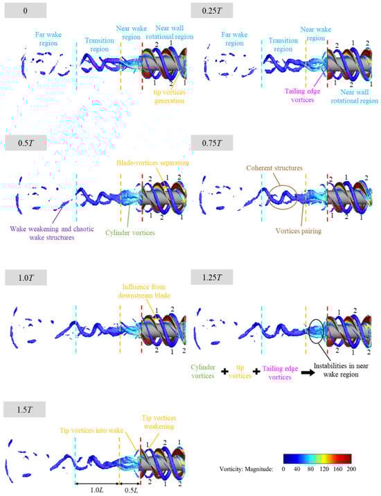
Figure 23.
Vortex structure evolution at 200 rpm visualized by Q-criterion iso-surfaces ( s−2) colored by vorticity magnitude. The initial time 0T corresponds to 1.8 s, consistent with Section 4. Numerical labels ‘1’ and ‘2’ mark the tip vortices tubes generated by the two blades. The red dashed line denotes the trailing edge of the propulsor, while the yellow and blue lines mark the axial locations and .
In the near wake region, tip vortices, trailing edge vortices, and cylinder vortices shed from the rotating blades interact and merge near the propulsor trail. This convergence results in multi-vortex interference, including vortex pairing, shear layer interaction, and vortex tearing, leading to an unsteady and highly disordered near-wake flow. In the transition region, around the location marked by the yellow line, vortex pairing occurs once again, producing larger coherent vortex structures. These reorganize into a tilted but relatively ordered helical vortex street, which can be regarded as a coherent vortex transition region. Further downstream, in the far wake region, the vortices continue to stretch and break apart, and their energy is gradually dissipated. Eventually, the flow transitions into a fully turbulent state, marking the complete breakdown of organized vortex structures.
Under the 400 rpm condition, vortex transport extends further downstream, accompanied by enhanced momentum diffusion and intensified small-scale turbulence after vortex breakdown, which promotes lateral mixing and wake broadening, as shown in Figure 24.
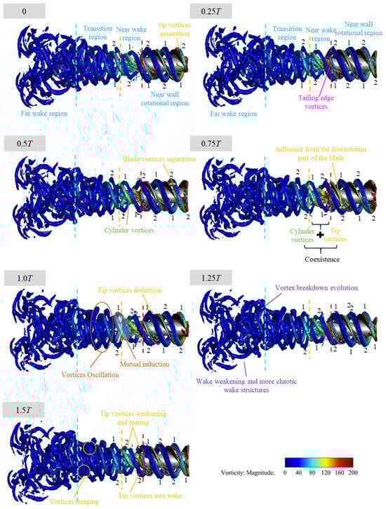
Figure 24.
Vortex structure evolution at 400 rpm visualized by Q-criterion iso-surfaces ( s−2) colored by vorticity magnitude. The initial time 0T corresponds to 1.4 s, consistent with Section 4. Numerical labels ‘1’ and ‘2’ mark the tip vortices tubes generated by the two blades. The red dashed line denotes the trailing edge of the propulsor, while the yellow and blue lines mark the axial locations and .
In the near wall rotational region, the increase in rotational speed enhances both the strength and size of the vortex tubes. The kinetic energy and circulation of the tip vortices are elevated, allowing them to resist interference from downstream blades and maintain structural integrity during downstream transport. In the near wake region, intensified rotation induces strong cylinder vortices, forming a more coherent vortex street. Tip vortices and cylinder vortices coexist and interact, with centrifugal effects causing radial expansion. As the cylinder vortices spirals widen, mutual induction effects between the tip and cylinder vortices emerge, leading to changes in vortex spacing and localized deformation of vortex cores.
In the transition region, the reduced spacing between vortex tubes results in stronger induced velocities. Mutual interactions between vortices lead to positional oscillations, gradually triggering instabilities. Consequently, the initially orderly spiral vortex tubes become distorted and entangled. In the far wake region, vortex merging occurs, where smaller vortices combine into larger structures. With continued downstream transport, the vortex tubes eventually fall apart and break down into turbulent patches.
At 600 rpm, shown as Figure 25, the wake exhibits no distinct transition region. The flow becomes disordered immediately downstream of the near wake region, and vortex breakdown initiates near the yellow line. In the near the wake region, the previously clear periodicity of the cylinder vortices disappears. The cylinder vortices merge with the tip vortices, resulting in blurred boundaries and indistinct individual structures. These large vortices rapidly transition into turbulence, indicating strong vortex breakdown. Due to intensified energy dissipation and centrifugal effects, the wake becomes short and wide. Axial momentum is dispersed by rotational effects, weakening the axial transport capability of the flow. This reflects a reduction in coherent vortex structures and a more chaotic flow regime in the far wake region.
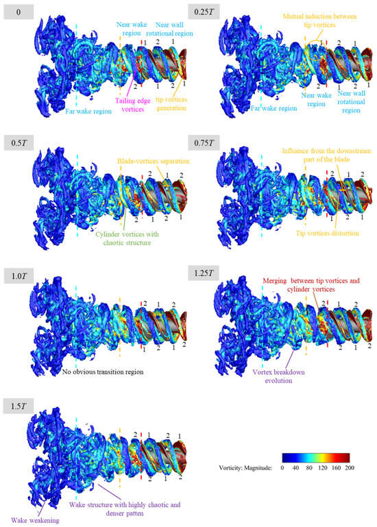
Figure 25.
Vortex structure evolution at 600 rpm visualized by Q-criterion iso-surfaces ( s−2) colored by vorticity magnitude. The initial time 0T corresponds to 0.9 s, consistent with Section 4. Numerical labels ‘1’ and ‘2’ mark the tip vortices tubes generated by the two blades. The red dashed line denotes the trailing edge of the propulsor, while the yellow and blue lines mark the axial locations and .
Figure 26 clearly reveals the transition from an ordered vortex street at low rotational speeds to a fully turbulent wake at high speeds. This evolution fundamentally reflects the competition among inertial, centrifugal, and viscous forces within the rotating flow. At 200 rpm, the wake remains relatively coherent, with weak reverse flow occasionally observed, yet the flow is predominantly governed by the axial mainstream. The vortex shedding frequency is low, and energy dissipation occurs slowly. At 400 rpm, alternating regions of high and low axial velocity appear in the wake, suggesting enhanced vortex–vortex interactions and the emergence of induced velocities between neighboring vortices. The rotational effect becomes more pronounced, and eddy kinetic energy plays a more dominant role in shaping the wake evolution. At 600 rpm, the wake displays clear features of strong turbulence. Vortex cores become unstable and break apart due to centrifugal instabilities, resulting in a more disordered vortex field. In this regime, vortex break-down becomes the primary mechanism of energy dissipation, marking the transition to turbulence dominated by nonlinear interactions and turbulent diffusion.
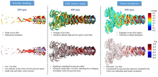
Figure 26.
Vortex structures of the propulsor at 200 rpm, 400 rpm, and 600 rpm under the same phase, colored by nondimensional axial velocity (top row) and negative pressure coefficient (bottom row).
4.3. Uncertainty Discussion
Although direct experimental validation was not conducted due to the scarcity of available reference data and current limitations in experimental infrastructure, several measures were adopted to ensure the reliability of the numerical results. The simulations employed a sufficiently refined mesh characterized by favorable quality metrics, with over 90% of cells exhibiting skewness angles below 35°, and aspect ratios consistently exceeding 0.95 across most computational regions. A second-order implicit temporal discretization scheme was utilized to minimize numerical dissipation and improve solution accuracy.
Furthermore, the periodicity of the unsteady flow was rigorously identified using time-series data from internal monitoring points. The evolution of flow structures, such as vortices and pressure fields, was consistently observed to follow physically reasonable and repeatable trends across multiple rotational speeds. These observations collectively enhance the credibility of the results by supporting internal physical consistency.
While quantitative uncertainty analysis was not performed, uncertainties due to numerical settings are estimated to be within an acceptable range, with deviations unlikely to exceed 5% for capturing key flow mechanisms. Future validation, including planned Particle Image Velocimetry (PIV) experiments, will help further evaluate and refine the numerical accuracy of the present findings.
5. Conclusions
Our work presents a comprehensive flow field analysis of a screw propulsor, offering detailed insights into its propulsion mechanism across different rotational speeds. The results demonstrate the following:
(1) Thrust generation primarily arises from the interaction between blade-induced tip vortices, cylindrical body vortices, and trailing-edge shedding vortices.
(2) As the rotational speed increases, the wake evolves from an orderly vortex street into a chaotic turbulent region, primarily driven by centrifugal and inertial instabilities.
(3) Key flow phenomena—including vortex pairing, elongation, reconnection, and breakdown—dominate the downstream dynamics, especially within transitional and far-wake regions.
(4) These complex vortex dynamics result in enhanced radial momentum diffusion and premature vortex breakdown, which together disrupt axial momentum delivery and diminish propulsion effectiveness.
These characteristics collectively result in a propulsion process that is highly dynamic yet inefficient. Compared to traditional propellers, the screw propulsor exhibits greater radial energy dispersion and earlier vortex collapse, weakening axial thrust and increasing viscous losses. These insights suggest that future design improvements may focus on controlling vortex development and mitigating radial energy dispersion, such as by optimizing blade geometry, introducing guide vanes, or incorporating flow control strategies to enhance axial momentum preservation and reduce unsteady losses.
Author Contributions
Y.K.: Writing—original draft, Methodology, Formal analysis, Investigation. P.X.: Conceptualization, Project administration, Funding acquisition. M.C.: Formal analysis, Investigation, Writing—review. L.Y.: Resources. All authors have read and agreed to the published version of the manuscript.
Funding
This research was funded by National Key Research and Development Program of China grant number 2022YFC2806002 and 2021YFC2801604, National Natural Science Foundation of China grant number 52071131 and Frontier Technologies R&D Program of Jiangsu Province grant number BF2024072.
Data Availability Statement
The original contributions presented in this study are included in the article. Further inquiries can be directed to the corresponding author.
Acknowledgments
The authors sincerely appreciate the valuable comments and constructive suggestions from the editors and reviewers, which have significantly improved the quality and structure of this manuscript.
Conflicts of Interest
The authors declare that they have no conflicts of interest to disclose.
References
- Villacrés, J.; Barczyk, M.; Lipsett, M. Literature review on Archimedean screw propulsion for off-road vehicles. J. Terramechanics 2023, 108, 47–57. [Google Scholar] [CrossRef]
- Welling, C.G. An Advanced Design Deep Sea Mining System. In Proceedings of the Offshore Technology Conference, Houston, TX, USA, 4 May 1981. [Google Scholar] [CrossRef]
- ROBOMINERS. Available online: https://robominers.eu/ (accessed on 24 May 2024).
- Helix Robots Capabilities. Available online: https://copperstonetech.com/ (accessed on 1 February 2025).
- Sandakov, M.Y.; Mukhina, M.L.; Shurina, A.A.; Krasheninnikov, M.S.; Dorofeev, R.A. The Study of Seaworthiness of Universal Rescue Vehicle with Rotary Screw Propeller. In Proceedings of the 2015 International Conference on Advanced Manufacturing and Industrial Application; Atlantis Press: Phuket, Thailand, 2015. [Google Scholar] [CrossRef][Green Version]
- Karaseva, S.; Papunin, A.; Belyakov, V.; Makarov, V.; Malahov, D. Structural Analysis of Hydrodynamical Interaction of Full-Submerged Archimedes Screws of Rotary-Screw Propulsion Units of Snow and Swamp-Going Amphibious Vehicles with Water Area via Methods of Computer Simulation. Eng. Proc. 2023, 33, 32. [Google Scholar] [CrossRef]
- Xu, P.F.; Lin, H.L.; Kai, Y.; Su, J.Y.; Hu, Q. Research on Screw Propulsion Performance of Amphibious Robot. J. Unmannned Undersea Syst. 2024, 32, 1063–1071. [Google Scholar] [CrossRef]
- Bishop, R.; Wright, J.; Beknalkar, S.; Juarez-Vera, R.; Yount, K.; Stimach, M.; Basuroski, A.; Bryant, M.; Mazzoleni, A. Design, Prototyping, and Experimentation of a Dual Helical Drive Vehicle for Underwater Exploration. In Proceedings of the OCEANS 2024—Halifax, Halifax, NS, Canada, 23–26 September 2024; pp. 1–7. [Google Scholar] [CrossRef]
- Zhu, P.; Dang, P.; Yang, S.; Wu, D. Numerical analysis of propulsion performance of the Archimedean screw under mooring conditions. Proc. Inst. Mech. Eng. Part M J. Eng. Marit. Environ. 2025. online first. [Google Scholar] [CrossRef]
- Donohue, B.; Beknalkar, S.; Bishop, R.; Bryant, M.; Mazzoleni, A. Modeling Underwater Propulsion of a Helical Drive Using Computational Fluid Dynamics for an Amphibious Rover. In Proceedings of the ASME 2023 International Mechanical Engineering Congress and Exposition, New Orleans, LA, USA, 29 October–2 November 2023. [Google Scholar] [CrossRef]
- Ji, B.; Luo, X.; Peng, X.; Wu, Y.; Xu, H. Numerical analysis of cavitation evolution and excited pressure fluctuation around a propeller in non-uniform wake. Int. J. Multiph. Flow 2012, 43, 13–21. [Google Scholar] [CrossRef]
- Pendar, M.R.; Oshkai, P. High-fidelity modeling of cavitating flow around a marine propeller with bio-inspired wavy rudder configurations: Radiated noise analysis using hydro-acoustic analogies. Phys. Fluids 2025, 37, 033375. [Google Scholar] [CrossRef]
- Zhang, Z.; Sun, P.; Pan, L.; Zhao, T. On the propeller wake evolution using large eddy simulations and physics-informed space-time decomposition. Brodogradnja 2024, 75, 75102. [Google Scholar] [CrossRef]
- Lu, S.; Van Hoydonck, W.; Lopez Castaño, S.; Lataire, E.; Delefortrie, G. Numerical study on propeller flow field in four quadrants. Appl. Ocean Res. 2025, 158, 104576. [Google Scholar] [CrossRef]
- Król, P.; Tesch, K. Experimental and Numerical Validation of the Improved Vortex Method Applied to CP745 Marine Propeller Model. Pol. Marit. Res. 2018, 25, 57–65. [Google Scholar] [CrossRef]
- Tian, X.; Ge, H.; Pan, H.; Lv, M.; Zhu, Z.; Xu, H.; Leng, J.; Wang, C. Study on the hydrodynamic characteristics of an outboard engine propeller with hydrophobic coating. Ocean Eng. 2025, 324, 120694. [Google Scholar] [CrossRef]
- Deng, L.; Long, Y.; Ji, B. Delayed detached eddy simulation and vorticity analysis of cavitating flow around a marine propeller behind the hull. Ocean Eng. 2022, 264, 112442. [Google Scholar] [CrossRef]
- He, D.; Wan, D.; Yu, X. Numerical Investigations of Open-water Performance of Contra-Rotating Propellers. In Proceedings of the ISOPE International Ocean and Polar Engineering Conference 2017, San Francisco, CA, USA, 25–30 June 2017. [Google Scholar]
- Posa, A.; Broglia, R.; Balaras, E. The dynamics of the tip and hub vortices shed by a propeller: Eulerian and Lagrangian approaches. Comput. Fluids 2022, 236, 105313. [Google Scholar] [CrossRef]
Disclaimer/Publisher’s Note: The statements, opinions and data contained in all publications are solely those of the individual author(s) and contributor(s) and not of MDPI and/or the editor(s). MDPI and/or the editor(s) disclaim responsibility for any injury to people or property resulting from any ideas, methods, instructions or products referred to in the content. |
© 2025 by the authors. Licensee MDPI, Basel, Switzerland. This article is an open access article distributed under the terms and conditions of the Creative Commons Attribution (CC BY) license (https://creativecommons.org/licenses/by/4.0/).