Comparative Analysis of Recurrent vs. Temporal Convolutional Autoencoders for Detecting Container Impacts During Quay Crane Handling

Abstract

This research develops and validates a novel impact detection system for container monitoring using autoencoders embedded within an edge computing unit. This solution addresses common limitations in current container tracking systems, such as a lack of real-time processing and reliance on cloud connectivity, by enabling local, on-device anomaly detection. We compare the performance of Recurrent Autoencoders (RAEs) and Temporal Convolutional Autoencoders (TCAEs) using acceleration data collected during quay crane handling. Experimental results show that the RAE framework outperforms TCAEs, achieving a precision of 91.3%, a recall of 87.6%, and an F1-score of 89.4% for impact detection while also demonstrating lower reconstruction loss and improved detection of sequential anomalies. The system accurately identifies impact events with minimal computational overhead, proving its viability for real-time deployment in port environments. Our findings suggest that time-series autoencoder architectures, particularly RAEs, are effective for detecting mechanical impacts in resource-constrained edge devices, offering a robust alternative to traditional cloud-based solutions.

1. Introduction

In the recent literature, autoencoder technology has been adopted extensively, ranging from medical data analytics [1] to solving the complex problems of outlier detection [2], from sensory data helping engineers and industry representatives in security process safety applications to helping cybersecurity specialists develop new cybersecurity standards and specialised IoT systems [3]. The already-adopted encoding–decoding techniques are consistently outperformed by newer methods in terms of computational speed and versatility, which has led to their increasing popularity among top-tier researchers across all scientific fields [4,5]. In our previous work [6], we demonstrated the adaptability and efficiency of this approach in detecting specific security events related to shipping containers by analysing acceleration data from sensors mounted on the mechanisms of quay cranes. We have not only demonstrated the exact nature of the problem but also shown that these techniques can be applied in small-scale, embedded edge applications with a security system compatible with other decision support means, detecting even the less visible impacts on the structural integrity of the containers [7,8]. In this paper, we continue our investigation, demonstrating that newer concepts, such as those presented in [9,10], can enhance the adaptability of this technology in the transportation sector as well as among logistics representatives searching for better and more reliable solutions for shock detection, which is currently limited by the computational capabilities of most devices.

Overall, the adoption of novel techniques for damage detection and fault diagnosis in physical systems has been demonstrated by numerous research groups in the engineering field [11,12]. In many cases, autoencoders are generally used to predict specific patterns. In contrast, Lv et al. [13] addressed the problem of link prediction in dynamic (temporal) networks using temporal link prediction approaches, specifically non-negative matrix factorisation (NMF). As a result, they proposed two new deep autoencoder-like NMF models with graph-regularised prediction methods for dynamic networks. Sarikaya et al. [14] analysed machine learning-based intrusion detection systems (IDSs) by estimating the accuracy of their classification results. The authors developed a method that employs generative adversarial networks to produce adversarial attack data and propose a novel RAIDS solution—a robust IDS model designed to be resilient against adversarial attacks in general, utilising the autoencoder’s reconstruction error technique as a prediction value for the classifiers within the estimation metrics. Such direct applications suggest that autoencoders can be used as efficient, supportive tools in combination with more complex techniques [15,16,17,18]. Yet, each case study is unique when higher-order data sets are examined [19,20], which is the primary issue when simplified solutions are applied in large-scale applications, as no unified solution exists [21]. No unified neural network structure exists for the encoder and decoder that can be adopted without any serious modifications [22,23]. Encoder input datasets require refinement, cleaning, and structuring for each specific application [24,25]. Even if similar conditions occur, the same application in different work environments can yield inadequate results [26,27]. This was also highlighted by Danti and Innocenti [28], which strongly supports our claim. They examined this problem and proposed a quality procedure to determine the optimal training set size to minimise the reconstruction error of an autoencoder with predefined structures and hyperparameters that will be trained to encode the expected behaviour of a complex energy generation system.

The application of autoencoders has yet to reach its full potential in direct physical systems and industrial applications due to the complexity of anomaly detection methods [18]. Most existing anomaly detection methods rely not only on training on normal data but also ignore the multi-cluster nature of normal and abnormal patterns. This problem was generally discussed by Zhu et al. [29], who proposed a novel method called the Adaptive Aggregation–Distillation Autoencoder (AADAE) for unsupervised anomaly detection, built upon the density-based landmark selection concerning representing diverse standard patterns. In general terms, anomaly detection among datasets is a vast research field. Autoencoders could indeed improve the situation if adopted in combination with more complex computational techniques, which has been proven by Yan et al. [30], Zhang et al. [31], and Fernandez-Rodriguez et al. [32], as well as incorporating deep learning models within the encoder/decoder [15,33,34] dealing with unsupervised learning problems [35,36,37,38,39,40,41,42,43].

The significance of this paper lies in its intention to fill a gap in the current understanding of how embedded machine learning systems, particularly autoencoders, can be utilised within edge devices to enhance the efficiency and effectiveness of container tracking and monitoring systems. The idea of using an AE in edge devices is relatively fresh, even though NN structures have been utilised for decades. Many authors have already demonstrated their direct applicability in real-life applications. For instance, Zhai et al. [44] proposed an optimisation framework to reduce operational costs in hybrid cloud–edge systems by accounting for mobile user-induced service migration. It introduces the AMGG algorithm, which uses autoencoders and evolutionary techniques to solve complex scheduling problems efficiently. Meanwhile, Yu et al. [45] approached the edge computing challenge from a different angle by presenting a complete three-layer IoT architecture for predictive maintenance, integrating edge, cloud, and application layers to enhance real-time processing and scalability. They introduced a distributed edge-assisted autoencoder to improve performance and efficiency, validated through an industrial case study. Similarly, Goyal et al. [46] proposed a low-cost edge–IoT model using Raspberry Pi 4 and a lightweight LSTM-based autoencoder to detect environmental anomalies in poultry farms. The model achieves real-time inference with an F1-score of 0.9627, enabling accurate and efficient on-device analysis in rural settings, which correlates strongly with the findings presented in our research.

Overall, moving data processing to the edge aims to mitigate common issues such as network congestion and packet loss, thereby improving the reliability and timeliness of critical monitoring tasks [47,48,49]. The outcomes of this research are expected to have significant implications for the design of future logistical monitoring systems that lack stronger innovations. They could lead to the broader adoption of machine learning and edge computing technologies in the logistics industry.

The primary contribution of this research is noteworthy:

• This paper is believed to be one of the first to embed autoencoders in edge sensors for the dynamic condition monitoring of containers. This approach utilises time-series analytics for anomaly detection, showcasing a novel application in the logistics sector.

We propose a novel integration of Recurrent and Temporal Convolutional Autoencoders (RAEs and TCAEs) within an edge computing unit for detecting physical impacts on shipping containers, which has not currently been implemented by any industry representative. While autoencoders have been used in various anomaly detection applications, their deployment in quay crane operations to detect impact-induced anomalies remains unexplored. Our study contributes to this field by demonstrating how time-series autoencoder architectures can effectively capture mechanical impact patterns while operating on resource-constrained edge devices, significantly reducing network reliance and enhancing real-time detection capabilities. Therefore, the objectives of this paper were the following:

• To further test the embedded anomaly detection system by implementing an autoencoder-based anomaly detection system within the selected sensor device. This system will process data locally, reducing the dependency on remote cloud services and minimising the latency and network strain typically associated with large-scale data transmission.
• To validate the system in a live operational environment by testing the robustness and reliability of the proposed system under real-world conditions at a container terminal. This will include evaluating the system’s ability to accurately detect anomalies in real-time and assessing its impact on the overall efficiency of container monitoring.
• To demonstrate the potential of edge computing in logistical operations by showcasing how edge computing can be leveraged to solve complex monitoring tasks that benefit from immediate data processing, such as the dynamic condition monitoring of containers. This includes providing systematic early warnings to repair personnel, crane operators, and terminal managers and facilitating proactive maintenance and operational decisions.
• To contribute to the academic and industrial understanding of autoencoder applications in logistics by presenting findings that could pave the way for further research and development in the integration of advanced machine learning techniques, like autoencoders, in logistics and supply chain management.

2. Materials and Methods

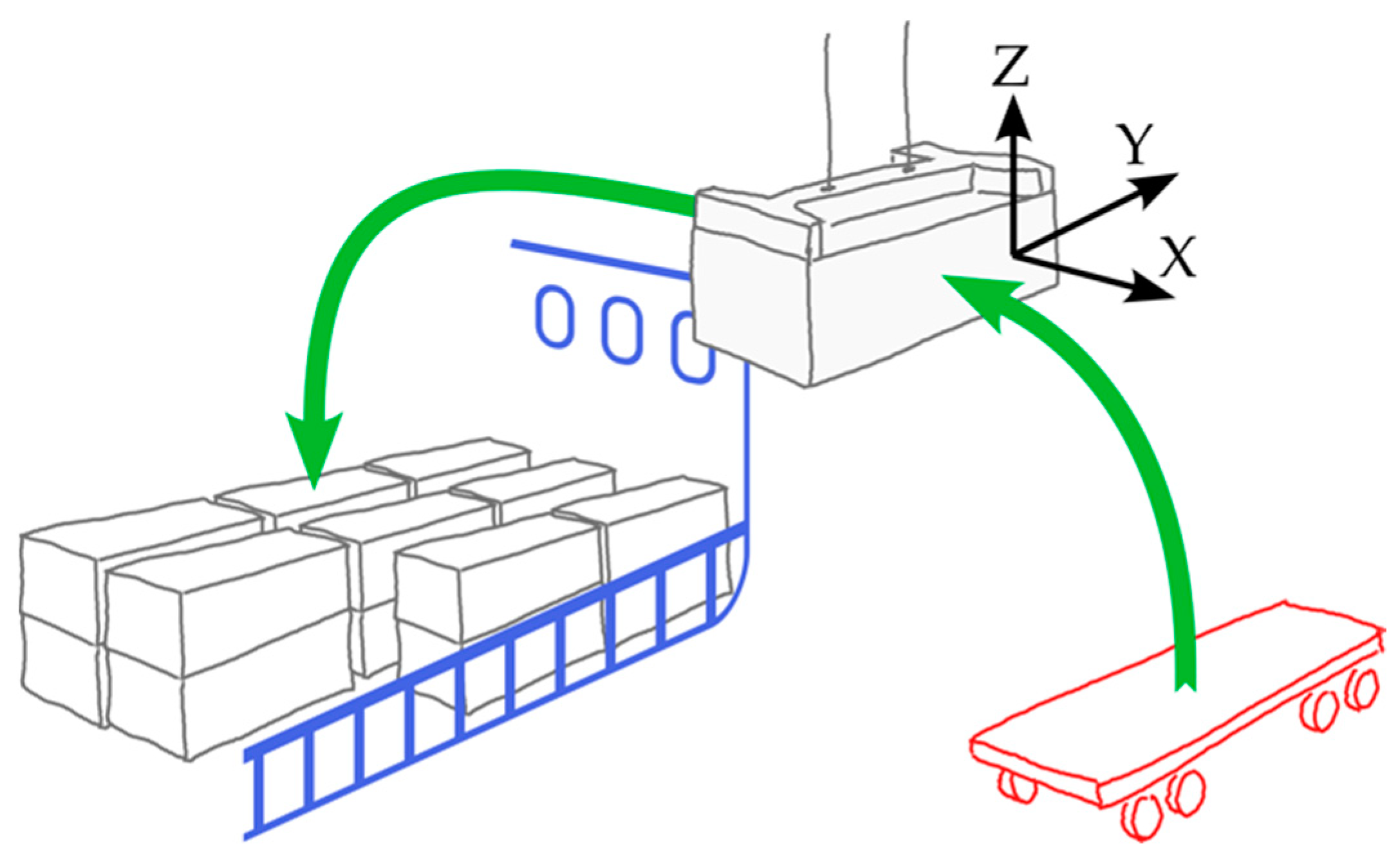
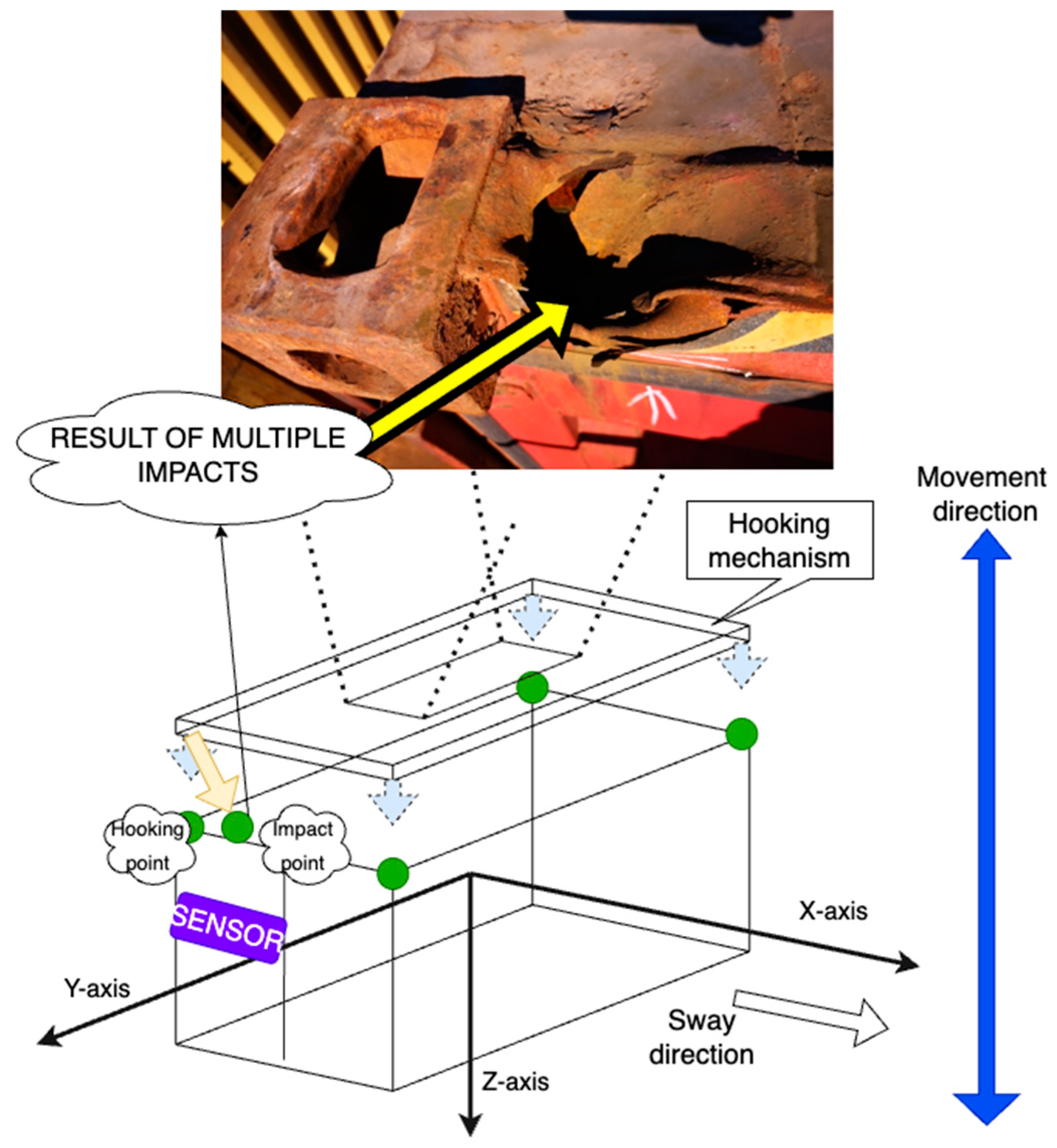
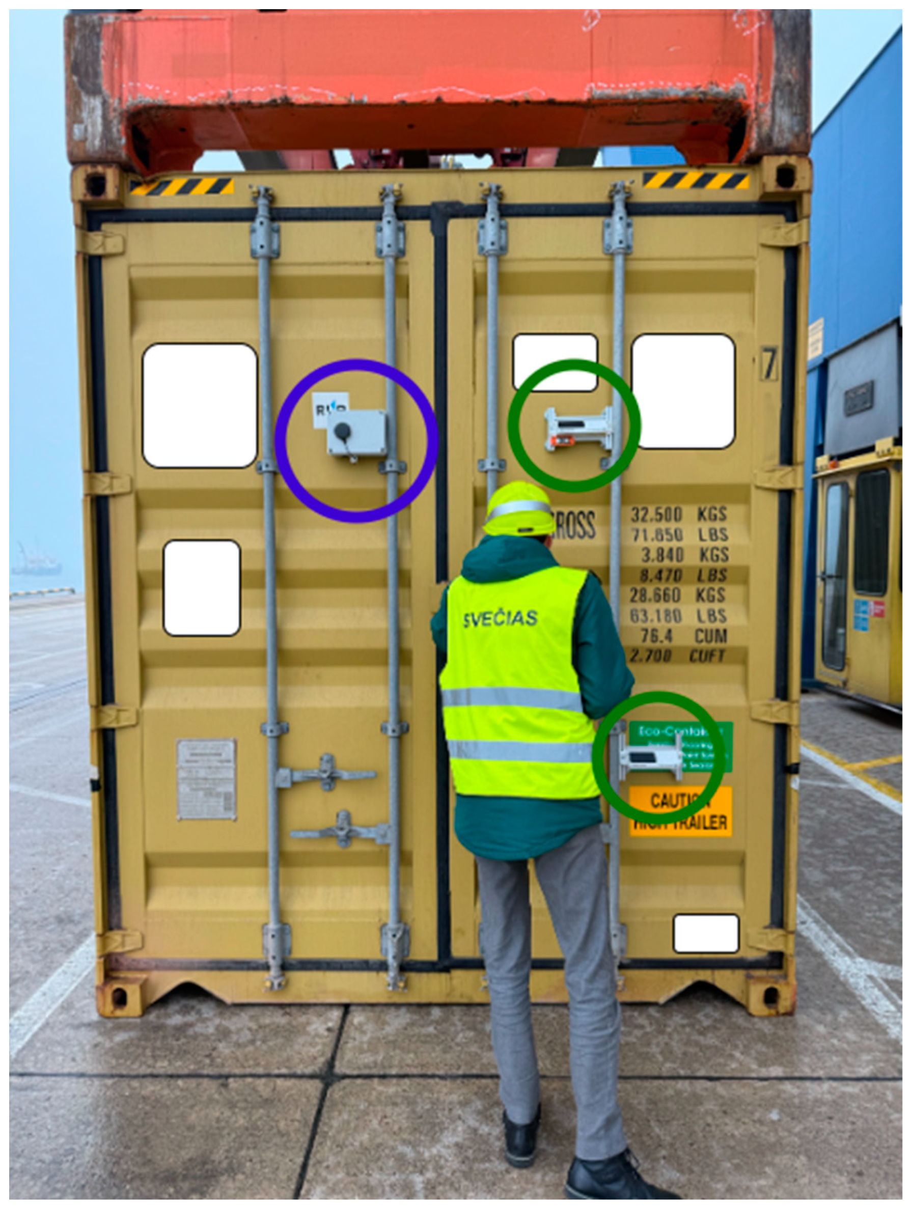
2.1. Description of the Experimental Setup

A critical step in the loading and unloading of containers, known as the handling procedure, involves attaching the containers to the crane’s spreaders and their further transportation either to the shore from the ship or vice versa (see Figure 1). This phase is particularly vulnerable to the generation of mechanical stresses and impacts. Such stresses typically arise from various factors, including abrupt crane movements, alignment discrepancies between the container and the spreader, and the substantial force exerted during the coupling of containers to the spreader bars. The mechanical impacts experienced during this operation can vary in severity.

They may present as minor vibrations, which could appear inconsequential; however, they have the potential to accumulate damage over time or as significant jolts that pose immediate risks to the integrity of the container and the safety of the operation, with incidents occurring in the shafts of the vessels. Each type of impact contributes differently to the potential degradation or damage of the container, as illustrated in Figure 2 (upper side).

This figure offers a visual representation of how these forces act upon the containers during the handling process, thereby providing a clearer understanding of the stresses involved. The probability of such damaging events is relatively high due to the complex and often expedited nature of port operations. Factors such as operator error, mechanical failure, environmental conditions, and improper container loading can exacerbate the likelihood of these occurrences. Despite advancements in crane technology and operational procedures, the risk of impact and subsequent damage to containers remains a persistent challenge [50]. The dangers of neglecting the mechanical stresses and impact events affecting containerised cargo handling operations are significant and multifaceted. When these stresses and impacts go unnoticed or unresolved, the damages incurred can severely compromise the structural integrity of containers. This endangers the safety of the cargo being transported and compromises the safety of personnel involved in subsequent handling, storage, and transportation activities.

Additionally, damaged containers can introduce a cascade of logistical challenges, including operational inefficiencies and delays, which may result in significant financial losses. These losses can stem from increased costs associated with damage claims, repairs, and replacements, as well as potential fines or penalties for non-compliance with safety regulations and standards. Given the high stakes, it becomes evident that there is an urgent need to develop a robust and reliable detection system capable of monitoring, identifying, and mitigating these risks proactively and efficiently. Such a system would play a critical role in ensuring the safety and structural integrity of containers while also streamlining operations and reducing the likelihood of unforeseen expenses and disruptions.

This proposed framework primarily revolves around an impact detection module prototype attached to the door side, as depicted in Figure 3, which was integral to the experimental setup used during the research.

The prototype incorporates a sophisticated data logging system equipped with fast local storage capabilities. Furthermore, the system features a data transmission module, allowing for the real-time collection and transmission of data related to impact events. The detection framework also integrates a range of advanced electronic components to enhance its functionality. The system underwent rigorous laboratory testing to validate its performance and reliability, which already demonstrated its potential [6]. During these tests, acceleration data and other critical parameters were collected using a scale model of a quay crane. The experimental setup involved installing the detection system on a specially prepared spreader subjected to varying loads and operational conditions during testing. This framework is expected to significantly improve safety standards, minimise costs, and ensure seamless cargo handling, contributing to more efficient and sustainable port operations. The device system consisted of the following:

• Data transmission unit using Bluetooth 5.1.
• Raspberry Pi 4 (four ARM A72 1.5 GHz cores, 8 GB of RAM) with a 128 GB SD UHS-I memory card.
• SINDT-232 digital accelerometer with high-stability 200 Hz MPU6050 3-axis acceleration (WitMotion Shenzhen Co., Ltd., Shenzhen, China), having 0.05-degree accuracy and an acceleration range of ±16 g.
• Inner 33,000 mAh battery.

A series of experimental hooking procedures were conducted as part of the study to evaluate the detection system under real-world operational conditions. These procedures were carefully carried out from the truck positioned below the quay crane, replicating typical container handling scenarios. Visual inspections were performed during each use case to ensure thoroughness and assess the condition and behaviour of the system under varying operational parameters, as outlined in the referenced study [6].

For each operation conducted during the experimental phase, two distinct datasets were collected to facilitate a comprehensive analysis of the detection system’s performance. The first dataset represented normal operations where no impact events were detected, serving as a baseline for comparison. The second dataset captured instances of actual impact events, highlighting the system’s ability to identify and document mechanical stresses and impact occurrences (see Figure 4).

By analysing these two datasets side by side, the research team evaluated the accuracy and reliability of the detection framework in distinguishing between normal operational conditions and scenarios involving significant impacts. This dual-dataset approach was instrumental in verifying the system’s effectiveness in real-world situations. It provided critical insights into its capacity to enhance safety and operational efficiency in container handling and transportation environments. Here, a “normal” operation with a small number of low-energy actual impacts is compared to a “noisy” operation with a higher count of impacts of higher energies, all for the X, Y, and Z axes. Also, a previously developed autoencoder integration technique (see Figure 5 [6]) was used again, as it has already proven its capability to work with the apparatus. We would like to highlight that existing container monitoring systems heavily rely on remote cloud processing, which can lead to latency issues, data loss, and a high degree of dependency on continuous network connectivity.

Current impact detection mechanisms are limited in capturing transient mechanical stresses in real time, often requiring post-event analysis based on incomplete datasets. Furthermore, traditional threshold-based anomaly detection methods struggle to distinguish actual impact events from operational vibrations, leading to frequent false positives. Our proposed edge-integrated framework directly processes impact data at the source, minimising latency, reducing dependence on external infrastructure, and improving detection accuracy.

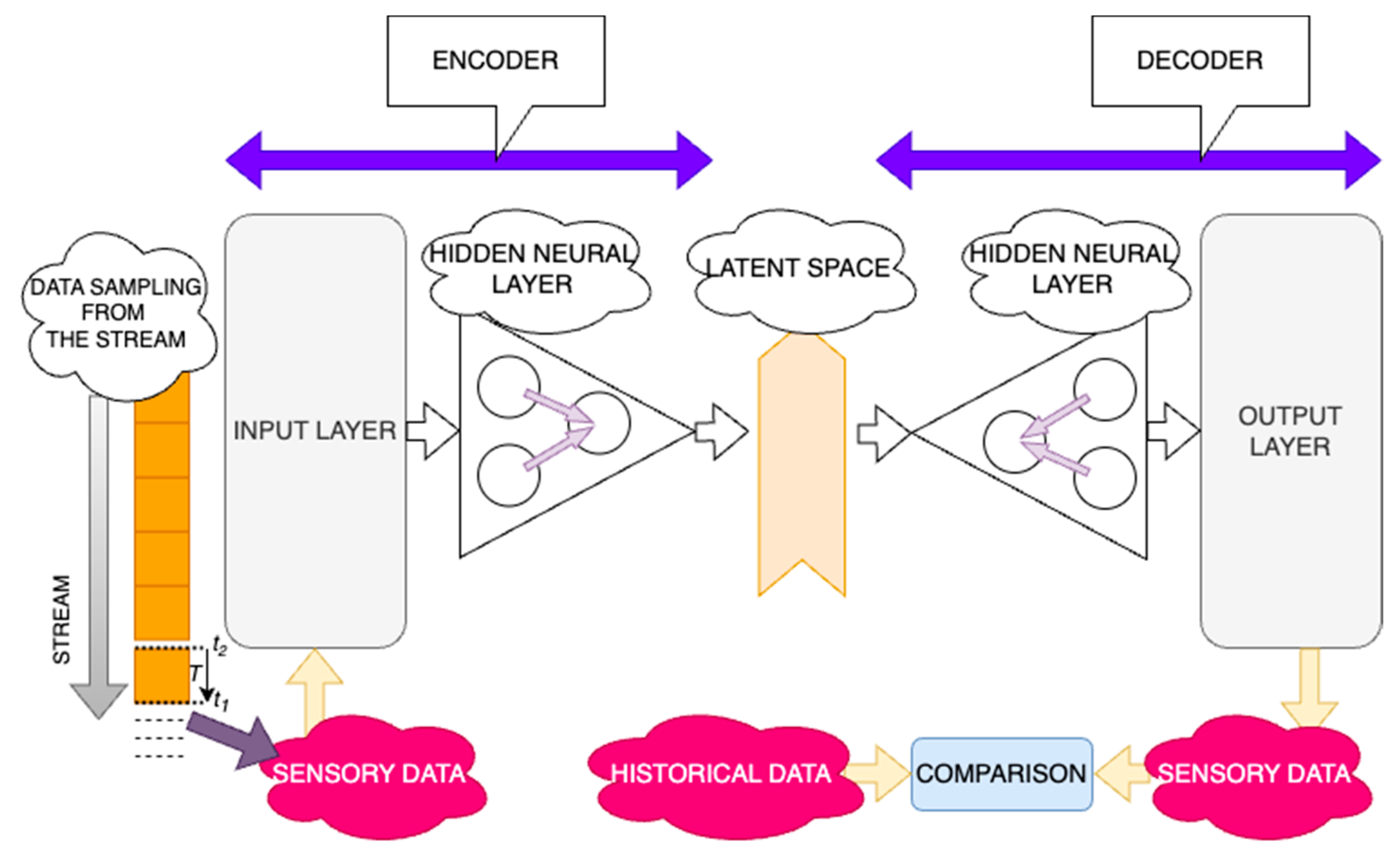
2.2. Structure of an Autoencoder

An unsupervised autoencoder is a type of neural network used for unsupervised learning of efficient coding, typically for dimensionality reduction or feature learning. The basic structure of an autoencoder can be described using Figure 6 and the mathematical expression involving its encoding and decoding functions.

An autoencoder consists of two main parts:

• Encoder: This part of the network compresses the input into a more miniature, encoded representation. The encoder function is typically denoted as $f$.
• Decoder: This part attempts to reconstruct the input from the encoded representation. The decoder function is typically denoted as $g$.

The mathematical expression is as follows: let $x\in {\mathbb{R}}^d$ be the input vector to the autoencoder. The encoding function $f$ maps this input to a hidden representation $z$ in a lower-dimensional space ${\mathbb{R}}^h$ (where typically $h<d$) (1):

$$z=f\left(x;{\theta }_e\right).$$

(1)

Here, ${\theta }_e$ represents the parameters of the encoder. The decoding function $g$ then attempts to reconstruct the original input from this hidden representation (2):

$$\widehat{x}=g\left(z;{\theta }_d\right).$$

(2)

Here, ${\theta }_d$ represents the parameters of the decoder.

The goal of the autoencoder is to minimise the difference between the input $x$ and its reconstruction $\widehat{x}$. This is often achieved by minimising a loss function $L$ over the parameters of the encoder and decoder $L\left(x,\widehat{x}\right)$. A common choice for $L$ is the mean squared error (MSE), which can be expressed as (3):

$$L\left(x,\widehat{x}\right)={‖x-\widehat{x}‖}^2.$$

(3)

Combining these, the complete operation of an autoencoder can be described by the following:

$$\widehat{x}=g\left(f\left(x;{\theta }_e\right);{\theta }_d\right).$$

(4)

The training involves optimising the following:

$${min}_{\left({\theta }_e,{\theta }_d\right)}{\sum }_{i=1}^{N}L\left(x^{\left(i\right)};{\widehat{x}}^{\left(i\right)}\right).$$

(5)

where $N$ is the number of training samples, and $x^{\left(i\right)}$ and ${\widehat{x}}^{\left(i\right)}$ are the i-th input and its reconstruction, respectively. This framework allows the autoencoder to learn valuable properties of the data unsupervised as it tries to capture the essential features necessary to reconstruct the input from the compressed encoded representation. When analysing time-series data using unsupervised learning methods, specific autoencoder architectures are well-suited to capture such data’s temporal dependencies and nuances. Here are two key types of autoencoders that are often employed in unsupervised time-series analytics:

• Recurrent Autoencoders (RAEs) utilise recurrent neural network (RNN) architec-tures, like Long Short-Term Memory (LSTM) or Gated Recurrent Units (GRUs), in both the encoder and decoder parts. These models are highly effective for time-series data due to their ability to maintain state or memory across time steps, capturing the dynamic temporal behaviour of the data.
  • Encoder: Processes the input time-series data and compresses it into a latent space representation. It typically consists of several layers of LSTM or GRU cells that process each time step sequentially, updating their internal state based on both the current input and the previously hidden state

    $$z_t=LSTM\left(x_t,h_{t-1}\right).$$

    (6)
  • Where $x_t$ is the input at a time $t$, $h_{t-1}$ is the hidden state from the previous time step, and $z_t$ is the output of the LSTM representing the encoded state.
  • Decoder: Starts from the latent representation and attempts to reconstruct the original time-series data over time. The decoder can also be a sequence of LSTM or GRU cells, which takes the latent representation and reconstructs the sequence, potentially in reverse order or from a condensed state (7).

    $${\widehat{x}}_t=LSTM\left(z_t,{\widehat{h}}_{t-1}\right).$$

    (7)
  • Here, ${\widehat{x}}_t$ represents the reconstructed output at time $t$, and ${\widehat{h}}_{t-1}$ is the hidden state from the previous time step in the decoder.
• Temporal Convolutional Autoencoders (TCAEs) utilise convolutional neural network (CNN) architectures specifically designed for sequence data, referred to as 1D CNNs. These models are beneficial for handling large datasets where capturing long-term dependencies explicitly with RNNs might be computationally expensive.
  • Encoder: Applies convolutional filters to the input sequence to extract features over multiple time steps simultaneously. This is performed using 1D convolutions that slide over the time dimension, capturing patterns and anomalies in the data (8).

    $$z=ReLU\left(W_e\ast x+b_e\right).$$

    (8)
  • Where ($\ast )$ denotes the convolution operation, $W_e$ and $b_e$ are the weights and biases of the convolutional layers, respectively, and ReLU is the activation function.
  • Decoder: Used to map the latent space back to the time-series data’s original dimensionality. This part of the network learns to reconstruct the time sequence from the compressed encoded features (9).

    $$\widehat{x}=ReLU\left(W_d\ast z+b_d\right).$$

    (9)

The essence of these autoencoders is that they can be trained on large datasets without labels, making them ideal for exploratory data analysis and preliminary data processing where supervised labels might not be available. The choice between recurrent and convolutional architectures often depends on the specific characteristics of the data and computational constraints, being the primary research intent for our device and aligning the descriptions of the Recurrent Autoencoder (RAE) and the Temporal Convolutional Autoencoder with the mathematical structure of the classic autoencoder model, as seen in

Table 1. Parameters for the RAE framework.

ENCODER:	DECODER:
Input: $x_t$ (where $t$ indexes time steps in the input time-series).	Input: $z_t$ (where $t$ indexes time steps in the input time-series).
Encoding Function: $f$.	Decoding Function: $g$.
Output: Latent representation $z_t$.	Output: Reconstructed output ${\widehat{x}}_t$.
We get the expression: $z_t=f\left(x_t;{\theta }_e\right)=LSTM\left(x_t,h_{t-1};{\theta }_e\right)$ Here, ${\theta }_e$ includes the weights and biases of the LSTM layers in the encoder.	We get the expression: ${\widehat{x}}_t=g\left(z_t;{\theta }_d\right)=LSTM\left(z_t,{\widehat{h}}_{t-1};{\theta }_d\right)$ Here, ${\theta }_d$ includes the weights and biases of the LSTM layers in the decoder.

and

Table 2. Parameters for the CNN framework.

ENCODER:	DECODER:
Input: $x_t$ (the entire time-series input).	Input: $\mathrm{z}$.
Encoding Function: $f$.	Decoding Function: $g$.
Output: Latent representation $z_t$.	Output: Reconstructed output $\widehat{x}$.
We get the expression: $z=f\left(x;{\theta }_e\right)=ReLU\left(W_e\ast x+b_e\right)$ $W_e$ and $b_e$ represent the weights and biases of the convolutional layers, respectively, and ($\ast$) denotes the convolution operation.	We get the expression: $\widehat{x}=g\left(z;{\theta }_d\right)=ReLU\left(W_d\ast z+b_d\right)$ $W_d$ and $b_d$ represent the weights and biases of the transposed convolutional layers, respectively.

.

In Table 1 and Table 2, we outline the hyperparameter choices for the RAE and TCAE models, detailing how each selection was made to optimise model performance. The learning rate, number of layers, and regularisation terms were chosen based on empirical testing, ensuring a balance between accuracy and computational efficiency. The performance comparison between RAEs and TCAEs provides valuable insights into the relative strengths of recurrent and convolutional architectures in impact detection, supporting our methodological approach. The most common objective in the Recurrent and Temporal Convolutional Autoencoders is to minimise the reconstruction error across the sequence ($L\left(x,\widehat{x}\right)).$ Where $x$ is the original input time-series, and $\widehat{x}$ is the reconstructed time-series output by the decoder. The training process involves optimising the parameters (${\theta }_e$ and ${\theta }_d$) to minimise the loss function $L$ over all the training samples. This can be achieved using standard backpropagation techniques tailored for time dependencies in RAEs and spatial feature extraction in convolutional architectures.

When employing autoencoders for time-series analysis, the goal is to minimise the loss function, quantifying the discrepancy between the input data and the reconstructed output from the model. The commonly used loss function in training autoencoders, particularly for time-series data, is the root mean squared error (RMSE). This function measures the squared root average of the squares of the differences between the original inputs and their reconstructed outputs. This is fundamental to ensuring that the autoencoder effectively learns the underlying patterns and dynamics of the data. Here is a detailed description of the minimisation of the loss function as a mathematical expression (10):

$$L\left(x,\widehat{x}\right)=\sqrt{{\displaystyle \frac{1}{T}}{\sum }_{t=1}^T{‖x-\widehat{x}‖}^2}.$$

(10)

where:

• $x_t$ is the input at time $t$.
• ${\widehat{x}}_t$ is the reconstruction output at time step $t$.
• $T$ is the total number of time steps in the time-series.
• ${‖·‖}^2$ denotes the squared Euclidian distance, ensuring that all errors are positive and that larger errors are penalized more heavily.

Concerning regularisation, it will prevent overfitting by adding a penalty term to the loss function. This penalty discourages overly complex models by penalising large weights. Regularisation techniques like L1 (Lasso: $\lambda \sum _i\left|{\theta }_i\right|)$ and L2 (Ridge: $\lambda \sum _i{{\theta }_i}^2$) add a penalty term to the loss function (11).

$$L\left(x,\widehat{x}\right)=\sqrt{{\displaystyle \frac{1}{T}}{\sum }_{t=1}^T{‖x-\widehat{x}‖}^2+\left\{\begin{array}{c}\lambda \sum _i\left|{\theta }_i\right|,or\\ \lambda \sum _i{{\theta }_i}^2\end{array}\right.}.$$

(11)

where:

• $\lambda$ is the regularisation strength.
• $\left|{\theta }_i\right|$ is the absolute value of each weight in the network.
• ${{\theta }_i}^2$ is the square of each weight in the network.

L1 regularisation encourages sparsity in the model weights, potentially leading to models that rely on fewer features. At the same time, L2 regularisation discourages large weights by penalising the square values of the weights, leading to a more evenly distributed importance across all features. Therefore, the objective function for training an autoencoder is to minimise the total reconstruction error over all instances in the training dataset (12):

$${min}_{{\theta }_e,{\theta }_d}\sqrt{{\displaystyle \frac{1}{N}}{\sum }_{i=1}^{N}L\left(x^{\left(i\right)},{\widehat{x}}^{\left(i\right)}\right)}.$$

(12)

where:

• $N$ is the number of training samples.
• ${\theta }_e$ and ${\theta }_d$ are the encoder and decoder parameters, respectively.

3. Results and Discussions

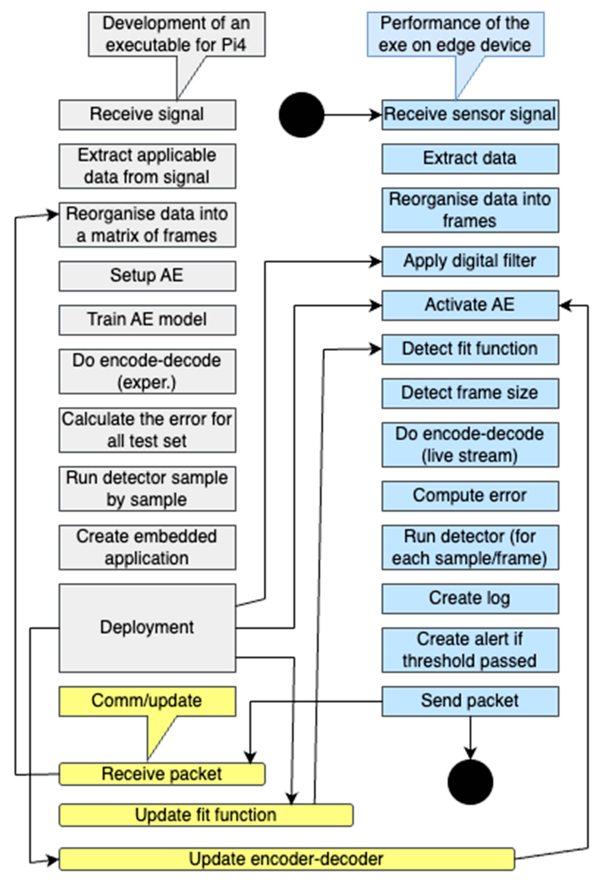
3.1. Data Preparation and Analytical Steps

The following steps were taken to enhance the predictive accuracy and reliability of the anomaly detection:

• Data Preparation. Container acceleration data is gathered using a single sensor. This data includes noise components, often seen as groups of anomalous outliers that compromise functional stability. To address this, the data is segmented into a training set, a validation set that contains only normal, extracted data, and a test set that includes both normal and anomalous data.
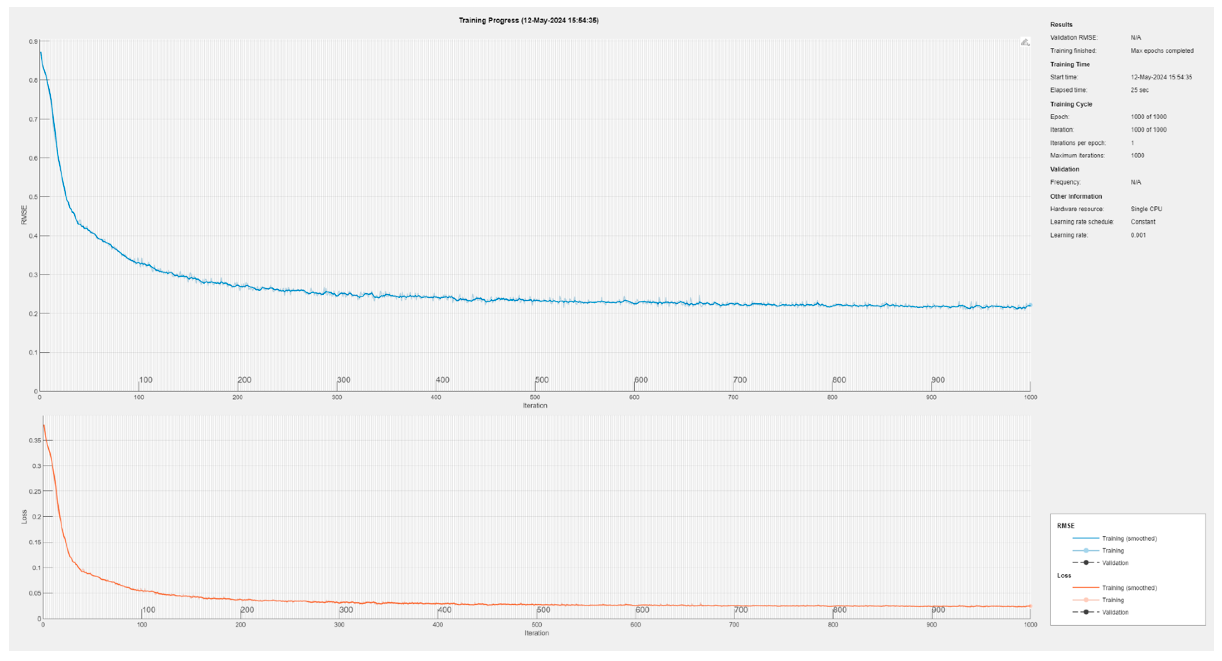
• Model Initialisation. The initial setup involves configuring the model’s hyperparameters, such as the weight coefficient, learning rate, number of iterations, and structure of the AE (autoencoder) module. At this stage of the experiment, the learning parameters were set to random values and optimised during the research process.
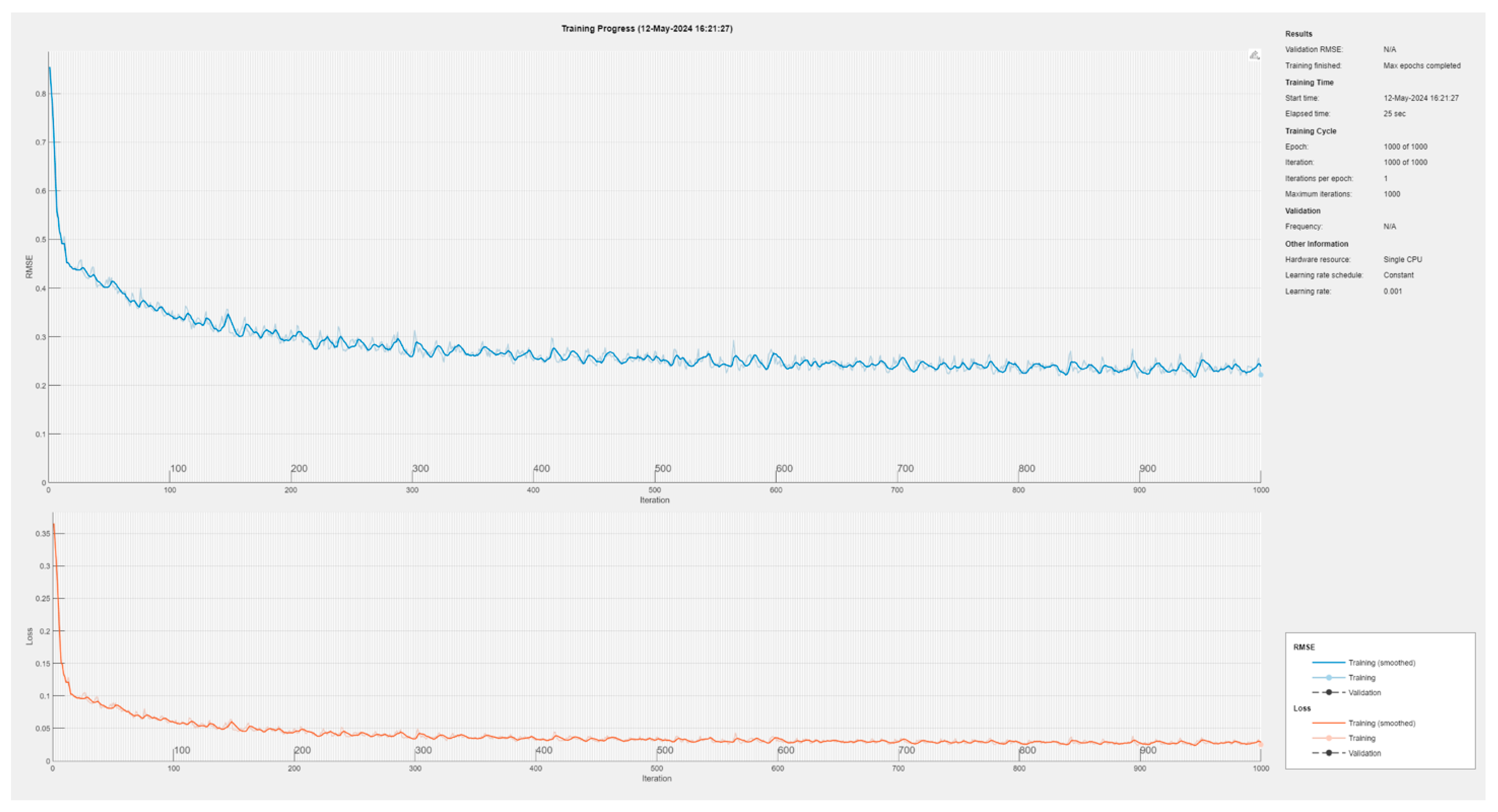
• Model Offline Training. The training process began by inputting only the normal data into the AE. Encoder fitting networks are then trained, leading to the generation of reconstructed data based on predefined equations. RMSE loss values are calculated during training, and the learning parameters of the network are updated iteratively, refining the model’s accuracy.
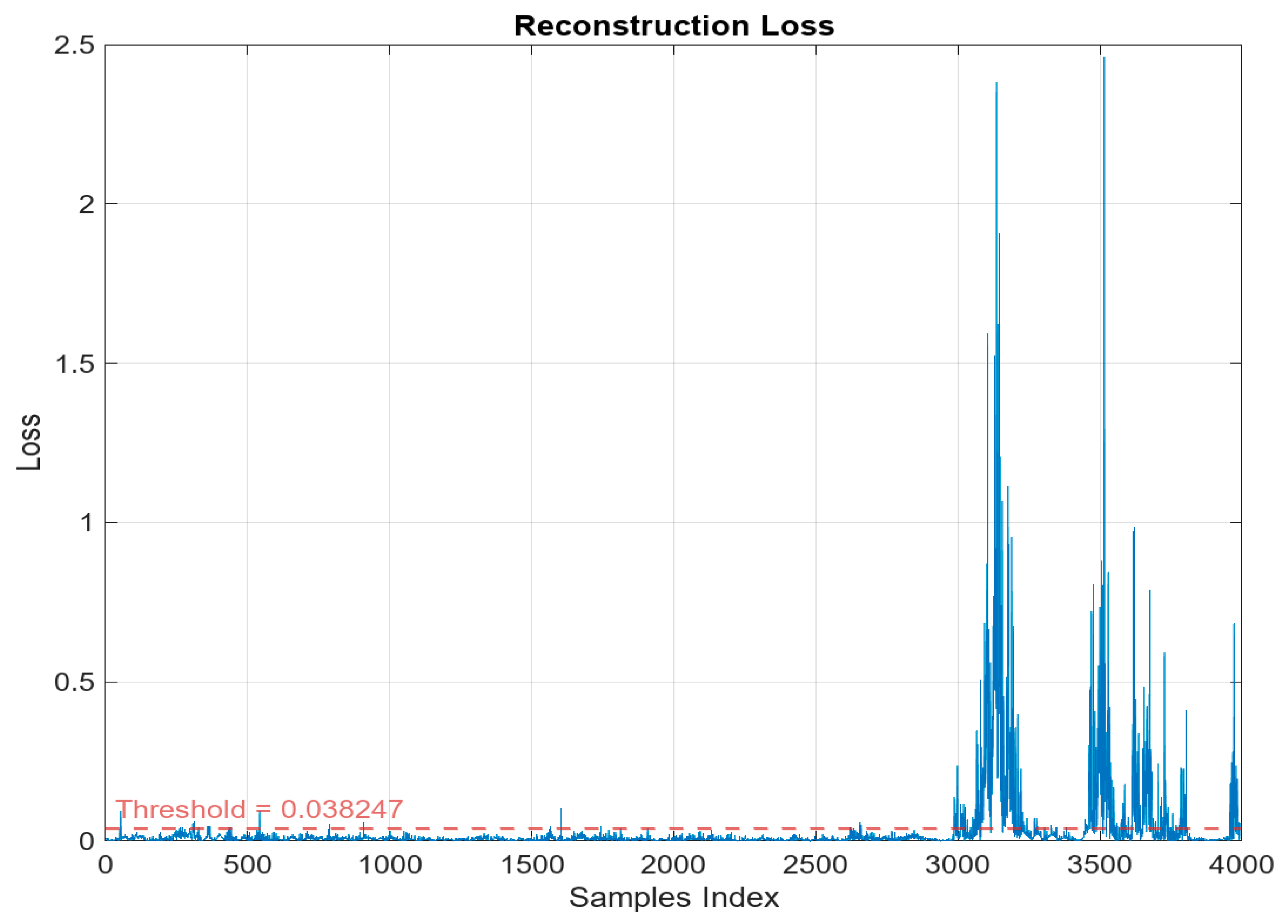
• Model Online Validation. In this phase, only the normal data from the validation set is processed through the trained network. After reconstructing this data, the combined loss values of RMSE for each sample are computed. Given the potential presence of a few unmatched noise samples and to ensure the model’s robustness, the loss value representing 95% of the normal data is selected as the threshold for detecting true anomalies (anomalous regions).
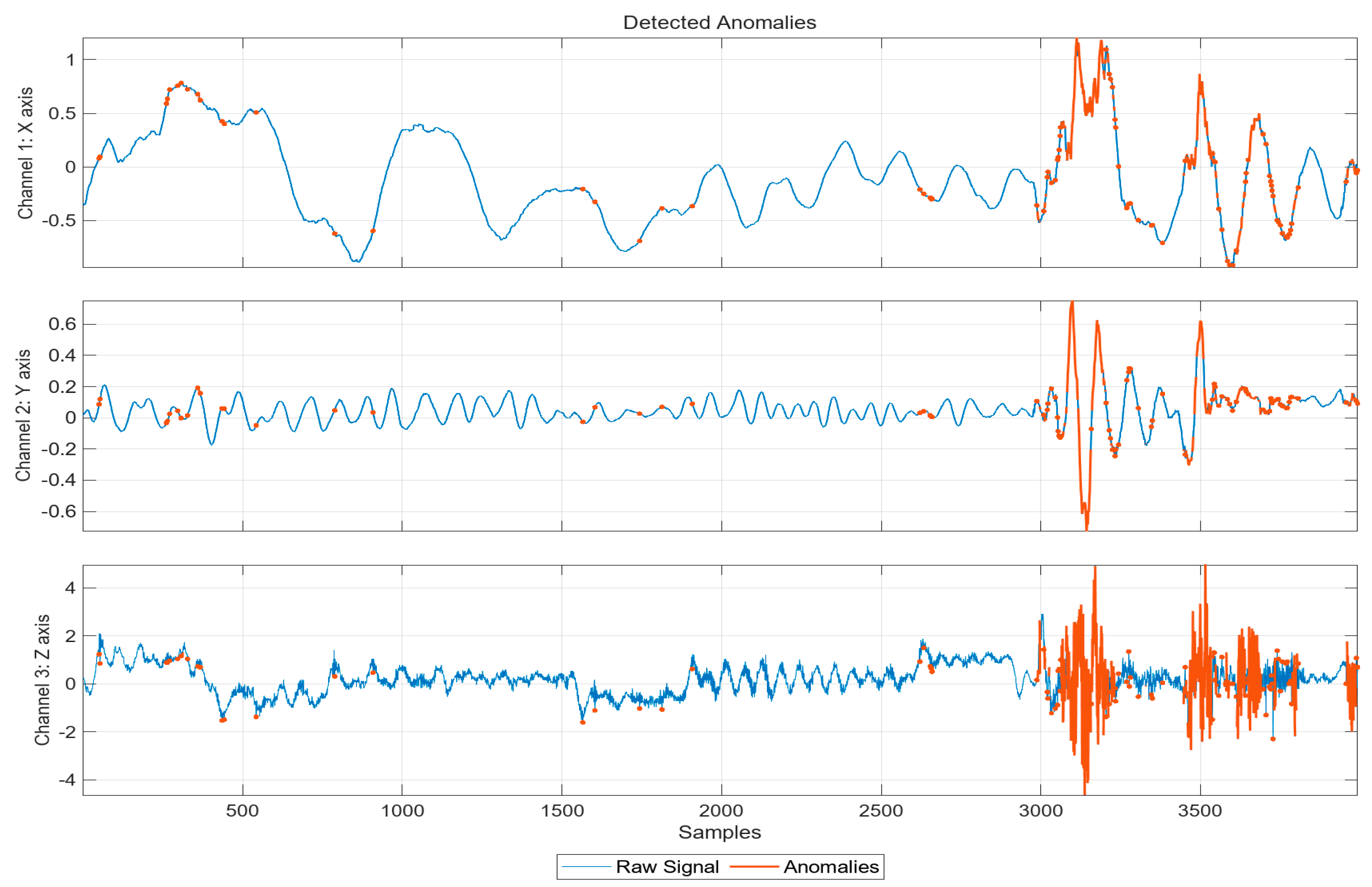
• Model Online Testing. The testing phase involves feeding both normal and anomalous data from the test set into the trained AE. The total RMSE loss values are then computed for each sample to categorise them as normal or anomalous based on the established threshold.

The dataset used in this study was collected under varying operational conditions, including different crane speeds and impact magnitudes. To enhance the robustness of the model, we implemented a preprocessing pipeline that included:

• Outlier detection and removal based on statistical thresholds.
• Linear interpolation to handle missing sensor data.
• Low-pass filtering to reduce high-frequency noise.

These preprocessing steps ensure that the autoencoder models are trained on a dataset that closely represents real-world conditions without distortions caused by spurious data artefacts. A detailed comparison of the core architecture and training parameters for both models is presented in

Table 3. Structural and training parameter comparison between the RAE and TCAE.

Parameter	RAE	TCAE-CN
Input shape	Flattened multivariate time window	Multivariate time sequence
Encoder	3 Dense layers (128 → 64 → 32)	2 Conv1D layers (32, 16 filters)
Decoder	3 Dense layers (64 → 128 → output)	Conv1D Transpose + Dense reconstruction
Latent dimension	32
Activation function	ReLU (hidden), Linear (output)	ReLU (hidden), Linear (output)
Loss function	Mean Squared Error (MSE)	MSE
Optimiser	Adam	Adam
Epochs	100	100

, highlighting the key difference between the RAE and the temporal convolutional design of the TCAE.

3.2. Computational Results Assessment

The initial findings suggest that the use of autoencoders is an up-and-coming innovation. The computational module successfully captured the acceleration of the spreader without any noticeable deviations and computed the CNN and RAE algorithms with the desired data sample size (up to 2 s). We assess unsupervised anomaly detection techniques using data subjected to high noise levels, with a specific focus on the Recurrent Autoencoder (RAE) and the Temporal Convolutional Autoencoder. In this study, we replicate all methods ten times to minimise the stochastic variability inherent in experiments. The algorithms simulating the operational conditions of the device are executed on MATLAB R2020b Update 3 for macOS version 14.4.1, utilising an M3 Max 14-core CPU and 36 GB of rapid memory. By managing variables, we aim to identify an optimal combination of hyperparameters by employing a greedy algorithm approach. The primary hyperparameters are configured as follows: the number of iterations is 1000; the learning rate is initially 0.01, with a decay factor of 0.1 after every 20 iterations; and the hyperparameter $\lambda$ in the loss function is set at 0.2 with L1. The selection of these hyperparameters is built on existing research and case studies.

Initial results for the handling operation mentioned in Section 2 are promising, as both frameworks were successfully deployed and worked as planned—both the RAE and CNN proved to work efficiently in detecting anomalous regions along the data stream without any severe computational strain on the device (see Figure 7 and Figure 8), sending obvious impact alerts during observable physical contacts (red dots) in the shafts of the ship’s hull (which tend to happen regularly [51]) after the 3000th sample. The red lines indicate the anomalous region on the graph, which is crucial for estimating the critical duration. For experimental clarity, computational rechecks were made for each use case to check the credibility of the results.

In Figure 7 and Figure 8, the red dots represent detected impact events based on the anomaly scores generated by the autoencoder models. These points indicate instances where the model identified deviations from standard operational patterns, marking cases of potential impact. The surrounding regions on the plots highlight the statistical distribution of impact-related anomalies over time, reinforcing the validity of our approach. During the initial stages of the operation, the detection algorithm identified several impacts, represented by red dots, even though these occurred during movements with no visible obstacles. This indicates that the algorithm made several false assumptions about the presence of impacts in these scenarios. However, it is noteworthy that despite these false positives, the algorithm was able to assess the statistical significance of these detected impacts and determined them to be of low importance. As a result, no anomalous regions were generated based on these false detections. This outcome highlights a key strength of the detection system: its ability to effectively distinguish between actual impact events and false positives, ensuring that only genuinely significant impacts contribute to the formation of anomalous regions. This is the desired output of the experiment, as it demonstrates the capability of the solution to prioritise and correctly identify meaningful events.

Furthermore, a detailed analysis of the system’s performance revealed that the Recurrent Autoencoder (RAE) proved to be a slightly superior solution when evaluated using reconstruction loss estimates (see Figure 9 and Figure 10). The RAE’s ability to consistently achieve lower reconstruction loss values under experimental conditions indicates its effectiveness in handling the complexities of impact detection and distinguishing between normal operational data and anomalous data points.

Additionally, the comparative analysis of the reconstruction loss distribution between normal operations and operations with identified physical impacts (see Figure 10 and Figure 11) further validates the RAE’s robustness. This analysis underscores its potential as a reliable tool for distinguishing actual physical impacts from noise or false positives, thereby enhancing the overall accuracy and reliability of the detection framework. By demonstrating these capabilities, the RAE highlights its value as an integral component of the proposed detection system, contributing to the successful implementation of an efficient and accurate monitoring solution for container handling operations.

Figure 11 and Figure 12 present the reconstruction loss distributions for the CNN and RAE frameworks. Both models effectively differentiate normal operations from impact-related anomalies, but the Recurrent Autoencoder (RAE) exhibits a more precise separation between these two categories. This improved separation suggests that the RAE is more capable of capturing temporal dependencies in impact signals, leading to reduced false positive rates.

In contrast, the Temporal Convolutional Autoencoder (TCAE) framework shows a slight overlap between normal and anomaly loss distributions, which may increase the likelihood of missed impact events (false negatives). The superior performance of the RAE in distinguishing between normal and impact conditions supports its practical applicability for real-time impact monitoring in port operations. Comparative analysis of the RMSE curves, as well as the loss function during the training period, shows that the RAE performs sufficiently better under the experimental conditions of 1000 computing iterations (see Figure 13 and Figure 14), indicating that the number of iterations may be diminished up to 300, thus lowering the computational strain on the edge device and increasing the response time of the system.

This observed performance suggests that the RAE is highly effective at minimising error rates and optimising the loss function, even in demanding experimental setups. Interestingly, the analysis also reveals that the number of computational iterations required for satisfactory performance can be significantly reduced from 1000 to as few as 300 iterations. This adjustment is particularly advantageous, as it would substantially lower the computational strain on the edge device where the detection system is deployed. The system becomes more efficient by reducing its computational load, resulting in a shorter response time and improved real-time operational capabilities. These improvements ensure the effectiveness of the detection framework in dynamic, time-sensitive environments, such as port container operations, where rapid and accurate responses are crucial for maintaining safety and operational efficiency. In addition to RMSE, we evaluated the performance of our anomaly detection models using Precision, Recall, and F1-score to provide a more comprehensive assessment of their ability to distinguish true impacts from false positives. RMSE serves as a helpful metric for measuring the reconstruction loss in autoencoders, but it does not provide a direct indication of classification accuracy. Precision was included to assess the proportion of detected anomalies that were actual impact events, while Recall measured the model’s ability to identify all impact occurrences correctly. The F1-score, as a harmonic mean of Precision and Recall, ensured a balanced evaluation of the model’s detection capability. The Recurrent Autoencoder (RAE) demonstrated superior anomaly detection performance, achieving a Precision of 91.3%, a Recall of 87.6%, and an F1-score of 89.4%. Comparatively, the Temporal Convolutional Autoencoder (TCAE) exhibited a Precision of 89.5%, a Recall of 85.2%, and an F1-score of 87.3%. While both models effectively detected physical impacts, the RAE outperformed the TCAE in capturing sequential dependencies within the time-series data, resulting in fewer missed anomalies. To further validate our results, we analysed the RMSE values for detected anomalies and everyday operations. The mean RMSE for actual impact events was 0.124, whereas the mean RMSE for normal operational conditions remained at 0.069. This distinct separation confirms the effectiveness of the autoencoder-based anomaly detection framework. Additionally, we considered alternative threshold selection methods, including interquartile range filtering and adaptive thresholding based on local statistical properties, both of which reinforced the robustness of our chosen threshold, specifically the 95th percentile root mean squared error (RMSE).

Initial false positives were primarily attributed to transient vibrations during crane acceleration and deceleration phases. These vibrations produced signal variations that closely resembled minor impact events. To mitigate this, we refined our anomaly detection approach by introducing a time-based impact validation step, ensuring that only consecutive anomalies exceeding a predefined duration threshold were classified as actual impacts. Additionally, applying a contextual verification method, where detected anomalies were cross-checked against operational parameters such as crane velocity, further reduced false favourable rates.

The proposed impact detection framework represents a significant advancement in real-time anomaly detection for container handling. By integrating autoencoders within edge computing units, our approach enables proactive damage assessment, reducing operational delays and maintenance costs. The findings of this study provide a foundation for future enhancements in intelligent container tracking systems, with potential applications extending to automated ports and intelligent logistics networks.

In comparison to existing studies in the field, our proposed edge-integrated autoencoder framework demonstrates superior performance in both detection accuracy and deployment feasibility. While various studies have explored the use of autoencoders for anomaly detection, these are often evaluated under controlled conditions or with post-processing on centralised servers. In contrast, our system achieved an F1-score of 89.4% and a recall of 87.6% directly on embedded hardware deployed in a working port terminal, demonstrating robustness in the presence of high mechanical noise and stochastic operational variability. Unlike approaches that rely on offline analysis or cloud-based inference, our solution processes data on-device using lightweight RAE and TCAE architectures implemented on a Raspberry Pi-class processor. This addresses a key challenge in edge AI deployment, balancing computational cost with real-time reliability. To our knowledge, no previous study has systematically evaluated both recurrent and convolutional autoencoder models in the context of quay crane operations, positioning this work as a methodological advancement in unsupervised learning for maritime logistics. Additional comparative analysis of AE adoption in edge computing applications suggests that our solution has much room for improvement (see

Table 4. Comparative analysis of several edge computing applications using various AE solutions.

Paper	AE Type	F1-Score	Edge Device	Notes
This research	RAE-TCAE	RAE 0.894	Raspberry Pi 4	Low-cost, high recall
Adversarial AE for IoT Intrusion [52]	Adv-AE + KNN	0.999	Raspberry Pi 3B	High performance
Lightweight LAE in Poultry Farm [46]	LSTM-LAE	0.963	Raspberry Pi 4	Low-cost, high recall

).

While previous works have explored autoencoders in various industrial settings, few have evaluated their effectiveness under dynamic quay crane operations, and none, to our knowledge, have directly compared recurrent and convolutional architectures in such a context. This positions our work as both a methodological and practical advancement in the application of unsupervised learning for maritime logistics.

This work represents a significant advancement in the field of transport engineering by introducing ongoing research on the use of autoencoders for real-time anomaly identification in sensor data. It describes the architecture and deployment of an edge sensor-integrated anomaly detection system. The autoencoder-based approach has undergone extensive testing in an operating environment. These technologies are especially helpful in preventing severe damage to containers and cargo by promptly alerting managers, crane operators, and port maintenance workers.

4. Conclusions

Regarding the limitations and challenges, as well as future research agendas:

• Local Minima and Non-Convexity. The loss function of deep autoencoders is typically non-convex due to the complex nature of neural networks and their complex deployment. This leads to potential issues where the optimisation algorithm might converge to a local minimum rather than the global minimum, depending on the initial hyperparameter values.
• Overfitting. Autoencoders can be overfit to training data, especially if:
  • The network architecture is too complex relative to the amount of input data.
  • The selected framework model’s capacity is too high, allowing the network to learn both pertinent features and noise in the training data.
• Sensitivity to Hyperparameters. The performance of the autoencoder is influenced by the selection of hyperparameters, including the number of layers, the number of neurons in each layer, the types of layers (e.g., convolutional, recurrent), the learning rate, and the optimisation algorithm employed.
• Balancing Encoder and Decoder Strength. A balance is needed between the encoder’s and decoder’s capacities. An overly powerful encoder or decoder can skew the learning process, leading to poor generalisation.
• The Dimensionality of Latent Space. The choice of the dimensionality of the latent space is crucial. Too large a latent space might lead the model to learn an identity function, where it can simply copy the input to the output without proper data compression. Conversely, a latent space that is too small may not capture all the necessary features of the data.

To support the claim of edge suitability, we evaluated the computational performance of the proposed models on the Raspberry Pi 4 (8 GB RAM), which served as our embedded deployment platform. Both the Recurrent Autoencoder (RAE) and the Temporal Convolutional Autoencoder (TCAE) were successfully executed on-device without noticeable delays during real-time data capture and inference. Preliminary testing showed that model inference for individual time-series samples (2-second windows at 200 Hz) completes within a fraction of a second, with no disruption to data logging or transmission processes. Resource usage remained within acceptable limits for real-time embedded applications, and the system operated continuously without thermal throttling or instability. While a detailed power and latency profile was not within the scope of this study, the results demonstrate that the selected autoencoder architectures can operate effectively within the computational constraints of commonly available edge hardware, confirming their practical viability for deployment in container impact monitoring scenarios.

We recognise that the experimental dataset used in this study was collected under controlled conditions at a single container terminal using a specific quay crane configuration. While the system demonstrated promising results in detecting mechanical impacts in this setting, its applicability to other operational environments, such as different crane types, port layouts, or environmental conditions (e.g., weather variability, structural vibration patterns, or loading speeds), has not yet been verified. Variations in crane dynamics, spreader mechanisms, and container suspension systems may significantly influence sensor outputs, potentially affecting model sensitivity and false-positive rates. To address this limitation, future research will focus on multi-site validation across various terminals and geographic locations. This includes testing with diverse crane types (e.g., ship-to-shore cranes, rubber-tyred gantries) and under various real-world environmental conditions to ensure robustness, reduce susceptibility to site-specific overfitting, and enhance model adaptability for widespread deployment.

Additionally, upcoming work will explore scaling autoencoder architectures to accommodate larger datasets, optimising computational efficiency for deployment on ultra-low-power IoT platforms and integrating context-aware features such as predictive maintenance analytics. We also aim to develop adaptive learning mechanisms that allow the system to dynamically adjust hyperparameters based on changing environmental inputs, thus maintaining consistent performance across operational scenarios. Although the current implementation demonstrates strong real-world potential, further experimentation involving deeper and more varied encoder–decoder structures is necessary to maximise detection accuracy and resilience in diverse logistical settings.

References

1. Rashid, N.; Hossain, M.A.F.; Ali, M.; Islam Sukanya, M.; Mahmud, T.; Fattah, S.A. AutoCovNet: Unsupervised Feature Learning Using Autoencoder and Feature Merging for Detection of COVID-19 from Chest X-Ray Images. Biocybern. Biomed. Eng. 2021, 41, 1685–1701. [Google Scholar] [CrossRef] [PubMed]
2. Du, X.; Yu, J.; Chu, Z.; Jin, L.; Chen, J. Graph Autoencoder-Based Unsupervised Outlier Detection. Inf. Sci. 2022, 608, 532–550. [Google Scholar] [CrossRef]
3. Ali, S.; Li, Y. Learning Multilevel Auto-Encoders for Ddos Attack Detection in Smart Grid Network. IEEE Access 2019, 7, 108647–108659. [Google Scholar] [CrossRef]
4. Hong, S.; Kang, M.; Kim, J.; Baek, J. Investigation of Denoising Autoencoder-Based Deep Learning Model in Noise-Riding Experimental Data for Reliable State-of-Charge Estimation. J. Energy Storage 2023, 72, 108421. [Google Scholar] [CrossRef]
5. Saetta, E.; Tognaccini, R.; Iaccarino, G. Uncertainty Quantification in Autoencoders Predictions: Applications in Aerodynamics. J. Comput. Phys. 2024, 506, 112951. [Google Scholar] [CrossRef]
6. Jakovlev, S.; Voznak, M. Auto-Encoder-Enabled Anomaly Detection in Acceleration Data: Use Case Study in Container Handling Operations. Machines 2022, 10, 734. [Google Scholar] [CrossRef]
7. Cha, S.-H.; Noh, C.-K. A Case Study of Automation Management System of Damaged Container in the Port Gate. J. Navig. Port. Res. 2017, 41, 119–126. [Google Scholar] [CrossRef]
8. Wang, Z.; Gao, J.; Zeng, Q.; Sun, Y. Multitype Damage Detection of Container Using CNN Based on Transfer Learning. Math. Probl. Eng. 2021, 2021, 115022. [Google Scholar] [CrossRef]
9. Park, H.; Lee, G.H.; Han, J.; Choi, J.K. Multiclass Autoencoder-Based Active Learning for Sensor-Based Human Activity Recognition. Future Gener. Comput. Syst. 2024, 151, 71–84. [Google Scholar] [CrossRef]
10. Yang, Z.; Xu, B.; Luo, W.; Chen, F. Autoencoder-Based Representation Learning and Its Application in Intelligent Fault Diagnosis: A Review; Elsevier Ltd.: Amsterdam, The Netherlands, 2021; ISBN 8675523256054. [Google Scholar]
11. Santhi, T.M.; Srinivasan, K. A Duo Autoencoder-SVM Based Approach for Secure Performance Monitoring of Industrial Conveyor Belt System. Comput. Chem. Eng. 2023, 177, 108359. [Google Scholar] [CrossRef]
12. Zheng, S.; Zhao, J. A New Unsupervised Data Mining Method Based on the Stacked Autoencoder for Chemical Process Fault Diagnosis. Comput. Chem. Eng. 2020, 135, 106755. [Google Scholar] [CrossRef]
13. Lv, L.; Bardou, D.; Liu, Y.; Hu, P. Deep Autoencoder-like Non-Negative Matrix Factorization with Graph Regularized for Link Prediction in Dynamic Networks. Appl. Soft Comput. J. 2023, 148, 110832. [Google Scholar] [CrossRef]
14. Sarıkaya, A.; Kılıç, B.G.; Demirci, M. RAIDS: Robust Autoencoder-Based Intrusion Detection System Model Against Adversarial Attacks. Comput. Secur. 2023, 135, 103483. [Google Scholar] [CrossRef]
15. Wang, J.; Xie, X.; Shi, J.; He, W.; Chen, Q.; Chen, L.; Gu, W.; Zhou, T. Denoising Autoencoder, A Deep Learning Algorithm, Aids the Identification of A Novel Molecular Signature of Lung Adenocarcinoma. Genom. Proteom. Bioinform. 2020, 18, 468–480. [Google Scholar] [CrossRef]
16. Dumais, F.; Legarreta, J.H.; Lemaire, C.; Poulin, P.; Rheault, F.; Petit, L.; Barakovic, M.; Magon, S.; Descoteaux, M.; Jodoin, P.-M. FIESTA: Autoencoders for Accurate Fiber Segmentation in Tractography. Neuroimage 2023, 279, 120288. [Google Scholar] [CrossRef]
17. Takhanov, R.; Abylkairov, Y.S.; Tezekbayev, M. Autoencoders for a Manifold Learning Problem with a Jacobian Rank Constraint. Pattern Recognit. 2023, 143, 109777. [Google Scholar] [CrossRef]
18. Tsakiridis, N.L.; Samarinas, N.; Kokkas, S.; Kalopesa, E.; Tziolas, N.V.; Zalidis, G.C. In Situ Grape Ripeness Estimation via Hyperspectral Imaging and Deep Autoencoders. Comput. Electron. Agric. 2023, 212, 108098. [Google Scholar] [CrossRef]
19. Yang, H.; Ding, W.; Yin, C. AAE-Dpeak-SC: A Novel Unsupervised Clustering Method for Space Target ISAR Images Based on Adversarial Autoencoder and Density Peak-Spectral Clustering. Adv. Space Res. 2022, 70, 1472–1495. [Google Scholar] [CrossRef]
20. Cai, L.; Li, J.; Xu, X.; Jin, H.; Meng, J.; Wang, B.; Wu, C.; Yang, S. Automatically Constructing a Health Indicator for Lithium-Ion Battery State-of-Health Estimation via Adversarial and Compound Staked Autoencoder. J. Energy Storage 2024, 84, 110711. [Google Scholar] [CrossRef]
21. Liu, Z.; Teka, H.; You, R. Conditional Autoencoder Pricing Model for Energy Commodities. Resour. Policy 2023, 86, 104060. [Google Scholar] [CrossRef]
22. Wang, W.; Wang, H.; Chen, L.; Hao, K. A Novel Soft Sensor Method Based on Stacked Fusion Autoencoder with Feature Enhancement for Industrial Application. Measurement 2023, 221, 113491. [Google Scholar] [CrossRef]
23. Xiao, D.; Qin, C.; Yu, H.; Huang, Y.; Liu, C.; Zhang, J. Unsupervised Machine Fault Diagnosis for Noisy Domain Adaptation Using Marginal Denoising Autoencoder Based on Acoustic Signals. Measurement 2021, 176, 109186. [Google Scholar] [CrossRef]
24. Yang, H.; Qiu, R.C.; Shi, X.; He, X. Unsupervised Feature Learning for Online Voltage Stability Evaluation and Monitoring Based on Variational Autoencoder. Electr. Power Syst. Res. 2020, 182, 106253. [Google Scholar] [CrossRef]
25. Yan, S.; Shao, H.; Xiao, Y.; Liu, B.; Wan, J. Hybrid Robust Convolutional Autoencoder for Unsupervised Anomaly Detection of Machine Tools under Noises. Robot. Comput. Integr. Manuf. 2023, 79, 102441. [Google Scholar] [CrossRef]
26. Buzuti, L.F.; Thomaz, C.E. Fréchet AutoEncoder Distance: A New Approach for Evaluation of Generative Adversarial Networks. Comput. Vision. Image Underst. 2023, 235, 103768. [Google Scholar] [CrossRef]
27. Mulyanto, M.; Leu, J.S.; Faisal, M.; Yunanto, W. Weight Embedding Autoencoder as Feature Representation Learning in an Intrusion Detection Systems. Comput. Electr. Eng. 2023, 111, 108949. [Google Scholar] [CrossRef]
28. Danti, P.; Innocenti, A. A Methodology to Determine the Optimal Train-Set Size for Autoencoders Applied to Energy Systems. Adv. Eng. Inform. 2023, 58, 102139. [Google Scholar] [CrossRef]
29. Zhu, J.; Deng, F.; Zhao, J.; Chen, J. Adaptive Aggregation-Distillation Autoencoder for Unsupervised Anomaly Detection. Pattern Recognit. 2022, 131, 108897. [Google Scholar] [CrossRef]
30. Yan, H.; Liu, Z.; Chen, J.; Feng, Y.; Wang, J. Memory-Augmented Skip-Connected Autoencoder for Unsupervised Anomaly Detection of Rocket Engines with Multi-Source Fusion. ISA Trans. 2022, 133, 53–65. [Google Scholar] [CrossRef]
31. Zhang, K.; Han, S.; Wu, J.; Cheng, G.; Wang, Y.; Wu, S.; Liu, J. Early Lameness Detection in Dairy Cattle Based on Wearable Gait Analysis Using Semi-Supervised LSTM-Autoencoder. Comput. Electron. Agric. 2023, 213, 108252. [Google Scholar] [CrossRef]
32. Fernández-Rodríguez, J.D.; Palomo, E.J.; Benito-Picazo, J.; Domínguez, E.; López-Rubio, E.; Ortega-Zamorano, F. A Convolutional Autoencoder and a Neural Gas Model Based on Bregman Divergences for Hierarchical Color Quantization. Neurocomputing 2023, 544, 126288. [Google Scholar] [CrossRef]
33. Davila Delgado, J.M.; Oyedele, L. Deep Learning with Small Datasets: Using Autoencoders to Address Limited Datasets in Construction Management. Appl. Soft Comput. 2021, 112, 107836. [Google Scholar] [CrossRef]
34. Yong, B.X.; Brintrup, A. Coalitional Bayesian Autoencoders: Towards Explainable Unsupervised Deep Learning with Applications to Condition Monitoring under Covariate Shift. Appl. Soft Comput. 2022, 123, 108912. [Google Scholar] [CrossRef]
35. Novoa-Paradela, D.; Fontenla-Romero, O.; Guijarro-Berdiñas, B. Fast Deep Autoencoder for Federated Learning. Pattern Recognit. 2023, 143, 109805. [Google Scholar] [CrossRef]
36. Niu, Y.; Su, Y.; Li, S.; Wan, S.; Cao, X. Deep Adversarial Autoencoder Recommendation Algorithm Based on Group Influence. Inf. Fusion. 2023, 100, 101903. [Google Scholar] [CrossRef]
37. Thill, M.; Konen, W.; Wang, H.; Bäck, T. Temporal Convolutional Autoencoder for Unsupervised Anomaly Detection in Time Series. Appl. Soft Comput. 2021, 112, 107751. [Google Scholar] [CrossRef]
38. Sun, D.; Li, D.; Ding, Z.; Zhang, X.; Tang, J. Dual-Decoder Graph Autoencoder for Unsupervised Graph Representation Learning. Knowl. Based Syst. 2021, 234, 107564. [Google Scholar] [CrossRef]
39. Sun, H.; Zhang, L.; Wang, L.; Huang, H. Stochastic Gate-Based Autoencoder for Unsupervised Hyperspectral Band Selection. Pattern Recognit. 2022, 132, 108969. [Google Scholar] [CrossRef]
40. Wang, X.; Peng, D.; Hu, P.; Sang, Y. Adversarial Correlated Autoencoder for Unsupervised Multi-View Representation Learning. Knowl. Based Syst. 2019, 168, 109–120. [Google Scholar] [CrossRef]
41. Yang, K.; Kim, S.; Harley, J.B. Unsupervised Long-Term Damage Detection in an Uncontrolled Environment through Optimal Autoencoder. Mech. Syst. Signal Process 2023, 199, 110473. [Google Scholar] [CrossRef]
42. Li, P.; Pei, Y.; Li, J. A Comprehensive Survey on Design and Application of Autoencoder in Deep Learning. Appl. Soft Comput. 2023, 138, 110176. [Google Scholar] [CrossRef]
43. Daneshfar, F.; Soleymanbaigi, S.; Nafisi, A.; Yamini, P. Elastic Deep Autoencoder for Text Embedding Clustering by an Improved Graph Regularization. Expert Syst. Appl. 2024, 238, 121780. [Google Scholar] [CrossRef]
44. Zhai, J.; Bi, J.; Yuan, H.; Wang, M.; Zhang, J.; Wang, Y.; Zhou, M. Cost-Minimized Microservice Migration With Autoencoder-Assisted Evolution in Hybrid Cloud and Edge Computing Systems. IEEE Internet Things J. 2024, 11, 40951–40967. [Google Scholar] [CrossRef]
45. Yu, W.; Liu, Y.; Dillon, T.; Rahayu, W. Edge Computing-Assisted IoT Framework With an Autoencoder for Fault Detection in Manufacturing Predictive Maintenance. IEEE Trans. Ind. Inform. 2023, 19, 5701–5710. [Google Scholar] [CrossRef]
46. Goyal, V.; Yadav, A.; Kumar, S.; Mukherjee, R. Lightweight LAE for Anomaly Detection with Sound-Based Architecture in Smart Poultry Farm. IEEE Internet Things J. 2024, 11, 8199–8209. [Google Scholar] [CrossRef]
47. Somma, M.; Flatscher, A.; Stojanovic, B. Edge-Based Anomaly Detection: Enhancing Performance and Sustainability of Cyber-Attack Detection in Smart Water Distribution Systems. In Proceedings of the 2024 32nd Telecommunications Forum, Belgrade, Serbia, 26–27 November 2024; TELFOR 2024—Proceedings of Papers. Institute of Electrical and Electronics Engineers Inc.: New York, NY, USA, 2024. [Google Scholar]
48. Arroyo, S.; Ho, S.-S. Poster: A Hybrid-Cloud Autoencoder Ensemble Method for BotNets Detection on Edge Devices. In Proceedings of the 2024 IEEE 8th International Conference on Fog and Edge Computing (ICFEC), Pennsylvania, PA, USA, 6–9 May 2024; IEEE: New York, NY, USA; pp. 104–105. [Google Scholar]
49. Malviya, V.; Mukherjee, I.; Tallur, S. Edge-Compatible Convolutional Autoencoder Implemented on FPGA for Anomaly Detection in Vibration Condition-Based Monitoring. IEEE Sens. Lett. 2022, 6, 7001104. [Google Scholar] [CrossRef]
50. Yi, M.S.; Lee, B.K.; Park, J.S. Data-Driven Analysis of Causes and Risk Assessment of Marine Container Losses: Development of a Predictive Model Using Machine Learning and Statistical Approaches. J. Mar. Sci. Eng. 2025, 13, 420. [Google Scholar] [CrossRef]
51. Jakovlev, S.; Eglynas, T.; Voznak, M.; Jusis, M.; Partila, P.; Tovarek, J.; Jankunas, V. Detecting Shipping Container Impacts with Vertical Cell Guides inside Container Ships during Handling Operations. Sensors 2022, 22, 2752. [Google Scholar] [CrossRef]
52. Aloul, F.; Zualkernan, I.; Abdalgawad, N.; Hussain, L.; Sakhnini, D. Network Intrusion Detection on the IoT Edge Using Adversarial Autoencoders. In Proceedings of the 2021 International Conference on Information Technology, Amman, Jordan, 14–15 July 2021; ICIT 2021—Proceedings. Institute of Electrical and Electronics Engineers Inc.: New York, NY, USA; pp. 120–125. [Google Scholar]
Figure 1. Explanation of a typical handling procedure performed by a port quay crane transporting the shipping container from a truck to a ship using a spreader mechanism (the red arrow shows the direction of movement of the container during the examined handling procedure).
Jmse 13 01231 g001
Figure 2. Demonstration of the marine container hooking procedure and the result of an incorrectly performed procedure.
Jmse 13 01231 g002
Figure 3. Demonstration of the experimental test site with the developed solution on the left side marked with a blue circle and the other tested equipment on the right side marked with green circles (the right door).
Jmse 13 01231 g003
Figure 4. A demonstration of the acceleration values, both noisy and normal.
Jmse 13 01231 g004
Figure 5. Embedded autoencoder application.
Jmse 13 01231 g005
Figure 6. Components and interconnections within the autoencoder and the framework.
Jmse 13 01231 g006
Figure 7. Data anomaly detection using the RAE framework.
Jmse 13 01231 g007
Figure 8. Data anomaly detection using a CNN framework.
Jmse 13 01231 g008
Figure 9. Reconstruction loss estimate for the RAE framework.
Jmse 13 01231 g009
Figure 10. Reconstruction loss estimate for the CNN framework.
Jmse 13 01231 g010
Figure 11. Reconstruction loss distribution estimate (standard vs. noise) for the RAE framework.
Jmse 13 01231 g011
Figure 12. Reconstruction loss distribution estimate (standard vs. noise) for the CNN framework.
Jmse 13 01231 g012
Figure 13. RMSE and loss estimate for the RAE framework.
Jmse 13 01231 g013
Figure 14. RMSE and loss estimate for the CNN framework.
Jmse 13 01231 g014