A 3D Lithospheric Thermal Model of the South China Sea Jointly Constrained by Heat Flow, Curie-Point Depth and S-Wave Velocity

Abstract

In this study, we develop a 3D thermal model of the South China Sea (SCS) lithosphere through the joint analysis of heat flow, Curie-point depth derived from magnetic anomalies, and shear wave velocity. Results show the Moho temperature is below 250 °C in the oceanic basin but exceeds 350 °C in continental margins. We evaluate potential Moho drilling sites based on temperature, crustal thickness, water depth, and sediment thickness, identifying six favorable zones in the east sub-basin. The thermal lithosphere thickness correlates with tectonic settings in continental areas, while the oceanic lithosphere is thicker than predicted by theoretical models. Global analysis suggests that the slow spreading rate may have also contributed to the thickening of the oceanic lithosphere in the SCS.

1. Introduction

The thermal structure of the lithosphere, which is shaped by geodynamic processes such as volcanism and tectonics, plays a key role in governing its mechanical strength and deformation [1,2,3]. Moreover, direct investigations of the Moho through ocean drilling are essential to constrain its petrological nature [4], a goal brought closer to reality by the specially designed vessel Meng Xiang (a riser/riserless vessel capable of drilling to an ~11 km depth, with a titanium alloy drill string and diamond bits designed for high-temperature/pressure conditions) [5], and Moho temperature is critical in determining the Moho drilling site [6]. Consequently, a reliable lithospheric thermal model becomes indispensable, bridging fundamental geoscience and practical drilling objectives.

Seafloor heat flow measurements serve as a direct indicator of the lithospheric thermal state. The lithospheric geotherm is conventionally modeled by solving the steady-state heat conduction equation using heat flow data as a boundary condition [7,8]. However, seafloor heat flow measurements are often sparsely distributed and susceptible to inaccuracies from various perturbations, such as topographic effects, fluid circulation, erosion, and sedimentation [9]. Consequently, integrating multiple data types is essential to reduce the uncertainties associated with models derived solely from geothermal data [10,11,12]. Artemieva [13], for example, proposed a thermal-isostasy method to calculate the thermal lithosphere thickness and lithospheric mantle geotherms from the correlation between Moho depth and topography. Although applicable in localized areas like the northwest sub-basin of the SCS [14], this method faces major limitations for regional application across the entire SCS (Figure 1). Its dependence on seismically derived Moho depths [15]—a requirement of its isostatic framework—clashes with the reality of sparse and uneven seismic coverage in the SCS [16]. Constructing a continuous Moho model from such limited points introduces substantial uncertainty, compromising the reliability of the subsequent thermal-isostasy calculation and the inferred lithospheric thermal structure.

In addition, temperature is the main factor influencing the shear wave velocities (Vs) in the upper mantle at depths of 50–250 km [1,17,18], making Vs models a widely used proxy for constructing the thermal structure of this region [10,19,20]. For instance, Yu et al. [3] constructed a 3D thermal structure of the upper mantle in the Southeast Asia based on the 3D Vs model of Tang and Zheng [21]. However, limited by the spatial resolution of the Vs model, their results depicted nearly uniform thermal state within the SCS basin. Furthermore, due to the high degree of crustal heterogeneity, temperature ceases to be the dominant control on Vs at crustal depths. In contrast, Curie-point depths derived from magnetic anomalies—which often provide uniform and extensive spatial coverage—offer an effective means of constraining the first-order regional geothermal structure in the crust [11,22].

Figure 1. Topography and bathymetry of the South China Sea and its adjacent areas (data source: https://www.gebco.net). The yellow line indicates the continent–ocean boundaries (COB) [23,24,25]; the red line marks the Manila Trench; the white lines indicate the main faults in the continental margin from Wu and Wen [26]. F1: Shantou–Balintang Fault; F2: Yangjiang–Yitong Fault Zone; F3: West Continental Margin Fault of the SCS; F4: Tinjar Fault; F5: Balabac Fault.

The South China Sea (SCS) (Figure 1) experienced a complete tectonic cycle, from continental rifting and seafloor spreading to post-spreading readjustment. Seafloor spreading occurred from ~33–34 Ma to ~15 Ma, beginning with N–S-oriented spreading in the east sub-basin. At ~23.6 Ma, a southward ridge jump occurred, initiating the opening of the southwest sub-basin [27]. Shortly after spreading ceased, eastward subduction began along the Manila Trench [28]. Subsequent post-spreading volcanism has further overprinted the region. The continent–ocean transition in the SCS exhibits systematic along-strike variations, transitioning from partially serpentinized mantle in the northeast to magmatically enhanced crust in the southwest [29]. Collectively, these processes have shaped the present-day thermal and compositional structure of the SCS lithosphere. Thermal state of the SCS has been evaluated based on seafloor heat flow data [30,31,32,33,34,35,36,37,38] or Curie-point depths [39,40,41]. In this study, we constrain the 3D thermal structure of the SCS lithosphere jointly by heat flow, Curie-point depths inverted from magnetic anomalies [39], and the recently developed high-resolution Vs model [42,43,44]. The potentiality of future Moho drilling in the SCS oceanic basin is comprehensively evaluated based on the estimated Moho temperature, crustal thickness, sediment thickness, and water depth. Finally, the lithospheric thermal state in the SCS and its influencing factors are discussed.

2. Data and Methodology

In the upper mantle, shear wave velocity (Vs) exhibits a strong correlation with temperature. However, previous studies have not clearly established the depth at which Vs can be reliably used to estimate temperature. Theoretically, this depth should lie below both the Moho and Curie depths, within relatively homogeneous regions of the upper mantle. Given that numerous studies have employed Vs to infer mantle temperatures at depths below 50 km (e.g., Yu et al. [3] in Southeast Asia; Meeßen et al. [45] in northern Argentina; Dong et al. [46] in the Nansha Block of the South China Sea), and considering that both the maximum Moho and Curie depths in the South China Sea are less than 50 km [16,39], we also utilize Vs to calculate temperatures below 50 km in this region.

On a crustal scale, the Curie-point depth can provide a robust constraint on the thermal state. To represent the varying physical and thermal conditions with depth, we construct the thermal structure of the SCS using a three-layer model (Figure 2a,b): Layer 1 (magnetic layer) uses the Curie-point depth as its primary thermal constraint; Layer 3 (mantle below 50 km) relies on Vs model; and Layer 2 (transitional layer) bridges these two, ensuring a smooth and physically consistent thermal transition. Consequently, constructing the 3D thermal structure of the lithosphere in this study involves three main steps:

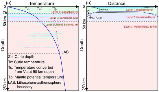
Figure 2. (a) The technical scheme and nomenclature in constructing the temperature structure in this study. (b) A schematic cross-section showing the geometry and spatial relationships of the model layers. Background colors represent different layers.

(1) Within the upper mantle, in Layer 3 (50~250 km depth), the temperature structure is derived directly from the Vs model.

(2) Within transitional Layer 2 (from Curie-point depth, Z_b, to 50 km depth), the temperature is computed by solving the steady-state heat conduction equation, constrained by the Curie temperature at Z_b (T_c) and the Vs-converted temperature at 50 km depth (T_s).

(3) Within magnetic Layer 1 (from the seabed to Z_b), the temperature structure is modeled similarly to Layer 2, but constrained by seafloor temperature and T_c.

In addition, thermal conductivity constitutes a key parameter in the steady-state heat conduction equation. For steps 2 and 3 of the temperature modeling, its value is jointly constrained by the heat flow and the Curie-point depth. Once the 3D temperature structure of the lithosphere is constructed, the thermal lithosphere–asthenosphere boundary (LAB) can be inferred from the intersection with the mantle adiabatic temperature defined by the mantle potential temperature.

2.1. Data Sources

2.1.1. Heat Flow and Curie-Point Depth

A large set of heat flow data in the SCS has been included in the latest Global Heat Flow Database (GHFD) published by the International Heat Flow Commission [47]. Additional heat flow data from the literature is compiled in this study (Table 1; Figure 3a). Heat flow data deviating from the norm may not reflect the true conductive thermal state [9,34], and only heat flow data with values within 30~250 mW/m² is selected for gridding with an interval of 0.25° (Figure 3b). The Curie-point depths (Figure 3c) used in this study are from Li et al. [39], who applied the centroid method to magnetic anomaly data compiled by the Geological Survey of Japan (GSJ) and the Coordinating Committee for Coastal and Offshore Geoscience Programmes in East and Southeast Asia (CCOP). The resulting depths are highly consistent with the tectonic setting of the SCS.

Table 1. Compiled heat flow data in this study.

Data Source	Location
Global Heat Flow Data Assessment Group et al. [47]	Global
Taylor and Hayes [48]	SCS
Rao and Li [49]	North margin
Xiong et al. [50]	South China continent
Nissen et al. [30]	North margin
Shyu et al. [51]	Southwest Taiwan Basin
Mi et al. [52]	North margin
Li et al. [53]	North margin
Tang et al. [36]	North margin
Shi et al. [54]	Qiongdongnan Basin
Shi et al. [55]	Qiongdongnan Basin
Xu et al. [33]	Northwest Sub-basin
Xu et al. [34]	Southwest Sub-basin
IODP 349/367/368 [56,57]	North, south margin; Central Basin
SIO 1	South margin

¹ SIO: Second Institute of Oceanography, Ministry of Natural Resources.

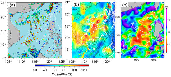
Figure 3. (a) Scatter plot of the observed heat flow in the SCS; (b) Gridded heat flow map of the SCS with earth relief shading; (c) Curie-point depth in the SCS estimated from magnetic data by Li et al. [39]. The white solid line shows the 3000 m isobath.

2.1.2. Vs Model

Chen et al. [42] recently constructed a high-resolution 3D Vs model for the SCS. In this study, three additional Vs models (Table 2) are collected and merged following a three-step procedure designed to ensure consistency and avoid artefacts caused by differing grid resolutions. Direct merging of datasets with variable grid spacing can result in unbalanced spatial sampling, where higher-resolution models dominate the combined output and obscure broader-scale trends present in coarser datasets. This may introduce spurious oscillations or sharp gradients during regridding. To mitigate these issues, we implemented the following steps: (1) Grid unification. All four Vs models are first resampled onto a common three-dimensional grid with uniform intervals of 0.25° in longitude, 0.25° in latitude, and 5 km in depth. (2) Model fusion. At each node of the unified grid, Vs values from the four models are combined by computing a block-mean within a small volumetric window (0.25° × 0.25° × 5 km) centered on the node. This approach reduces spatial aliasing and yields a stable, representative value at each location. (3) Spatial regridding. The fused model is then regridded in three dimensions to enhance internal consistency and smoothness. The final regridding is restricted to the region of interest (108° E~122° E, 5° N~23° N, and 50~250 km in depth, Figure 4), while maintaining the grid interval of 0.25° × 0.25° × 5 km.

Table 2. The Vs model used in this study.

Model	Grid Interval	Range	Data Source
SL2013sv	0.5° × 0.5° × 25 km	X, Y: Global	Schaeffer and Lebedev [58]
		Z: 0~700 km
Chen2021	1° × 1° × 5 km	X: 95° E~125° E	Chen et al. [42]
		Y: 5° S~25° N
		Z: 0~250 km
FWEA18	0.25° × 0.25° × 10 km	X: 90° E~150° E	Tao et al. [43]
		Y: 10° N~60° N
		Z: 0~800 km
SASSY21	0.5° × 0.5° × 5 km	X: 92° E~140° E	Wehner et al. [44]
		Y: 15° S~15° N
		Z: 0~800 km

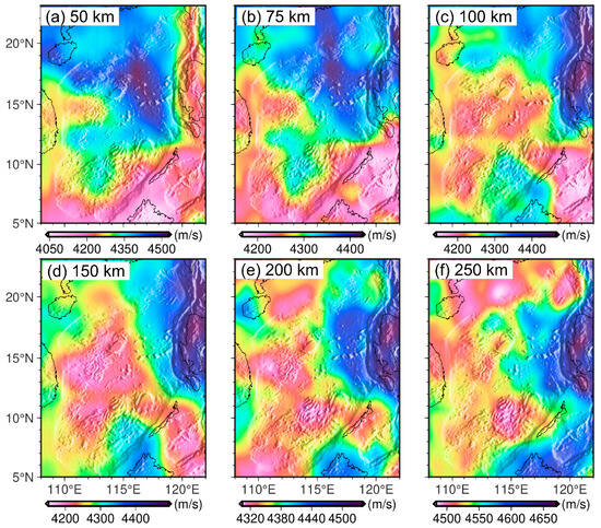
Figure 4. Averaged Vs from four Vs models (SL2013sv, Chen2021, FWEA18 and SASSY21) at different depth slices ((a): at 50 km, (b): at 75 km, (c): at 100 km, (d): at 150 km, (e): at 200 km, (f): at 250 km).

2.2. Methodology

2.2.1. Deriving Upper Mantle Temperature from Vs (50~250 km)

Goes et al. [1] presented a reliable method for converting shear wave velocity to temperature. In their method, the upper mantle is simplified to consist of five key minerals: olivine, orthopyroxene, clinopyroxene, garnet, and spinel. Using a forward model, they calculated the shear modulus and density for a given mineral, temperature, and pressure. To determine the average shear modulus, $⟨\mu ⟩$, and density $⟨\rho ⟩$, for a combination of different minerals, the Voigt–Reuss–Hill averaging scheme was employed. Then, the shear velocity for a given temperature, pressure, and minerals’ combination can be obtained $V_s\left(T,P\right)=\sqrt{⟨\mu ⟩/⟨\rho ⟩}$. With increasing mantle temperature, the anelastic behavior of the mantle material becomes increasingly relevant, and the influence of the anelastic effect on the shear wave velocity was also corrected:

$$Q\left(T,P,\omega \right)=A{\omega }^{a}exp\left(a{\displaystyle \frac{H^{*}+P{V}^{*}}{RT}}\right)$$

(1)

where ω is the frequency, with 0.02 Hz assumed as a representative value for the waves used in the Vs models, and R is the universal gas constant. In accordance with An and Shi [59], the constants A and a are set to 1.48 × 10⁻¹ and 0.15, respectively; the activation energy H* is set to 500 $(\mathrm{k}\mathrm{J}/\mathrm{m}\mathrm{o}\mathrm{l})$ and the activation volume V* is taken as 20 $({\mathrm{c}\mathrm{m}}^3/\mathrm{m}\mathrm{o}\mathrm{l})$. Then the shear wave velocity corrected by the anelastic effect is given by:

$$V_s\left(T,P,\omega \right)=V_s\left(T,P\right)\left[1-{\displaystyle \frac{Q^{-1}\left(T,P,\omega \right)}{2tan\left(\pi a/2\right)}}\right]$$

(2)

The upper mantle composition under different tectonic domains can be roughly classified into three types: on-cratonic, off-cratonic and oceanic [60], and the mineralogical composition for each of these upper mantle types is presented in Table 3. By implementing an inverse calculation, temperature can be derived from the observed shear wave velocity: (1) defining the mineral composition (on-cratonic, off-cratonic or oceanic type) and setting an initial mantle temperature of 0 degree, computing pressure as a function of depth using the earth reference model AK135 [61]; (2) calculating the Vs using the forward modeling procedure and comparing the modeled Vs with the observed one; (3) adjusting the mantle temperature under the Newton’s optimization rule and repeating step (2) until the difference between the modeled and observed Vs is less than 0.1%. Meeßen [62] has incorporated this method in the open-source program VeloDT. For further details on this method, it can be found in [1] and the Supplementary Material.

Table 3. The mineralogical composition for the different types of upper mantle [60].

Type	Olivine	Orthopyroxene	Clinopyroxene	Garnet	Spinel	XFe
On-cratonic	83%	15%	0%	2%	0%	0.086
Off-cratonic	68%	18%	11%	3%	0%	0.1
Oceanic	75%	21%	3.5%	0%	0.5%	0.1

2.2.2. Constraining the Crust and Uppermost Mantle (0~50 km) Temperature Jointly by Heat Flow, Curie-Point Depth, and Vs

The one-dimensional steady heat conduction equation with the temperature-dependent thermal conductivity, $k\left[T\left(z\right)\right]$, is defined as [63]:

$${\displaystyle \frac{d}{dz}}\left(k\left[T\left(z\right)\right]{\displaystyle \frac{dT\left(z\right)}{dz}}\right)=-H_0{e}^{-z/h_r}$$

(3)

where z is the depth, and the surface heat production rate $H_0$ and the drop-off of the heat production $h_r$ are set to $1.37 \mathsf{\mu }\mathrm{W}{·\mathrm{m}}^{-3}$ and $5.0 \mathrm{k}\mathrm{m}$ for the oceanic domain [64]. For the continental domain, these values are set to $2.6 \mathsf{\mu }\mathrm{W}{·\mathrm{m}}^{-3}$ and 10 km [65], respectively. The thermal conductivity varies with temperature and therefore depth [66,67]. Generally, thermal conductivity decreases gradually with increasing temperature until the temperature reaches about 550 °C [67], and then thermal conductivity gradually increases above this temperature [68]. The following temperature-dependent thermal conductivity model is adopted in this study [69]:

$$k\left[T\left(z\right)\right]=\left\{\begin{array}{c}a/\left[1+{\lambda }_{1}T\left(z\right)\right], 0 °\mathrm{C}\le T\left(z\right)\le 550 °\mathrm{C}\\ b/\left[1+{\lambda }_{2}T\left(z\right)\right], T\left(z\right)\ge 550 °\mathrm{C}\end{array}\right.$$

(4)

where ${\lambda }_1=0.001$, ${\lambda }_2=-0.00025$; a and b are the constants that can be estimated from the magnetic layer ($0 °\mathrm{C}\le T\left(z\right)\le 550 °\mathrm{C}, z<Z_b$) by fitting the observed heat flow and the Curie-point depth. Therefore, this model is not only depth-dependent but also generates specific thermal conductivity profiles at different locations due to variable Curie-point depths.

For the magnetic layer ($0 °\mathrm{C}\le T\left(z\right)\le 550 °\mathrm{C}, z<Z_b$), substituting Equation (4) into Equation (3) and integrating Equation (3) twice results in:

$$T\left(z\right)={\displaystyle \frac{1}{{\lambda }_1}}\left(e^{{\displaystyle \frac{{\lambda }_1}{a}}(-h_r^2{H}_0{e}^{-z/h_r}+C_{1}z+C_2)}-1\right)$$

(5)

Assuming that at the Curie-point depth Z_b, the temperature is fixed at the Curie temperature T_c, while the temperature at the seafloor z = Z₀ is T₀, the two constant C₁ and C₂ then can be determined:

$$\left\{\begin{array}{c}{C}_1={\displaystyle \frac{\frac{a}{{\lambda }_1}\mathrm{l}\mathrm{n}\left(\frac{{1+{\lambda }_{1}T}_c}{{1+{\lambda }_{1}T}_0}\right)+h_r^2{H}_0\left(e^{-z_b/h_r}-e^{-z_0/h_r}\right)}{Z_b-Z_0}}\hfill \\ C_2={\displaystyle \frac{Z_b\left[\frac{a}{{\lambda }_1}\mathrm{l}\mathrm{n}\left({1+{\lambda }_{1}T}_0\right)+h_r^2{H}_0{e}^{-z_0/h_r}\right]-Z_0\left[\frac{a}{{\lambda }_1}\mathrm{l}\mathrm{n}\left({1+{\lambda }_{1}T}_c\right)+h_r^2{H}_0{e}^{-z_b/h_r}\right]}{Z_b-Z_0}}\end{array}\right.$$

(6)

From Equation (5) and Fourier’s law of heat conduction, the expression for surface heat flow (q_s) can be derived:

$$q_s=k\left[T\left(z\right)\right]{{\displaystyle \frac{dT\left(z\right)}{dz}}|}_{z=Z_0}=\left({\displaystyle \frac{a}{{\lambda }_1}}\right){\displaystyle \frac{\mathrm{l}\mathrm{n}\left({1+{\lambda }_{1}T}_c\right)-\mathrm{l}\mathrm{n}\left({1+{\lambda }_{1}T}_0\right)}{Z_b-Z_0}}+h_r{H}_0\left[{\displaystyle \frac{h_r}{Z_b-Z_0}}\left(e^{-Z_b/h_r}-e^{-Z_0/h_r}\right)+e^{-Z_0/h_r}\right]$$

(7)

which relates q_s and Z_b. The first term represents background heat flow, and the second term indicates radiogenic heat production in the magnetic layer above the Curie point [65,70]. By fixing $T_0$ and $T_c$ at 5 °C and 550 °C [69], respectively, the unknown constant, a, in the thermal conductivity of the magnetic layer can be estimated through a nonlinear least-squares fit between the $q_s$ and Z_b. Furthermore, the unknown constant, b, in Equation (4) can be determined by ensuring the continuity of thermal conductivity at 550 °C: $b={\displaystyle \frac{a(1+{\lambda }_2{T}_c)}{1+{\lambda }_1{T}_c}}$.

In general, radiogenic heat production in the continental domain is an order of magnitude greater than in the oceanic domain. For each heat flow measurement ($q_s$) point with known coordinates, Z₀ and Z_b are obtained by spatially interpolating bathymetry data (Figure 1) and the regional Curie-depth model (Figure 3c), respectively. Thus, the contributions of radiogenic heat production to heat flow measurements are corrected by subtracting the second term in Equation (7) according to crustal types. The corrected heat flow shows an apparent negative correlation with the thickness of magnetic layer, as expected theoretically (Figure 5). Based on the relationship described in Equation (7), optimal values of a = 4.1 and b = 2.3 for the oceanic domain, as well as a = 3.7 and b = 2.1 for the continental domain, are determined by fitting the corrected heat flow to the thickness of magnetic layer in the least-squares sense.

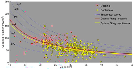
Figure 5. Correlations between corrected heat flow and the thickness of magnetic layer. Observations from the continental margin and central oceanic basin are denoted by yellow and red dots, respectively. Theoretical curves from Equation (7) are shown as blue dashed lines, with corresponding best-fit curves for the oceanic and continental domains plotted as solid red and yellow lines.

Then, by solving Equation (3) numerically, the temperature structure of the crust and uppermost mantle at 0~50 km depth can be constructed. Within the magnetic layer, the following boundary conditions are applied:

$$\left\{\begin{array}{c}T=T_0, Z=Z_0\\ \\ T=T_c, Z=Z_b\end{array}\right.$$

(8)

while the boundary conditions for the temperature calculation from the bottom of the magnetic layer to a depth of 50 km are as follows:

$$\left\{\begin{array}{l}T=T_c, Z=Z_b\\ \\ T=T_s, Z=50 \mathrm{km}\end{array}\right.$$

(9)

where $T_s$ is the Vs-converted temperature at a depth of 50 km.

In contrast to traditional studies where surface heat flow is treated directly as a boundary condition, in this study heat flow is used to constrain the thermal conductivity. It is difficult to estimate the error of the temperature with surface heat flow as boundary conditions when the study area is not stable [59]. Alternatively, both the Curie temperature and the Vs-converted temperature at 50 km depth reflect the current thermal state of the lithosphere and could provide good constraints on both local and regional geotherms.

2.2.3. Determining the LAB

Due to the highly heterogeneous and transitional nature of lithospheric structure, defining the base of the lithosphere presents significant challenges [71]. From a thermal perspective, the base of the lithosphere is often approximated as a constant isotherm. For example, a recent study found that the 1175 ± 50 °C isotherm corresponds well with seismological observations of the LAB [72]. Moreover, several studies have utilized the 1250 °C isotherm to determine the lithospheric base [73,74,75]. A more refined method involves defining the LAB as the point of intersection between the geotherm and the mantle adiabat temperature (T_a) [71] (Figure 2). In this study, T_a is given by: $T_a=T_p+D_a·z$, where a mantle potential temperature (T_p) of 1200 °C [66] and a mantle adiabatic gradient (D_a) of 0.6 °C/km [76] are adopted.

3. Results

3.1. Three-Dimensional Temperature Structure

For the Vs–T conversion, we adopted domain-specific mineralogical compositions: off-cratonic for the continental margins and oceanic for the SCS basin. The Vs-converted temperature structure at 50~250 km depth (Figure 6a) shows that the mantle temperature of the north continental margin, northwest sub-basin and east sub-basin is 100~200 °C lower than that in the surrounding areas at depths of 50~75 km (Figure 6b,c); at depths of 100~150 km, the mantle temperatures of the whole oceanic basins are higher than that of the surrounding areas (Figure 6d,e). Simultaneously, the eastern part of the east sub-basin is cooler than the western part due to the influence of subduction. Down to depths of 200–250 km, the mantle temperature of the east sub-basin is about 180 °C lower than that of the surrounding areas (Figure 6f,g).

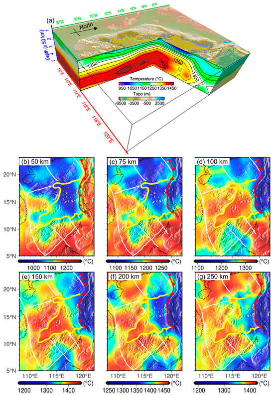
Figure 6. (a) A 3D view of the temperature structure converted from Vs at 50~250 km depth. (b–g) The temperature structure at different horizontal depth slices. The explanation of the boundaries depicted in panels (b–g) can be found in Figure 1.

Then, bounded by the Curie-point depth (Figure 3c) and the Vs-converted temperature at 50 km depth (Figure 6b), the temperature structure at 0~50 km depth (Figure 7a) can be constructed by solving the steady-state heat conduction equation. Overall, the temperature at 0~25 km depth in the central oceanic basin is about 100~200 °C higher than in the surrounding areas (Figure 7b,c). The lithosphere in the north continental margin, the northwest sub-basin, and the east part of the east sub-basin is about 100 °C cooler than the surrounding areas at 40 km depth (Figure 7d).

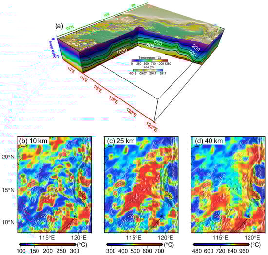
Figure 7. (a) A 3D view of the temperature structure at 0~50 km depth. (b–d) The temperature structure at different horizontal depth slices.

3.2. Uncertainty of the Thermal Model

The surface heat flow can be predicted based on the Fourier’s law of heat conduction (Figure 8a) from our thermal model and compared with the observed data to analyze the uncertainty of our thermal model. The majority of the differences (Figure 8b) between the observed and predicted surface heat flow fall into ±20 mW/m². These differences may be related to both errors in the observed heat flow and uncertainties in our constructed thermal model.

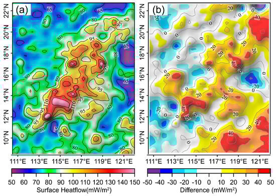
Figure 8. (a) Estimated surface heat flow from our thermal model. (b) Difference between observed (Figure 3b) and estimated surface heat flow. Positive values mean the estimated ones are higher than the observed.

The thermal structure of the upper mantle (50–250 km) is influenced by uncertainties in the Vs–T conversion. These arise from errors in the Vs itself, as well as from uncertainties in mantle composition parameters and anelasticity corrections. In the absence of independent validation, we adopt an assumed temperature uncertainty of 150 °C, consistent with previous studies [1,77].

The uncertainties of the thermal structure in the crust and uppermost mantle (0–50 km) are closely related to the uncertainties in the Curie-point depth. To investigate the influence of the Curie-point depth on the geothermal structure, the geothermal structures at 0~50 km depth are modeled (Figure 9a), where the temperature at 50 km depth is fixed at a temperature close to the average Vs-converted temperature at 50 km depth in the SCS (1100 °C). The results (Figure 9b) show that the corresponding temperature errors caused by per ±10% error in the Curie-point depth are generally not over than ±60 °C. Unlike thermal models based solely on heat flow data, which exhibit rapidly propagating errors with depth [8,60], the integration of heat flow, Curie-point depth, and Vs data yields a model with better-constrained and more manageable uncertainties.

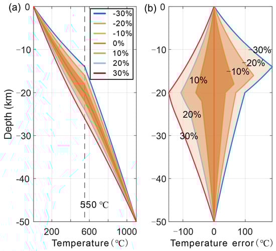
Figure 9. (a) The geothermal structure at 0~50 km depth with different assumed errors in the Curie-point depth. The temperature at 50 km depth is fixed at 1100 °C, which is close to the average Vs-converted temperature at 50 km depth in the SCS; (b) Corresponding geothermal errors caused by different Curie-point depth errors.

4. Discussion

4.1. Moho Temperature and Future Moho Drilling in the SCS

Moho temperature reflects regional variation in both the crustal thickness and lithosphere geotherms [78]. The trade-off between seafloor depth and Moho temperature is one of the most important issues to take into consideration in Moho drilling [6]. Using a refined Moho depth model of Huang et al. [16] (Figure 10a), the Moho temperature in the SCS (Figure 10b) can be extracted from the 3D temperature model.

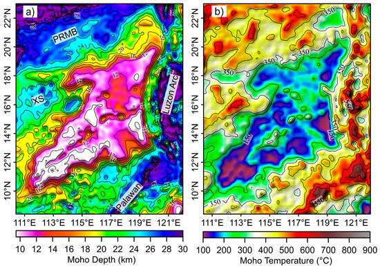
Figure 10. (a) Moho depth in the SCS determined by Huang et al. [16] based on a joint analysis of gravity and seismic data. (b) The Moho temperature estimated in this study. PRMB: Pearl River Mouth Basin; XS: Xisha Islands.

Within the oceanic basin, the Moho temperature is mostly below 250 °C, except for the areas affected by the seamounts. The Moho temperature in the northwest sub-basin varies from 150 to 200 °C; the north flank of the east sub-basin, which is floored by a relatively thick crust, has a Moho temperature varying from 200 to 250 °C overall; the Moho temperature in the south flank of the east sub-basin varies in a range of about 100~250 °C; the southwest sub-basin, floored by a comparatively thinner crust, has a relatively lower Moho temperature, varying mostly from 100~150 °C. Within the continental margin, the Moho temperature is mostly above 350 °C. The highest Moho temperature of over 700 °C is found in the Luzon arc, which is consistent with active volcanism caused by the subduction. In summary, the variation in Moho temperature in the oceanic basin is highly consistent with the variation in crustal thickness, whereas in the continental margin Moho temperature is influenced by both crustal thickness and Curie-point depth.

Ildefonse et al. [6] present some criteria for the possible candidate Moho drilling sites. They emphasized that previous scientific ocean drilling has been limited mostly to temperatures below 200 °C, and that temperatures in excess of ~250 °C may reduce core recovery and increase the risk of hole failure without a substantial re-design of drilling equipment. We integrate various factors, including Moho temperature (mohoT) (Figure 10b), crustal thickness (crsthk) and sediment thickness (sedthk) of Huang et al. [16], and water depth (wd), to evaluate the potential of Moho drilling in the SCS oceanic basin. Each factor is individually scored from 0 to 1 (Figure 11) according to its value by Equation (10). A favorable area, e.g., a thinner crustal thickness, sediment thickness or a lower Moho temperature, or a shallower water depth, will be assigned a higher score. We assign different weights ($w_{crsthk}$, $w_{mohoT}$, $w_{sedthk}$, $w_{wd}$) to each indicator and sum them up (Equation (10)) to obtain the final comprehensive indicator (s) for the potentiality of Moho drilling. In this study, we set the weights of crustal thickness, the Moho surface temperature, sediment thickness, and water depth to 0.6, 0.2, 0.1, and 0.1, respectively, and the corresponding final comprehensive indicator (s) is shown in Figure 12. Using the above methodology, anyone can set the weights according to his/her preferences and come up quickly with an evaluation result. The comprehensive indicator (Figure 12) functions as a preliminary tool to eliminate clearly unsuitable areas, identify zones meeting basic feasibility criteria, and thereby narrows down thousands of potential locations to a shortlist of manageable candidates.

$$\left\{\begin{array}{c}f\left(x\right)={\displaystyle \frac{x_{max}-x}{x_{max}-x_{min}}}\hfill \\ s=w_{crsthk}f\left(crsthk\right)+w_{mohoT}f\left(mohoT\right)+w_{sedthk}f\left(sedthk\right)+w_{wd}f\left(wd\right)\end{array}\right.$$

(10)

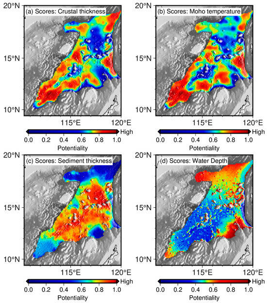
Figure 11. The potentiality of Moho Drilling in the SCS oceanic basin when it is only assessed by crustal thickness (a), Moho temperature (b), sediment thickness (c), or water depth (d), respectively. The closer to 1 in the indicator, the higher the potentiality.

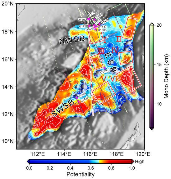
Figure 12. A comprehensive indicator reflecting the potentiality of Moho drilling. The closer to 1 in the value, the higher is the potentiality. The dots show the Moho depths determined from seismic data [16]. The red dashed line shows the Zhongnan Fault. The magenta stars indicate the drill sites of IODP Expeditions 349 and 367/368. The red boxes mark six areas in the east sub-basin with high potential for Moho drilling, where zone V is originally proposed by Qin et al. [79]. ESB: east sub-basin; NWSB: northwest sub-basin; SWSB: southwest sub-basin.

Both gravity inversion [16] and seismic surveys [80,81] show that the southwest sub-basin has a relatively thin crust, formed with a slow spreading rate [28,82]. Although the potential for Moho surface drilling is relatively high in most areas of the southwest sub-basin (Figure 12), except for areas with seamounts near the residual mid-ocean ridges, the Moho reflection is weak in the southwest sub-basin [79,80], which does not meet the requirement for successful Moho drilling [6]. A better-imaged Moho is required in the southwest sub-basin for Moho drilling.

In the northwest sub-basin, the potentiality of Moho drilling is relatively high in its central area, and there are no obvious high Vp anomalies in the crust [83]. The Moho temperature in this region is about 130~170 °C, but the sediment thickness is relatively thick, varying from 1400 to 1800 m.

In the east sub-basin, we identify six areas with relatively high potentiality of Moho drilling (Figure 12; Table 4) and our Zone V coincides with that originally proposed by Qin et al. [79] based on a large volume of deep reflection seismic data. The Moho temperatures in these regions range from ~120 to 190 °C. The gravity inversion results show that the crustal thicknesses in Zones II and VI are mostly less than 5 km, and the OBS survey showed that the crustal thickness in Zone II can be as thin as about 4.0 km [84]. Clear and strong Moho reflections have only been mapped in Zones I and V [79,85], and there are few public deep reflection seismic profiles in the rest of zones; the Moho reflection characteristics in these zones require further investigation.

Table 4. The principal characteristics of the identified areas with relatively high potential for Moho drilling in the east sub-basin of the SCS.

Zones	I	II	III	IV	V	VI
FSR (km/Myr)	40~55	53~66	45~50	45~50	45~56	45~50
τ (Ma)	27.5~30	24.5~28	18~22	18~22	21~26	16~23
Moho-T (°C)	170~190	120~180	135~170	130~180	120~170	~120
WD (m)	3800~4050	3900~4200	3800~4200	3700~4250	4000~4300	4000~4500
Thksed (m)	1270~1850	1250~1950	500~700	500~1200	420~820	500~1100
Thkcrust (km)	5.0~6.5	4.0~5.3	5.1~6.0	5.4~6.3	5.3~7.5	3.0~5.1
L (km)	10.3~11.7	9.4~11.7	10.0~11.2	10.0~10.8	9.6~12.3	7.8~10.0

FSR: Full-Spreading Rate; τ: Crustal Age; Moho-T: Moho Temperature; WD: Water Depth; Thksed: Sediment Thickness; Thkcrust: Crystal Crust Thickness; L: Total Length to the Moho. Full-spreading rate and crustal age are adopted from Seton et al. [86]. Water depth is extracted from GEBCO_2020 [87]. Sediment thickness, crustal thickness and Moho depth are from Huang et al. [16].

Deep reflection seismic profiles crossing Zone I show shallow and clear Moho reflections, and the oceanic crust may be as thin as ~1.3–1.5 s in two-way travel time (~4~4.5 km, converted with a constant Vp of 6.0 km/s for oceanic crust) [85]. In addition, Hole U1503 from IODP Expedition 367/368 is located near the north edge of Zone I, and it remains cased and open for possible future occupation [57]. These factors provide favorable conditions for further determination of the specific potential Moho drilling sites in Zone I in the future.

4.2. Thermal State of the Lithosphere and Its Relation to Tectonic Features

Figure 13 shows the lithosphere–asthenosphere boundary (LAB) derived from our 3D thermal model. Limited by the low resolution of the S-wave model used in previous studies, the lithosphere thickness determined in previous studies exhibited almost a uniform thickness in the SCS [3,21,76]. Our thermal LAB results are based on the S-wave model merged from four high-resolution models and show more local variations in the SCS (Figure 13).

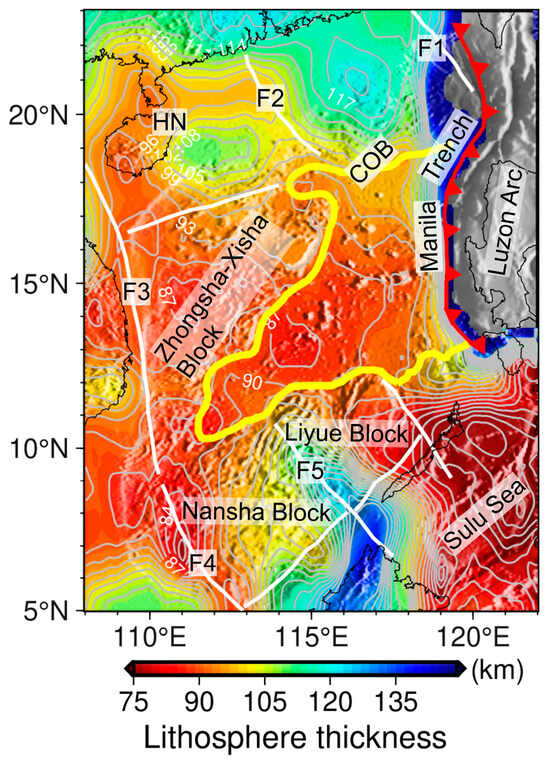
Figure 13. The thickness of the thermal lithosphere in the SCS. The yellow line indicates the continental–ocean boundary (COB) [23,24,25]. The red line marks the Manila Trench. The white lines mark the main faults in the continental margin from Wu and Wen [26]. F1: Shantou–Balintang Fault; F2: Yangjiang–Yitong Fault Zone; F3: West Continental Margin Fault; F4: Tinjar Fault; F5: Balabac Fault; HN: Hainan.

4.2.1. Continental Margin

The thermal lithosphere thickness to the east of the Yangjiang–Yitong Fault Zone (F2) in the northern continental margin is relatively thicker, ranging from 105 to 120 km, than to the west of F2, varying from 90 to 108 km. The thinnest thermal lithosphere in this region is found in northeast Hainan, where there may be a mantle plume [88]. Our temperature structure results also show relatively hot lithosphere beneath the Hainan hotspot (Figure 6a–e).

Throughout the northwest continental margin (Zhongsha–Xisha Block), the thermal lithosphere is relatively thin, typically varying from 87 to 96 km, and a notable thinning is observed around the West Continental Margin Fault (F3), which is the extension of the deep lithospheric Red River Fault [26,89]. The lithosphere around F3 may have undergone severe deformation and destruction during the extrusion of the Indochina block due to the collision of the Indian and Eurasian plates, and accompanied by the upwelling of deep mantle material, resulting in a relatively thin thermal lithosphere along the fault.

In the southern continental margin, the Nansha Block and Liyue Block exhibit different thermal states bounded by the Balabac Fault (F5). The thermal lithosphere in the Nansha Block is generally thicker than that in the Liyue Block. Except in the area near Tinjar Fault (F4), Nansha Block has a thermal lithosphere thickness of about 100 km, which is consistent with the result from Dong et al. [46] (Table 5). The thermal lithosphere thickness in the Liyue Block is about 85 km. F4 and F5 show sharp contrast in thermal lithosphere thickness; F4 is an active trans-lithospheric fault [90,91], along which massive magmatic intrusions have been found [92], whereas the activity of F5 is relatively weak after Early Miocene [91]. In summary, our thermal lithosphere thickness in the continental margin of the SCS are broadly consistent with the tectonic settings.

Table 5. The lithospheric thickness in the SCS from different studies.

Data	Central Basin (km)	Margin (km)	Reference
Heat flow	-	86~96 (N)	Shi et al. [35]
Vp	80~100	60~80	Yao and Wan [89]
Vs	70~80	70~80	Tang and Zheng [21]
T from Vs	70~80	70~80	Yu et al. [3]
Gravity	60~90	90~120	Chen et al. [93]
T from Vs	-	80~125(S)	Dong et al. [46]
Heat flow	35~55	35~55 (N) 80~100 (S)	Wang et al. [37]
Topography	46~60 (NW)	-	Wang et al. [14]
T from Vs	85~96	96~120 (N) 81~125 (S)	This study

4.2.2. Oceanic Basin

The lithosphere thickness in the oceanic basin of the SCS varies from 85 to 96 km, which is comparable to the result of Yao and Wan [89] based on P-wave tomography (Table 5), and Chen et al. [93] based on gravity inversion, but relatively higher than the results based on S-wave tomography [21] and its derivative of thermal structure [3]. Overall, the lithosphere in the oceanic basin of SCS determined in this study (85–100 km) and previous studies (60–100 km) [3,21,89,93] (Table 5) is thicker than those predicted by the theoretical models (e.g., 50–60 km predicted by the half-space cooling model in the SCS). Yao and Wan [89] argued that the new oceanic crust combined with the remained ultramafic rocks with high seismic velocities at about 50~80 km depth to thicken the new SCS oceanic lithosphere. Furthermore, as seafloor spreading in the South China Sea ceased after 15 Ma [28], its oceanic lithosphere has cooled more rapidly than the lithosphere of comparable age at active ridges, due to the absent ongoing mantle heat supply.

In addition, An et al. [10] found that the cooling or thermal structure of oceanic lithosphere beneath the Antarctic Plate is dependent on the spreading rate of the ridge. To investigate the relationship between cooling and spreading rate globally, the theoretical oceanic lithosphere thickness proposed by Parker and Oldenburg [94] is subtracted from the observed ones [20] (Figure 14a). Their differences plotted against with the full spreading rate (Figure 14b) mainly fall into −10~40 km, and only the differences in the ultra-slow (<20 km/Myr) and slow (20~50 km/Myr) spreading rate are anomalously high, over 100 km (Figure 14b). The relationships between oceanic lithosphere thickness and age are scattered and deviate from the theoretical prediction when the full spreading rate is below 50 km/Myr (ultra-slow and slow) (Figure 14c), whereas the points are more concentrated and closer to the theoretical predictions when the full spreading rate is above 50 km/Myr (intermediate, fast and superfast) (Figure 14d), further suggesting that the oceanic lithosphere generated with the ultra-slow or slow spreading rate is more likely to be thicker. Given the slow spreading history of the SCS (full spreading rates: 26–46 mm/yr, southwest sub-basin [82]; mostly 20–50 mm/yr, east sub-basin [28]), the observed thick oceanic lithosphere likely results from the combined effect of the residual high-velocity ultramafic layer and the slow spreading rate.

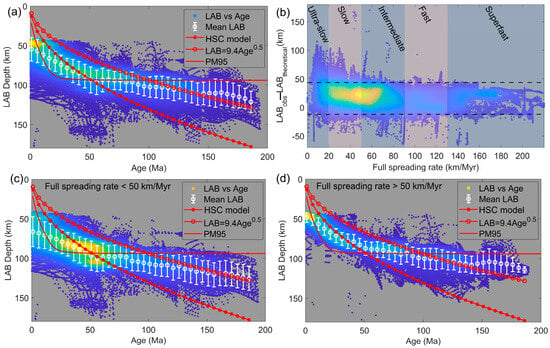
Figure 14. Global LAB depth versus crustal age and spreading rate. Colors indicate the degree of scatter aggregation, with yellower hues representing higher clustering. (a) LAB depth versus seafloor crustal age. White circles (error bars) show 5 Myr averaged values (standard deviations). Theoretical LAB depths are shown for the half-space cooling [95], Parker and Oldenburg [94], and plate cooling (Plate thickness: 95 km) models [96]. (b) Difference between observed [20] and theoretical [95] LAB depths versus full spreading rate. (c,d) Same as (a) for ultra-slow/slow (c) and intermediate-to-superfast (d) spreading regimes. (Data: LAB from Hoggard et al. [20] based on CAM2016 Vs model; crustal age from Seton et al. [86]).

5. Conclusions

In this study, we have developed an integrated approach to construct a 3D thermal model of the SCS lithosphere using heat flow, Curie-point depth, and Vs data. This methodology could reduce the uncertainties inherent in models relying on a single data type. Our key findings are as follows:

1. Our model reveals that the Moho temperature is below 250 °C in the most part of the SCS oceanic basin, but generally above 350 °C in the continental margins.

2. A comprehensive assessment for potential future Moho drilling sites was conducted by synthesizing key factors, including Moho temperature, crustal thickness, sediment thickness, and water depth. Six promising zones in the east sub-basin are identified, while weak Moho reflections currently hinder site selection in the southwest sub-basin despite favorable thermal conditions.

3. The derived thermal LAB correlates well with tectonic settings in the continental margins. Notably, the oceanic lithosphere is anomalously thick compared to theoretical predictions.

4. Global analysis links the anomalously thick oceanic lithosphere to ultra-slow and slow-spreading ridges. Thus, the lithospheric thickening in the SCS oceanic basin was likely jointly caused by a residual high-velocity ultramafic layer and the slow spreading rate during its formation.

Our integrated 3D thermal model refines the present-day thermal structure of the SCS, thereby providing critical constraints for reinterpretations of its tectonic evolution. The methodology we present paves the way for lithospheric thermal studies in other complex marginal basins globally.

References

- Goes, S.; Govers, R.; Vacher, P. Shallow mantle temperatures under Europe from P and S wave tomography. J. Geophys. Res. Solid Earth 2000, 105, 11153–11169. [Google Scholar] [CrossRef]
- Artemieva, I.M. Global 1°×1° thermal model TC1 for the continental lithosphere: Implications for lithosphere secular evolution. Tectonophysics 2006, 416, 245–277. [Google Scholar] [CrossRef]
- Yu, C.; Shi, X.; Yang, X.; Zhao, J.; Chen, M.; Tang, Q. Deep thermal structure of Southeast Asia constrained by S-velocity data. Mar. Geophys. Res. 2017, 38, 341–355. [Google Scholar] [CrossRef]
- Niu, Y. Do we really need to drill through the intact ocean crust? Geosci. Front. 2025, 16, 101954. [Google Scholar] [CrossRef]
- Sun, Z.; Xu, Y.; Deng, Y. The Moho is in reach of ocean drilling with the Meng Xiang. Nat. Geosci. 2025, 18, 275–276. [Google Scholar] [CrossRef]
- Ildefonse, B.; Abe, N.; Blackman, D.K.; Canales, J.P.; Isozaki, Y.; Kodaira, S.; Myers, G.; Nakamura, K.; Nedimovic, M.; Skinner, A.C.; et al. The MoHole: A Crustal Journey and Mantle Quest, Workshop in Kanazawa, Japan, 3–5 June 2010. Sci. Dril. 2010, 10, 56–63. [Google Scholar] [CrossRef]
- Tanaka, A.; Ishikawa, Y. Temperature distribution and focal depth in the crust of the northeastern Japan. Earth Planets Space 2002, 54, 1109–1113. [Google Scholar] [CrossRef]
- Artemieva, I.M.; Mooney, W.D. Thermal thickness and evolution of Precambrian lithosphere: A global study. J. Geophys. Res. Solid Earth 2001, 106, 16387–16414. [Google Scholar] [CrossRef]
- Lucazeau, F. Analysis and Mapping of an Updated Terrestrial Heat Flow Data Set. Geochem. Geophys. Geosyst. 2019, 20, 4001–4024. [Google Scholar] [CrossRef]
- An, M.; Wiens, D.A.; Zhao, Y.; Feng, M.; Nyblade, A.A.; Kanao, M.; Li, Y.; Maggi, A.; Lévêque, J.-J. Temperature, lithosphere-asthenosphere boundary, and heat flux beneath the Antarctic Plate inferred from seismic velocities. J. Geophys. Res. Solid Earth 2015, 120, 359–383. [Google Scholar] [CrossRef]
- Li, C.-F. An integrated geodynamic model of the Nankai subduction zone and neighboring regions from geophysical inversion and modeling. J. Geodyn. 2011, 51, 64–80. [Google Scholar] [CrossRef]
- Afonso, J.C.; Fernàndez, M.; Ranalli, G.; Griffin, W.L.; Connolly, J.A.D. Integrated geophysical-petrological modeling of the lithosphere and sublithospheric upper mantle: Methodology and applications. Geochem. Geophys. Geosyst. 2008, 9, Q05008. [Google Scholar] [CrossRef]
- Artemieva, I.M. Lithosphere structure in Europe from thermal isostasy. Earth-Sci. Rev. 2019, 188, 454–468. [Google Scholar] [CrossRef]
- Wang, X.; Huang, H.; Xu, H.; Ren, Z.; Zhang, J.; Zhao, Z. The deep thermal structure of the lithosphere in the northwestern South China Sea and its control on the shallow tectonics. Sci. China Earth Sci. 2021, 64, 962–976. [Google Scholar] [CrossRef]
- Xia, B.; Artemieva, I.M.; Thybo, H.; Klemperer, S.L. Strong variability in the thermal structure of Tibetan Lithosphere. J. Geophys. Res. Solid Earth 2023, 128, e2022JB026213. [Google Scholar] [CrossRef]
- Huang, L.; Wen, Y.; Li, C.-F.; Peng, X.; Lu, Z.; Xu, L.; Yao, Y. A refined Moho depth model from a joint analysis of gravity and seismic data of the South China Sea basin and its tectonic implications. Phys. Earth Planet. Inter. 2023, 334, 106966. [Google Scholar] [CrossRef]
- Nolet, G.; Zielhuis, A. Low S velocities under the Tornquist-Teisseyre zone: Evidence for water injection into the transition zone by subduction. J. Geophys. Res. Solid Earth 1994, 99, 15813–15820. [Google Scholar] [CrossRef]
- Sobolev, S.V.; Zeyen, H.; Stoll, G.; Werling, F.; Altherr, R.; Fuchs, K. Upper mantle temperatures from teleseismic tomography of French Massif Central including effects of composition, mineral reactions, anharmonicity, anelasticity and partial melt. Earth Planet. Sci. Lett. 1996, 139, 147–163. [Google Scholar] [CrossRef]
- Ritzwoller, M.H.; Shapiro, N.M.; Zhong, S.-J. Cooling history of the Pacific lithosphere. Earth Planet. Sci. Lett. 2004, 226, 69–84. [Google Scholar] [CrossRef]
- Hoggard, M.J.; Czarnota, K.; Richards, F.D.; Huston, D.L.; Jaques, A.L.; Ghelichkhan, S. Global distribution of sediment-hosted metals controlled by craton edge stability. Nat. Geosci. 2020, 13, 504–510. [Google Scholar] [CrossRef]
- Tang, Q.; Zheng, C. Crust and upper mantle structure and its tectonic implications in the South China Sea and adjacent regions. J. Asian Earth Sci. 2013, 62, 510–525. [Google Scholar] [CrossRef]
- Gao, G.; Lu, Q.; Wang, J.; Kang, G. Constraining crustal thickness and lithospheric thermal state beneath the northeastern Tibetan Plateau and adjacent regions from gravity, aeromagnetic, and heat flow data. J. Asian Earth Sci. 2021, 212, 104743. [Google Scholar] [CrossRef]
- Song, T.; Li, C.-F.; Wu, S.; Yao, Y.; Gao, J. Extensional styles of the conjugate rifted margins of the South China Sea. J. Asian Earth Sci. 2019, 177, 117–128. [Google Scholar] [CrossRef]
- Wen, Y.; Li, C.-F.; Wang, L.; Liu, Y.; Peng, X.; Yao, Z.; Yao, Y. The onset of seafloor spreading at the northeastern continent-ocean boundary of the South China Sea. Mar. Pet. Geol. 2021, 133, 105255. [Google Scholar] [CrossRef]
- Nirrengarten, M.; Mohn, G.; Kusznir, N.J.; Sapin, F.; Despinois, F.; Pubellier, M.; Chang, S.P.; Larsen, H.C.; Ringenbach, J.C. Extension modes and breakup processes of the southeast China-Northwest Palawan conjugate rifted margins. Mar. Pet. Geol. 2020, 113, 104123. [Google Scholar] [CrossRef]
- Wu, Z.; Wen, Z. Map Series of Marine Geology of China Seas; Science Press: Beijing, China, 2019. (In Chinese) [Google Scholar]
- Li, C.-F.; Li, J.; Ding, W.; Franke, D.; Yao, Y.; Shi, H.; Pang, X.; Cao, Y.; Lin, J.; Kulhanek, D.K.; et al. Seismic stratigraphy of the central South China Sea basin and implications for neotectonics. J. Geophys. Res. Solid Earth 2015, 120, 1377–1399. [Google Scholar] [CrossRef]
- Li, C.-F.; Xu, X.; Lin, J.; Sun, Z.; Zhu, J.; Yao, Y.; Zhao, X.; Liu, Q.; Kulhanek, D.K.; Wang, J.; et al. Ages and magnetic structures of the South China Sea constrained by deep tow magnetic surveys and IODP Expedition 349. Geochem. Geophys. Geosyst. 2014, 15, 4958–4983. [Google Scholar] [CrossRef]
- Peng, X.; Li, C.-F. Along-strike break-up variations of the continent–ocean transition zone in the northern South China Sea. J. Geol. Soc. 2024, 181, jgs2023-134. [Google Scholar] [CrossRef]
- Nissen, S.S.; Hayes, D.E.; Bochu, Y.; Zeng, W.; Chen, Y.; Nu, X. Gravity, heat flow, and seismic constraints on the processes of crustal extension: Northern margin of the South China Sea. J. Geophys. Res. Solid Earth 1995, 100, 22447–22483. [Google Scholar] [CrossRef]
- He, L.; Wang, K.; Xiong, L.; Wang, J. Heat flow and thermal history of the South China Sea. Phys. Earth Planet. Inter. 2001, 126, 211–220. [Google Scholar] [CrossRef]
- Shi, X.; Qiu, X.; Xia, K.; Zhou, D. Characteristics of surface heat flow in the South China Sea. J. Asian Earth Sci. 2003, 22, 265–277. [Google Scholar] [CrossRef]
- Xu, X.; Wang, X.; Peng, D.; Yao, Y.; Yao, B.; Wan, Z. Characteristics and Research of Heat Flow in the Northwest Sub-Basin and Its Adjacent Areas of the South China Sea. Earth Sci. 2018, 43, 3391–3398. (In Chinese) [Google Scholar]
- Xu, X.; Yao, Y.; Peng, D.; Yao, B. The characteristics and analysis of heat flow in the Southwest sub-basin of South China Sea. Chin. J. Geophys. 2018, 61, 2915–2925. (In Chinese) [Google Scholar]
- Shi, X.; Zhou, D.; Zhang, Y. Lithospheric thermal-rheological structures of the continental margin in the northern South China Sea. Chin. Sci. Bull. 2000, 45, 1660–1665. (In Chinese) [Google Scholar] [CrossRef]
- Tang, X.; Hu, S.; Zhang, G.; Yang, S.; Sheng, H.; Rao, S.; Li, W. Characteristic of surface heat flow in the Pearl River Mouth Basin and its relationship with thermal lithosphere thickness. Chin. J. Geophys. 2014, 557, 1857–1867. (In Chinese) [Google Scholar]
- Wang, X.; Wang, K.; Zhao, Z.; Xu, H.; Zhao, J.; Ren, Z.; Zhang, J. Three-dimensional thermal structure of the lithosphere and its relationship to surface structure in the South China Sea. Chin. J. Geophys. 2021, 64, 4105–4116. (In Chinese) [Google Scholar] [CrossRef]
- Zhu, W.; Liu, S. Heat flow and thermal structure of the South China Sea. Earth-Sci. Rev. 2025, 261, 105028. [Google Scholar] [CrossRef]
- Li, C.-F.; Shi, X.; Zhou, Z.; Li, J.; Geng, J.; Chen, B. Depths to the magnetic layer bottom in the South China Sea area and their tectonic implications. Geophys. J. Int. 2010, 182, 1229–1247. [Google Scholar] [CrossRef]
- Wu, Z.; Gao, J.Y.; Zhao, L.; Zhang, T.; Yang, C.; Wang, J. Characteristic of Magnetic Anomalies and Curie Point Depth at Northern Continental Margin of the South China Sea. Earth Sci. 2010, 35, 1060–1068. (In Chinese) [Google Scholar] [CrossRef]
- Ren, Z.; Shi, X.; Wang, X.; Zhao, P.; Shen, Y. Deep thermal state in the Nansha Trough of South China Sea and its tectonic implications. J. Trop. Oceanogr. 2021, 40, 98–109. (In Chinese) [Google Scholar] [CrossRef]
- Chen, H.; Li, Z.; Luo, Z.; Ojo, A.O.; Xie, J.; Bao, F.; Wang, L.; Tu, G. Crust and Upper Mantle Structure of the South China Sea and Adjacent Areas from the Joint Inversion of Ambient Noise and Earthquake Surface Wave Dispersions. Geochem. Geophys. Geosyst. 2021, 22, e2020GC009356. [Google Scholar] [CrossRef]
- Tao, K.; Grand, S.P.; Niu, F. Seismic Structure of the Upper Mantle Beneath Eastern Asia from Full Waveform Seismic Tomography. Geochem. Geophys. Geosyst. 2018, 19, 2732–2763. [Google Scholar] [CrossRef]
- Wehner, D.; Blom, N.; Rawlinson, N.; Daryono; Böhm, C.; Miller, M.S.; Supendi, P.; Widiyantoro, S. SASSY21: A 3-D Seismic Structural Model of the Lithosphere and Underlying Mantle Beneath Southeast Asia from Multi-Scale Adjoint Waveform Tomography. J. Geophys. Res. Solid Earth 2022, 127, e2021JB022930. [Google Scholar] [CrossRef]
- Meeßen, C.; Sippel, J.; Scheck-Wenderoth, M.; Heine, C.; Strecker, M.R. Crustal Structure of the Andean Foreland in Northern Argentina: Results from Data-Integrative Three-Dimensional Density Modeling. J. Geophys. Res. Solid Earth 2018, 123, 1875–1903. [Google Scholar] [CrossRef]
- Dong, M.; Zhang, J.; Wu, S.-G.; Wang, B.-Y.; Ai, Y.-F. Cooling of the lithosphere beneath the Nansha Block, South China Sea. J. Asian Earth Sci. 2019, 171, 169–177. [Google Scholar] [CrossRef]
- Global Heat Flow Data Assessment Group; Fuchs, S.; Neumann, F.; Norden, B.; Beardsmore, G.; Chiozzi, P.; Colgan, W.; Anguiano Dominguez, A.P.; Duque, M.R.A.; Ojeda Espinoza, O.M.; et al. The Global Heat Flow Database: Update 2023. V. 1. GFZ Data Serv. 2023. Available online: https://dataservices.gfz-potsdam.de/panmetaworks/showshort.php?id=38ab063c-9e6d-11ed-95b8-f851ad6d1e4b (accessed on 5 March 2024).
- Taylor, B.; Hayes, D.E. Origin and History of the South China Sea Basin. In The Tectonic and Geologic Evolution of Southeast Asian Seas and Islands: Part 2; Hayes, D.E., Ed.; Geophysical Monograph Series; American Geophysical Union: Washington, DC, USA, 1983; pp. 23–56. [Google Scholar]
- Rao, C.; Li, P. Study of Heat Flow in Pearl River Mouth Basin. China Offshore Oil Gas (Geol.) 1991, 5, 7–18. (In Chinese) [Google Scholar]
- Xiong, L.; Hu, S.; Wang, J. Terrestrial heat flow values in southeastern China. Chin. J. Geophys. 1993, 36, 784–790. (In Chinese) [Google Scholar]
- Shyu, C.-T.; Hsu, S.-K.; Liu, C.-S. Heat Flows off Southwest Taiwan: Measurements over Mud Diapirs and Estimated from Bottom Simulating Reflectors. Terr. Atmos. Ocean. Sci. 1998, 9, 795–812. [Google Scholar] [CrossRef]
- Mi, L.; Yuan, Y.; Zhang, G.; Hu, S.; He, L.; Yang, S. Characteristics and genesis of geothermal field in deep-water area of the northern South China Sea. Acta Petrolei Sinica 2009, 30, 27–32. (In Chinese) [Google Scholar]
- Li, Y.; Luo, X.; Xu, X.; Yang, X.; Shi, X. Seafloor in-situ heat flow measurements in the deep-water area of the northern slope, South China Sea. Chin. J. Geophys. 2010, 53, 2161–2170. (In Chinese) [Google Scholar]
- Shi, X.; Wang, Z.; Jiang, H.; Sun, Z.; Sun, Z.; Yang, J.; Yu, C.; Yang, X. Vertical variations of geothermal parameters in rifted basins and heat flow distribution features of the Qiongdongnan Basin. Chin. J. Geophys. 2015, 58, 939–953. (In Chinese) [Google Scholar]
- Shi, X.; Jiang, H.; Yang, J.; Yang, X.; Xu, H. Models of the rapid post-rift subsidence in the eastern Qiongdongnan Basin, South China Sea: Implications for the development of the deep thermal anomaly. Basin Res. 2017, 29, 340–362. [Google Scholar] [CrossRef]
- Li, C.F.; Lin, J.; Kulhanek, D.K.; Williams, T.; Bao, R.; Briais, A.; Brown, E.A.; Chen, Y.; Clift, P.D.; Colwell, F.S.; et al. Proceedings of the International Ocean Discovery Program, 349: South China Sea Tectonics; International Ocean Discovery Program: College Station, TX, USA, 2015. [Google Scholar]
- Sun, Z.; Jian, Z.; Stock, J.M.; Larsen, H.C.; Klaus, A.; Alvarez Zarikian, C.A.; Boaga, J.; Bowden, S.A.; Briais, A.; Chen, Y.; et al. South China Sea Rifted Margin. Proceedings of the International Ocean Discovery Program; International Ocean Discovery Program: College Station, TX, USA, 2018; Volume 367/368. [Google Scholar]
- Schaeffer, A.J.; Lebedev, S. Global shear speed structure of the upper mantle and transition zone. Geophys. J. Int. 2013, 194, 417–449. [Google Scholar] [CrossRef]
- An, M.; Shi, Y. Three-dimensional thermal structure of the Chinese continental crust and upper mantle. Sci. China Ser. D Earth Sci. 2007, 50, 1441–1451. [Google Scholar] [CrossRef]
- Shapiro, N.M.; Ritzwoller, M.H. Thermodynamic constraints on seismic inversions. Geophys. J. Int. 2004, 157, 1175–1188. [Google Scholar] [CrossRef]
- Kennett, B.L.N.; Engdahl, E.R.; Buland, R. Constraints on seismic velocities in the Earth from traveltimes. Geophys. J. Int. 1995, 122, 108–124. [Google Scholar] [CrossRef]
- Meeßen, C. cmeessen/VeloDT: VeloDT v1.2. Zenodo. 2020. Available online: https://zenodo.org/records/3895784 (accessed on 1 June 2023).
- Turcotte, D.; Schubert, J. Geodynamics, 2nd ed.; Cambridge University Press: Cambridge, UK, 2002. [Google Scholar]
- Li, C.-F.; Wang, J.; Lin, J.; Wang, T. Thermal evolution of the North Atlantic lithosphere: New constraints from magnetic anomaly inversion with a fractal magnetization model. Geochem. Geophys. Geosyst. 2013, 14, 5078–5105. [Google Scholar] [CrossRef]
- Lu, Y.; Li, C.-F.; Wang, J.; Wan, X. Arctic geothermal structures inferred from Curie-point depths and their geodynamic implications. Tectonophysics 2022, 822, 229158. [Google Scholar] [CrossRef]
- Zang, S.; Liu, Y.; Ning, J. Thermal structure of North China lithosphere. Chin. J. Geophys. 2002, 45, 56–66. (In Chinese) [Google Scholar]
- Whittington, A.G.; Hofmeister, A.M.; Nabelek, P.I. Temperature-dependent thermal diffusivity of the Earth’s crust and implications for magmatism. Nature 2009, 458, 319–321. [Google Scholar] [CrossRef]
- Jaupart, C.; Mareschal, J.C.; Guillou-Frottier, L.; Davaille, A. Heat flow and thickness of the lithosphere in the Canadian Shield. J. Geophys. Res. Solid Earth 1998, 103, 15269–15286. [Google Scholar] [CrossRef]
- Li, C.-F.; Wang, J.; Zhou, Z.; Geng, J.; Chen, B.; Yang, F.; Wu, J.; Yu, P.; Zhang, X.; Zhang, S. 3D geophysical characterization of the Sulu–Dabie orogen and its environs. Phys. Earth Planet. Inter. 2012, 192–193, 35–53. [Google Scholar] [CrossRef]
- Andrés, J.; Marzán, I.; Ayarza, P.; Martí, D.; Palomeras, I.; Torné, M.; Campbell, S.; Carbonell, R. Curie Point Depth of the Iberian Peninsula and Surrounding Margins. A Thermal and Tectonic Perspective of its Evolution. J. Geophys. Res. 2018, 123, 2049–2068. [Google Scholar] [CrossRef]
- Artemieva, I.M. The Lithosphere: An Interdisciplinary Approach; Cambridge University Press: Cambridge, UK, 2011. [Google Scholar]
- Richards, F.D.; Hoggard, M.J.; Cowton, L.R.; White, N.J. Reassessing the Thermal Structure of Oceanic Lithosphere with Revised Global Inventories of Basement Depths and Heat Flow Measurements. J. Geophys. Res. Solid Earth 2018, 123, 9136–9161. [Google Scholar] [CrossRef]
- Fullea, J.; Afonso, J.C.; Connolly, J.A.D.; Fernàndez, M.; García-Castellanos, D.; Zeyen, H. LitMod3D: An interactive 3-D software to model the thermal, compositional, density, seismological, and rheological structure of the lithosphere and sublithospheric upper mantle. Geochem. Geophys. Geosyst. 2009, 10, Q08019. [Google Scholar] [CrossRef]
- Afonso, J.C.; Ben-Mansour, W.; O’Reilly, S.Y.; Griffin, W.L.; Salajeghegh, F.; Foley, S.; Begg, G.; Selway, K.; Macdonald, A.; Januszczak, N.; et al. Thermochemical structure and evolution of cratonic lithosphere in central and southern Africa. Nat. Geosci. 2022, 15, 405–410. [Google Scholar] [CrossRef]
- Yang, X.; Li, Y.; Afonso, J.C.; Yang, Y.; Zhang, A. Thermochemical State of the Upper Mantle Beneath South China from Multi--Observable Probabilistic Inversion. J. Geophys. Res. Solid Earth 2021, 126, e2020JB021114. [Google Scholar] [CrossRef]
- Priestley, K.; McKenzie, D.; Ho, T. A Lithosphere–Asthenosphere Boundary—A Global Model Derived from Multimode Surface-Wave Tomography and Petrology. In Lithospheric Discontinuities; Yuan, H., Romanowicz, B., Eds.; Geophysical Monograph Series; American Geophysical Union: Washington, DC, USA, 2018; pp. 111–123. [Google Scholar]
- An, M.; Shi, Y. Lithospheric thickness of the Chinese continent. Phys. Earth Planet. Inter. 2006, 159, 257–266. [Google Scholar] [CrossRef]
- Artemieva, I.M.; Shulgin, A. Geodynamics of Anatolia: Lithosphere Thermal Structure and Thickness. Tectonics 2019, 38, 4465–4487. [Google Scholar] [CrossRef]
- Qin, X.; Zhang, B.; Zhao, B.; Lu, Y.; Chen, X.; Wang, L.; Xu, Z.; Zhang, R.; Geng, M.; Yang, Z.; et al. Distribution characteristics of Mohorovicic discontinuity in the South China Sea basin and suggestions for drilling preparation area. Acta Geol. Sin. 2022, 96, 2635–2646. (In Chinese) [Google Scholar] [CrossRef]
- Yu, J.; Yan, P.; Wang, Y.; Zhang, J.; Qiu, Y.; Pubellier, M.; Delescluse, M. Seismic Evidence for Tectonically Dominated Seafloor Spreading in the Southwest Sub-basin of the South China Sea. Geochem. Geophys. Geosyst. 2018, 19, 3459–3477. [Google Scholar] [CrossRef]
- Pichot, T.; Delescluse, M.; Chamot-Rooke, N.; Pubellier, M.; Qiu, Y.; Meresse, F.; Sun, G.; Savva, D.; Wong, K.P.; Watremez, L.; et al. Deep crustal structure of the conjugate margins of the SW South China Sea from wide-angle refraction seismic data. Mar. Pet. Geol. 2014, 58, 627–643. [Google Scholar] [CrossRef]
- Qiu, N.; Sun, Z.; Lin, J.; Li, C.-F.; Xu, X. Dating seafloor spreading of the southwest sub-basin in the South China Sea. Gondwana. Res. 2023, 120, 190–206. [Google Scholar] [CrossRef]
- Wu, Z.; Li, J.; Ruan, A.; Lou, H.; Ding, W.; Niu, X.; Li, X. Crustal structure of the northwestern sub-basin, South China Sea: Results from a wide-angle seismic experiment. Sci. China Earth Sci. 2011, 55, 159–172. [Google Scholar] [CrossRef]
- Chiu, M.-H. The P-Wave Velocity Modelling of the Transitional Crust in Northern South China Sea Continental Margin. Master’s Thesis, National Taiwan Ocean University, Keelung, Chinese Taiwan, 2010. [Google Scholar]
- Yu, J.; Yan, P.; Qiu, Y.; Delescluse, M.; Huang, W.; Wang, Y. Oceanic crustal structures and temporal variations of magmatic budget during seafloor spreading in the East Sub-basin of the South China Sea. Mar. Geol. 2021, 436, 106475. [Google Scholar] [CrossRef]
- Seton, M.; Müller, R.D.; Zahirovic, S.; Williams, S.; Wright, N.M.; Cannon, J.; Whittaker, J.M.; Matthews, K.J.; McGirr, R. A Global Data Set of Present-Day Oceanic Crustal Age and Seafloor Spreading Parameters. Geochem. Geophys. Geosyst. 2020, 21, e2020GC009214. [Google Scholar] [CrossRef]
- GEBCO Compilation Group, GEBCO 2020 Grid. 2020. Available online: https://www.bodc.ac.uk/data/published_data_library/catalogue/10.5285/a29c5465-b138-234d-e053-6c86abc040b9/ (accessed on 8 June 2020).
- Toyokuni, G.; Zhao, D.; Kurata, K. Whole-Mantle Tomography of Southeast Asia: New Insight Into Plumes and Slabs. J. Geophys. Res. Solid Earth 2022, 127, e2022JB024298. [Google Scholar] [CrossRef]
- Yao, B.; Wan, L. Variation of the lithospheric thickness in the South China Sea area and its tectonic significance. Geol. China 2010, 37, 888–899. (In Chinese) [Google Scholar] [CrossRef]
- Zheng, Q.L.; Li, S.Z.; Suo, Y.H.; Li, X.Y.; Guo, L.L.; Wang, P.C.; Zhang, Y.; Zang, Y.B.; Jiang, S.H.; Somerville, I.D. Structures around the Tinjar-West Baram Line in northern Kalimantan and seafloor spreading in the proto-South China Sea. Geol. J. 2016, 51, 513–523. [Google Scholar] [CrossRef]
- Zhu, C.; Tang, W.; Yin, Y.; Song, S.; He, K.; Tang, H. Characteristics and formation mechanism of regional faults system in southern South China Sea and continental margins. Glob. Geol. 2019, 38, 708–720. (In Chinese) [Google Scholar]
- Zhong, G.; Wang, L. Characteristics of Tingjia Fault and its relation to oil and gas. Geol. Res. South China Sea 1995, 7, 53–58. (In Chinese) [Google Scholar]
- Chen, M.; Fang, J.; Cui, R. Lithospheric structure of the South China Sea and adjacent regions: Results from potential field modelling. Tectonophysics 2018, 726, 62–72. [Google Scholar] [CrossRef]
- Parker, R.L.; Oldenburg, D.W. Thermal Model of Ocean Ridges. Nat. Phys. Sci. 1973, 242, 137–139. [Google Scholar] [CrossRef]
- Schubert, G.; Turcotte, D.L.; Olson, P. Mantle Convection in the Earth and Planets; Cambridge University Press: Cambridge, UK, 2001. [Google Scholar]
- Stein, C.A.; Stein, S. A model for the global variation in oceanic depth and heat flow with lithospheric age. Nature 1992, 359, 123–129. [Google Scholar] [CrossRef]
- Wessel, P.; Luis, J.F.; Uieda, L.; Scharroo, R.; Wobbe, F.; Smith, W.H.F.; Tian, D. The Generic Mapping Tools Version 6. Geochem. Geophys. Geosyst. 2019, 20, 5556–5564. [Google Scholar] [CrossRef]
Disclaimer/Publisher’s Note: The statements, opinions and data contained in all publications are solely those of the individual author(s) and contributor(s) and not of MDPI and/or the editor(s). MDPI and/or the editor(s) disclaim responsibility for any injury to people or property resulting from any ideas, methods, instructions or products referred to in the content. |
© 2025 by the authors. Licensee MDPI, Basel, Switzerland. This article is an open access article distributed under the terms and conditions of the Creative Commons Attribution (CC BY) license (https://creativecommons.org/licenses/by/4.0/).