Abstract
The performance of various turbulence modelling methods for simulating cavitating flow over a hydrofoil was investigated. VOF mixture modelling was applied for the multiphase flow, along with a standard two-equation turbulence model, a hybrid RANS-LES method, and a wall-modeled LES approach. The simulations were conducted in a numerical cavitation tank with experimental data available for a range of Reynolds numbers and cavitation conditions. A Reboud damping for eddy viscosity was applied (hereafter referred to as SST-R). A less common approach, incorporating interfacial turbulence damping based on physical arguments regarding the wall-like behavior of phase interfaces, was also applied (referred to here as SST-D). Our results indicate that the standard RANS method fails to predict the breakdown of lift with decreasing cavitation numbers, a phenomenon observed in the experiments and in earlier studies. Incorporating turbulence damping at the cavity interface or directly on the eddy viscosity improves predictions for both URANS and hybrid RANS-LES methods. Both the SST-D and SST-R agreed well with available experimental data, and the LES method consistently provided accurate results across all numerical grids.
1. Introduction
Turbulence modelling in viscous flow computational fluid dynamics (CFD) remains a source of uncertainty in predictions of multiphase, cavitating flow and its effects, such as potential performance degradation, increased risks of erosion, and elevated noise generation. For two-phase flows, turbulent motion is generally influenced by several sources. Bubbles of a specific diameter in dispersed configurations tend to follow the turbulent fluctuations of the continuous phase and, at the same time, absorb turbulent energy. On the other hand, the wakes of larger bubbles do not necessarily follow the fluctuations of the continuous phase, but rather increase the turbulence level of the flow [1]. In principle, it is possible to alleviate several challenges via direct numerical simulation (DNS) or the numerical solution of the governing flow equations without any modelling instead of solving the equations and thus the underlying physics directly. This being computationally unfeasible, various alternatives are available today, from standard two-equation methods and algebraic or full Reynolds stress modelling to hybrid RANS-LES and full LES (RANS: Reynolds-averaged Navier–Stokes; LES: large-eddy simulation). Careful consideration is needed for the selection of adequate and reasonably faithful turbulence models to capture a precise flow field and resolve a range of unstable features, types, and dynamics of cavitation. In this work, we focus on volume-of-fluid (VOF)-type modelling of the multiphase flow.
Among the alternatives to RANS methods, the use of DNS, which applies no turbulence model but resolves all flow structures with the numerical method, is typically constrained to simple geometries and low-Reynolds-number problems. LES is increasingly applied, mainly to model-scale problems, but it still incurs a large computational expense. Since the modelling of boundary layers is the weak point in LES, hybrid RANS-LES methods are attractive alternatives that resolve turbulence in regions of high dynamic content and apply the RANS method for boundary layers. Reynolds stress models (RSMs) solve for individual Reynolds stresses, which are products of turbulent velocity fluctuations, derived from differential equations or algebraic relations for the stresses. The RSM takes into account the inhomogeneity of turbulence but requires a lot of modelling that is case-sensitive. On the other hand, hybrid RANS-LES methods account for inhomogeneity by resolving turbulence outside the boundary layers; however, this comes at the expense of increased computational cost.
Today, URANS (unsteady RANS) and higher-fidelity turbulence modelling methods are increasingly being applied [2,3,4,5,6] for complex cavitating flow cases. Asnaghi et al. [7] conducted a comparative assessment of the RANS and LES methods for non-cavitating tip vortex flows; Their LES was based on an implicit method, that is, ILES, where numerical dissipation alone was assumed to represent the subgrid-scale turbulent stress tensor. They concluded that ILES accurately predicted the vortex properties, while the RANS methods used predicted weaker tip vortices. Asnaghi et al. [4] applied two different LES methods, an implicit approach and a localized dynamic kinematic model (LKDM). The comparison of the ILES and LDKM results shows that both methods are capable of producing precise tip vortex flow predictions, with the LDKM results predicting high turbulent kinetic energy at the vortex core. Lidtke et al. [3] applied a hybrid RANS-LES method to predict noise from a model-scale propeller under cavitating conditions and compared performance, cavitation observations, and noise levels with experiments. Sipilä et al. [8] studied eddy vorticity in cavitating tip vortices modeled by different turbulence models using the RANS approach. Viitanen and Siikonen [9] analyzed a model-scale cavitating propeller using URANS, Reynolds stress, and hybrid RANS-LES modelling. Balaras et al. [10] carried out LES of submarine propellers under non-cavitating conditions, and Lu et al. [11] conducted LES for cavitation analyses of different propeller geometries. Usta and Korkut [12] applied a hybrid RANS-LES method to investigate the cavitation of the hydrofoil and propeller under a variety of conditions. Hynninen et al. [13] applied a hybrid RANS-LES method in studies of cavitating flow using homogeneous VOF, as well as two-fluid Euler–Euler multiphase solvers with population balance modelling (PBM) for dispersed vapor structures, and the resulting hydroacoustics of a cavitator (hydrofoils attached to a body) operating inside a cavitation tunnel. Ge et al. [2] investigated, using the SST URANS method, the cavitation and pressure pulses induced by the propeller on the hull of a container vessel on a model scale. In addition, they compared the commercial CFD package Star-CCM+ with the open source option OpenFOAM and concluded that both predicted consistent results.
Although numerous studies have successfully used CFD to simulate cavitating flows, a significant challenge remains to ensure accurate and reliable results. Reboud et al. [14] noted that the modelling of turbulence with the RANS method always led to stable cavities that did not represent real behavior due to the strong eddy viscosity, which prevented the formation of a re-entrant jet. This observation was attributed to the homogeneous flow assumption, and especially to the no-slip condition between the phases. Most RANS models require ad hoc attenuation of eddy viscosity at the cavity interface to account for the transition from sheets to clouds in the vapor structure [15]. Reboud et al. [14] proposed a correction depending on the density, widely referred to as the Reboud correction in turbulent cavitating flow CFD analyses. This was also presented by Coutier-Delgosha et al. [16], who used two-dimensional calculations of viscous, compressible, and turbulent cavitating flow to study unstable cavitation in a Venturi-type section. The Reboud correction has been successfully applied by several authors, e.g., [15,17,18,19,20,21,22,23,24] for various cavitating flow problems. Vaz et al. [20] evaluated the performance of RANS with and without the Reboud eddy viscosity correction, together with a hybrid RANS-LES method for a 3D hydrofoil. They found that cavity dynamics were better captured with the RANS method using the Reboud correction than with the RANS-LES method, which they attributed to boundary layer shielding with the hybrid method. Additionally, they observed that the Reboud correction method yields non-monotonic grid convergence behavior. Li et al. [25,26], studied 2D and 3D hydrofoils using a Reboud-corrected turbulence model and noted that the method was capable of capturing various characteristics of cavitating flow, such as re-entrant jets and periodic shedding. Decaix and Goncalves [18] studied a Venturi geometry and compared the numerical results with measurements using various turbulence modelling methods, including the Reboud correction. Gnanaskandan and Mahesh [15] used RANS and LES methods to analyze cavitating flow over a wedge, applying the Reboud correction to the one-equation Spalart–Allmaras model. Their focus was on the transition from sheet to cloud cavitation over a wedge, as well as on related flow details and cavity dynamics. They noted that in the highly unsteady situation, the LES method agreed better with experimental data than the RANS method. Recently, Zhang et al. [17] noted that the Reboud correction, depending only on mixture density, can lead to a poor prediction of the Reynolds stress near the phase interfaces. Based on this, they suggest an alternative empirical limiter of eddy viscosity to confine the original correction within the boundary layer and demonstrate the merits of the proposed correction by comparing it with the experimental measurements of a small Venturi channel. Ji et al. [27] studied a 3D hydrofoil using an RNG model with the Reboud correction and observed that the three-dimensional cavity structures and the shedding frequency agreed fairly well with the measurement data. Zhou and Wang [28] also applied an RNG model together with the Reboud correction for a 2D hydrofoil. Peters et al. [22] developed a numerical method to predict cavitation erosion on a 3D hydrofoil using the Reboud correction with the SST method. Huuva and Törnros [29] studied cavitating models and full-scale marine propellers using an RNG model with the Reboud correction.
In segregated multiphase flow conditions with distinct interfaces, Frederix et al. [30] and Egorov et al. [31] discussed that turbulence behaves differently, in a wall-like manner. In particular, as noted by Frederix et al. [30], the DNS of two-phase flows with large interfaces has shown that turbulent fluctuations are damped close to the interfaces. Egorov et al. [31] proposed a concept of interfacial turbulence damping for cases with high velocity gradients between two fluids [32]. Particularly, Frederix et al. [30] applied RANS modelling in the context of a two-fluid Euler–Euler solver to study two-phase, co-current stratified flow and recommended a new formulation of Egorov’s interfacial damping term in the two-fluid Euler–Euler model, which gives more consistent results for different computational grids in comparison to the original formulation of the Egorov approach. It can be argued that the Frederix et al. [30] method for accounting for multiphase turbulence flow offers a more physically based argument compared to eddy viscosity damping methods and presents an interesting alternative to analyses of hydrodynamic cavitating flows. To the best of our knowledge, this interfacial damping method has not yet been applied to hydrodynamic cavitating flow problems before this study.
In this paper, we employ a standard two-equation model and investigate the impact of various turbulence damping methods on the solution. Additionally, a hybrid RANS-LES method and a wall-modeled LES method are employed. Owing to the complexity of the Reynolds stress models and the fact that these are not tuned for two-phase flows, they were left out of the present study. The test case studied is a symmetric hydrofoil in a cavitation tank, where test data are available for both low and high Reynolds numbers, as well as a wide range of conditions, spanning from wetted to fully cavitating. Most numerical simulations are performed using the OpenFOAM Foundation release version 11. We perform simulations under selected conditions using FLUENT version 2023R2. In this work, we implemented the Reboud eddy viscosity limiter in the OpenFOAM solver. The interfacial turbulence damping method Frederix et al. [30] is readily available in OpenFOAM for the mixture VOF and multiphase Euler–Euler methods. Furthermore, we implemented the Frederix et al. [30] method in FLUENT to evaluate the results using different CFD codes but with nominally similar numerical models.
2. Governing Equations
We apply a homogeneous flow model based on the Navier–Stokes equations for two incompressible, isothermal, and immiscible fluids, with phase change accounted for by mass transfer models. The governing equations for the homogeneous mixture model in differential form are
where is the mixture density, is the velocity vector, p is the pressure, is the acceleration due to gravity, and is the effective viscosity. The effective viscosity is , where is the molecular viscosity and is the turbulent viscosity, which is determined by turbulence modelling. The properties of the mixture material are calculated as and , where is the volume fraction of each phase . For the volume fraction, the following holds: . In the case of cavitation, a modified pressure defined as is solved instead of the total pressure; that is, the hydrostatic contribution is subtracted from the pressure. In OpenFOAM solver applications, the modified pressure is named . The height is defined as . Cavitation is modelled using a transport equation for the liquid-phase volume fraction. In the case of constant density for each phase, we have
The term on the right-hand side denotes the mass transfer, appearing as sources in the continuity equation. These are furthermore separated into the two contributions as for evaporation and condensation, respectively. Several mass transfer models for cavitation have been developed in recent years, such as Kunz et al. [33], Schnerr and Sauer [34], Merkle et al. [35], Zwart et al. [36], and Saito et al. [37]. Different widely applied cavitation multiphase flow models are reviewed by Niedźwiedzka et al. [38] and Luo et al. [39], focusing, for instance, on the context of a homogeneous mixture. Typically, the mass transfer rate is proportional to the pressure difference from the saturated state, or to the square root of that pressure difference, depending on the particular model. Square root expression stems from the Rayleigh–Plesset (R-P) equation for bubble dynamics, which, in its general form, as given by Brennen [1], reads as
Here, is the pressure inside the cavitation bubble, is the pressure outside of the bubble, R is the radius of the bubble, and S is the surface tension. Simplification of this equation yields an asymptotic time derivative of the bubble radius, or the bubble growth rate, during the initial stages of bubble growth as
Here, p represents the pressure within the CFD cell. This expression dictates the size evolution of a single cavitation bubble due to changes in local pressure. The formulation based on the simplified R-P relation assumes that the bubbles remain spherical and that interactions, coalescence, and breakup of the bubbles can be neglected. For instance, the Zwart and Schnerr models employ source terms based on this formulation. Although we have also applied other cavitation mass transfer methods [5,13], we also have good experiences in applying the Schnerr & Sauer’s [34] model for various hydrodynamic cavitation problems. Specifically, the Schnerr & Sauer’s model is based on the assumption that vapor nuclei within the liquid act as sources of cavitation inception. The nuclei size and their amount are additional parameters of this model. The evaporation and condensation are modeled as
where denotes for evaporation, , and for condensation, . The parameter is the bubble radius, and the reciprocal is calculated as
where . We apply the Schnerr and Sauer [34] model with the default model coefficients in OpenFOAM being and . Default values for the coefficients are .
2.1. Turbulence Modelling with RANS-Based Methods
The base turbulence model used in the present work is the SST of Menter and Esch [40]. The updated model coefficients are given by Menter et al. [41]. The SST model is zonal, where the equations are solved only inside the boundary layer, and the standard model equations [42] are solved away from the walls. Here, k is the turbulent kinetic energy, is its dissipation, and is its specific dissipation. The formulation of the SST model is
In the expressions above, is a mixing function, and is the turbulent viscosity defined as
The term S is the strain rate invariant , with being the strain rate tensor and being a second blending function. The production term is defined as
and a production limiter is employed as . The expressions for the blending functions and the model coefficients are given by Menter et al. [41].
To limit eddy viscosity in mixture regions, a Reboud correction [14,43] can be applied. We apply the correction to eddy viscosity as
where
where n is a model parameter, and the function f yields a value of or in pure liquid or gas, respectively, and decreases rapidly to in the mixture region. We will refer to the Reboud damping method as SST-R in the following. The damping method was not readily available in OpenFOAM. Therefore, in this work, we implemented it in the existing SST model. The function using different values for the parameter n is illustrated in Figure 1. In this work, we carry out a sensitivity analysis of the SST-R method with respect to this parameter. Other researchers have applied a range of values for n. For example, Coutier-Delgosha et al. [16] mainly applied a value of 10 with the RANS model. Vaz et al. [20] used a value of 4. However, they employed a RANS model, which is said to predict lower eddy viscosity levels than the SST method, thereby justifying lower values of n in their study. Li et al. [25] applied and Li et al. [26] used a value of . We mainly used the value of n = 10,000, a choice that is justified later in Section 4.
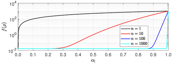
Figure 1.
Modification of turbulent viscosity based on the Reboud method for different values of the parameter n.
Instead of directly limiting the eddy viscosity, interfacial turbulence damping can be applied by introducing a source in the specific dissipation equation that mimics the influence of a wall. We apply the model developed by Frederix et al. [30], which is based on an improvement in Egorov’s approach [31]. With Egorov’s method, a source term is added to the equation
where is the interfacial-area density for phase i, is the cell height normal to the interface, and B is a user-defined damping factor with a default value of 10 [32]. Using the formulation Frederix et al. [30], the source term added in the interface regions for is written as
Also, here, the term A is an indicator field that is active only at the interface, and the dissipation source is given by
where is a length scale associated with turbulence damping at the interface. In the OpenFOAM implementation, instead of an indicator defined by Frederix et al. [30], an improved formulation was used for the term A:
where is a normal vector on the free surface evaluated at the face of a cell. It is computed from volume fraction gradients, and the dot product is then taken with the cell face normal; that is,
where is the cell face area vector. denotes the value of the volume fraction at the cell face, and denotes that in the center of the cell. We will refer to Frederix’s damping method as SST-D in the following.
Within this work, we also implemented Frederix’s damping method in FLUENT as a UDF, including an improved formulation for the coefficient A as in OpenFOAM. The source term is evaluated as the equations are solved, which does not cause significant computational overhead.
The hybrid RANS-LES turbulence modelling approaches employed in this study are also based on the SST model. The SAS approach strictly belongs to the unsteady RANS approaches and adjusts the turbulent length scale based on the local flow. The SAS model yields RANS solutions for stationary flows. In contrast, the model reduces eddy viscosity in zones with transient instabilities according to a von Kármán length scale that represents the locally resolved vortex size [44]. In the SAS model, a source term is added to the equation. The source term is
The von Kármán length scale is given by
The length scale is described as a ratio of the first and second derivatives of the velocity, where the first is represented by the strain rate invariant S, and the latter by the magnitude of the velocity Laplacian . The other model parameters and constants are given by Egorov and Menter [44].
2.2. Turbulence Modelling with LES-Based Methods
The subgrid-scale stress is modeled according to the Boussinesq hypothesis as , and using the wall-adapted local eddy viscosity model (WALE) by Nicoud and Ducros [45], the eddy viscosity is given as
where is the strain rate tensor for the resolved velocity field and is a traceless symmetric part of the square of the velocity gradient tensor, with .
2.3. Discretization and Numerical Methods
The flow equations are discretized using a collocated finite-volume method. Equations are solved sequentially using a PIMPLE algorithm that merges SIMPLE [46] and PISO [47] methods [48,49]. Three outer iteration loops are employed, with two to three PISO loops for the pressure equation in each outer iteration to ensure proper convergence. The tolerances for the residuals of the iterative solvers are set to for all variables, except for the void-fraction equations, for which the solver tolerances have been lowered to . All variables are discretized using second-order spatial schemes, with non-orthogonal correction applied for gradient terms. Specifically, the convection terms for the volume fractions are treated using a central difference scheme with a total variation diminishing (TVD) limiter to avoid excessive numerical diffusion and to ensure proper resolution and physical boundedness within the iterative solution. The convection terms of the momentum equation are treated using a hybrid scheme based on the local Courant number, , where a TVD-limited central difference scheme is used for , and a second-order upwind-biased scheme is used otherwise. Time-accurate simulations are performed to resolve the flow field. A first-order implicit scheme is applied to time derivatives. We note that first-order methods introduce more numerical diffusion than higher-order methods; however, applications of higher-order time integration methods have been shown to be very unstable, leading to solver divergence. In our approach, the time step was determined adaptively by a maximum Courant number of one in the vicinity of the foil, and in practice, this results in time steps of the order of μs.
2.4. Uncertainty Analysis
Grid sensitivity studies are performed for selected CFD simulations. Richardson extrapolation for error estimation can be applied to cases exhibiting monotonic convergence, and the GCI (grid convergence index) of Celik et al. [50] is utilized here. The method uses three different grids with refinement ratios between medium–fine and coarse–medium and the corresponding differences in integral quantities and , where is the solution on the kth grid. As a representative cell size on each grid, the inverse cubic root of the number of cells is used. The apparent order p of the method is calculated as
The term q is given by
where . The extrapolated value is calculated from
The error estimates are then obtained as follows: The approximate relative error is
the extrapolated relative error
and the fine-grid convergence index
3. Test Case
The test case applied is a hydrofoil in a cavitation tunnel, which is shown in Figure 2. The foil is attached to a board (Figure 3) on the side of the tunnel and is set at an angle of attack of (nose down). The main characteristics of the hydrofoil and tunnel configurations are listed in Table 1.
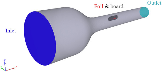
Figure 2.
Cavitation tunnel geometry with the foil and board, and inlet and outlet patches.
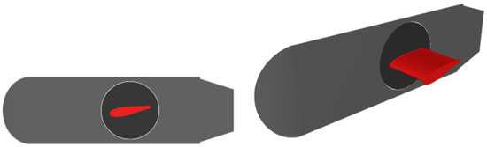
Figure 3.
Views of the hydrofoil in the tunnel.

Table 1.
Foil characteristics and tunnel configurations.
The cavitation tunnel features a converging geometry, characterized by a large inlet section and a tapering shape for the test section, where the hydrofoil is positioned. The desired flow speed and pressure, and thus the desired cavitation and Reynolds numbers, are set in the test section of the cavitation tunnel based on the Venturi effect, which is characterized by the accelerating fluid flow and decreasing pressure that occur in the converging tunnel. In the experiments, pressure probes are placed on the circumference of the tunnel near the inlet section and in the measurement section just before the foil and board, as shown in Figure 4, to measure the pressure levels. Based on the pressure levels, the flow speed can be determined using Bernoulli’s equation.
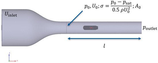
Figure 4.
Location of measurement section and specification of boundary and initial conditions.
Typically, in a CFD analysis, the designated velocity is assigned by the inflow boundary condition, and the outflow boundary condition sets the desired pressure level. In this case, the cavitation tunnel forms a Venturi tube, where the test section is located in the region of increased velocity. The speed in the test section, , is determined based on mass conservation, that is,
The cross-sectional areas are known, so the inflow speed can be determined by the desired speed in the test section . To determine the pressure in the test section, we carried out initial calibration CFD simulations, from which the axial pressure distribution from the test section to the outlet was approximated using a linear function. That is, based on the simulation, we obtained the pressure coefficient and its derivative . The pressure in the test section is adjusted in each case using this relation, or , where l is the distance between the outlet boundary patch and the test section, and is the pressure defined as the outlet BC in the CFD solver. Figure 5 shows typical convergences of pressure, flow speed, and cavitation number to the target values in the test section of the cavitation tunnel. As shown in Figure 5, the pressure was adjusted in the simulation to obtain the correct cavitation number at the test section, corresponding to the experiments. In the CFD method, the outlet pressure is specified, but in the experiments, the cavitation conditions were based on the probe data. Therefore, the outlet pressure was adjusted as described to reach the correct condition, which was monitored and validated in each simulation. The target speed in the test section is 19 m/s, giving a Reynolds number based on the foil chord of . The cavitation number is defined as
where is the saturation vapor pressure.
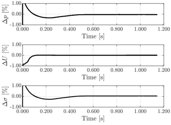
Figure 5.
Illustration of convergences of pressure, flow speed, and cavitation number to the target values at the test section.
Turbulence intensity I of 2% was used to approximate the turbulent kinetic energy at the inlet (). The inlet value for the specific dissipation was approximated from with approximated as ≈0.003 m. A no-slip condition is used on solid surfaces. Wall functions are applied to the turbulence fields, with a zero-gradient condition for k at the wall, and near-wall cell values for are set based on blending between the viscous sublayer (linear) and logarithmic turbulent boundary layer velocity profiles, which are functions of local wall distance values. Due to a large amount of simulations carried out using different CFD solvers, we have chosen to focus computational resources on the cavitation region instead of the wall region, where high resolution in each coordinate direction would be needed in a wall-resolved simulation. Spalding’s curve fit is used, from which can be evaluated. A zero-gradient condition is applied to the volume fractions at the walls, and a fixed flux condition is used for the pressure.
The mean global forces and visualization of cavity appearance are available from experiments under different flow conditions. Figure 6 shows an experimental observation of the cavitation appearance of the foil at . The sheet cavitation formed near the leading edge covers roughly a third of the chord, with its tail part then periodically transforming into cloudy, bubbly structures. Cavity shedding was observed, occurring roughly from slightly above the root to past the mid-span of the foil, as seen in the figure. The cloud cavities were convected to the wake and past the trailing edge of the foil. The steady region shown in the figure indicates the absence of cavity shedding behavior based on experimental observation, but its extent and closure shape fluctuated slightly. In addition, tip vortex cavitation occurs on both sides of the end plate.
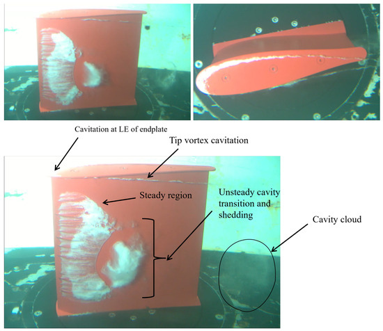
Figure 6.
Observations of cavitation extent and types at from experiments. The flow is from left to right.
Four grids were constructed for the case. The details of the grids are given in Table 2. Figure 7 shows the three CFD grids: coarse, medium, and fine. The grid cells were heavily clustered toward the hydrofoil and the end plate at the tip. The extra-fine grid was further refined for the end-plate region, as shown in Figure 8; otherwise, it is the same as the fine grid.
Table 2.
Details of grids used.
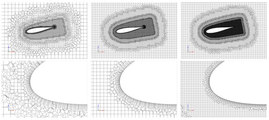
Figure 7.
Views of CFD grids near the foil and close to the LE. From left to right: coarse, medium, and fine grids.
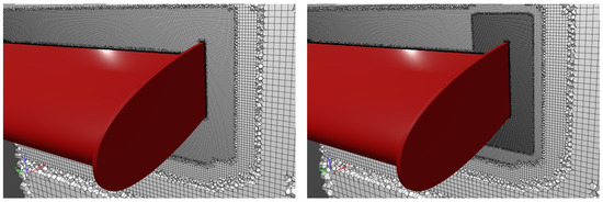
Figure 8.
Views of the fine and extra-fine CFD grids near the foil and the tip. On the left: fine grid. On the right: extra-fine grid.
4. Results
First, we present an overview of cavitation observations for the hydrofoil, following a sensitivity study of the SST-D and SST-R methods regarding the model parameters. Then, we present the results of uncertainty analyses concerning grid resolution using different turbulence modelling methods. The performance of the hydrofoil and the characteristics of transient cavitation are then investigated. Performance is mainly assessed using the lift coefficients , drag coefficients , and moment coefficients , defined as
where is the vertical force coefficient, is the horizontal force component, and is the moment about the y axis (span-wise axis), and the reference area is . The SST, SST-D, and SST-R methods are typically applied in conjunction with LES.
Summary of analysed conditions is given in Table 3. Most of the results presented in this study were obtained using the OpenFOAM computational fluid dynamics (CFD) solver. Selected operating conditions were also analyzed using FLUENT, where the same Schnerr–Sauer mass transfer model was employed with parameters identical to those used in the OpenFOAM simulations. To limit this study merely to the effect of the turbulence damping both in OpenFOAM and Fluent, we have tried to reproduce the previously used OpenFOAM numerical setup as closely as possible in Fluent. However, since Fluent is a closed-source commercial code, it is not likely to have an identical setup. A notable difference between the two codes is in the discretization of the volume fraction transport equation. OpenFOAM utilizes a multidimensional limiter scheme (MULES), while FLUENT employs a high-resolution interface capturing (HRIC) scheme. The idea in both discretizations is to retain a sharp interface between the phases while still allowing for reasonable numerical stability. It can be assumed that the Fluent implementation favors numerical stability more. In the FLUENT simulations, the standard SST turbulence model was used, as well as Egorov’s original damping approach—essentially Equation (14)—which we refer to as SST-E. Furthermore, simulations were performed using the improved damping method, SST-D, corresponding to Equation (15). Figure 9 presents snapshots that illustrate the extent and nature of cavitation based on experimental observations and OpenFOAM LES results, and Figure 10 shows the instantaneous velocity magnitude distribution near the hydrofoil.
Table 3.
Summary of analyzed conditions.
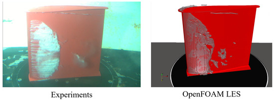
Figure 9.
Instantaneous snapshots from experiments and simulations depicting cavitation extent and types at .
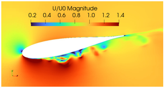
Figure 10.
Instantaneous snapshot of non-dimensional velocity magnitude from LES at .
In addition, we use a Strouhal number, defined as , where f is the sheet cavitation shedding frequency when discussing unsteady cavitation. We determined the frequency f from time histories and frequency domain analyses of hydrofoil forces and vapor volumes, as well as animations generated from the CFD simulations.
4.1. Effect of Parameters of Turbulence Damping Methods
We conducted a sensitivity analysis of the parameters and n in the SST-D and SST-R methods, respectively. Reboud’s method (SST-R) is an ad hoc approach to limit eddy viscosity levels for cavitating conditions. In contrast, the interfacial turbulence damping method (SST-D) is based on physical arguments that the phase interface behaves wall-like in segregated flows. Figure 11 shows the error in the CFD-predicted lift coefficient at using the coarse grid with respect to the different parameters. For reference, the applied SST method without damping gave an error of ; the SST method predicted the collapse of the lift force due to cavitation, which was not observed in the experiments.
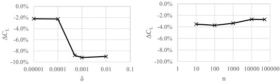
Figure 11.
Errors in CFD predicted lift coefficients with the SST-D (left) and SST-R (right) using different model parameters on a coarse grid. For reference, the SST method (without damping) gave an error of .
With the SST-D method, we varied the parameter to m. Figure 11 shows that significant improvements in simulation results can be achieved with appropriate values for , while excessively large values for the parameter do not enhance the results compared to the SST method. Applying greater values for reduces the influence of the additional source term in Equation (15) and reverts the behavior of the SST-D model towards the SST model. This resulted in steady cavitation on the foil. Damping of turbulence generation in the mixture region was insufficient for adequate shedding to occur. As seen in the figure, this yields similar errors in the lift coefficient as the SST model without any damping. Lowering the value improved the results, and the difference with respect to the experiments was about with on the coarse grid. Values below destabilized the simulations, likely because excessive damping of the turbulent eddy viscosity reduced the effective dissipation in the solution. Based on these results, we apply the value in all subsequent SST-D simulations. The maximum mean cavity thickness was about 5 mm, indicating that, for the present case, an appropriate interfacial turbulence damping length scale is on the order of the mean cavity thickness divided by 50. However, a deeper understanding of this interpretation in the context of cavitating flows requires further investigation. We note that the default value was , as given by Frederix et al. [30], which also produced good results in our case for mean lift and unsteady cavity shedding behavior.
For the SST-R method, we varied the parameter n as n ∈ [10, 50,000]. As we can see in Figure 11, the SST-R method gives relatively good results for all the parameters applied. Increasing the value toward improved the results, but increasing it further to n = 100,000 caused the simulations to become unstable and crash after a short time. The value was chosen for all subsequent SST-R simulations.
We also carried out, although not shown here, a brief sensitivity check with the FLUENT solver using the Egorov damping or SST-E method, focusing on the parameter B in Equation (14) and the foil lift force. We used values of , and 100. The results indicated that the force trends were not greatly affected by this parameter. This is likely since the coefficient influences the amount of damping applied, not where the damping is applied, which is dictated more by the indicator fields or A.
4.2. An Uncertainty Analysis
Grid sensitivity studies were carried out for SST, SST-D, SST-R, and LES. Here, the focus is on comparing the mean lift of the hydrofoil at as the integral quantity. A Richardson extrapolation for error estimation can be performed for cases exhibiting monotonic convergence, and we apply the GCI as described in Section 2.4.
Table 4 shows a comparison of the lift, drag, and moment coefficients with the experimental values under this condition. The moment about the y axis (span-wise axis) is evaluated at the mid-chord. The results of the grid sensitivity study are shown in Table 5 for different approaches to turbulence modelling. The cell counts of the grid were roughly M, M, and M, and the ratios were and .
Table 4.
Comparison of the force coefficients predicted with different turbulence modelling approaches on the fine grid at and the experimental value.
Table 5.
Calculation of numerical uncertainty and discretization error of the lift coefficient for different turbulence modelling approaches at . The experimental result was .
The SST method yields a significant error in all investigated integral quantities, particularly in the drag coefficient. Both SST-D and SST-R significantly improve the results compared to the SST method. The LES solution provides a very good match in the lift, drag, and moment coefficients compared to the experimental results. For LES, the approximate error is below 1 % and the fine-grid convergence index is 1%. The LES result, even on the coarse grid, is very close to the experimental value.
Moreover, the SST-D results are very similar across the different grids used, and the numerical uncertainty in the simulations is low, as determined by the GCI method. The approximate and extrapolated relative errors are below ca. 1% for the SST-D and LES methods. The SST-R method did not yield a monotonic convergence of the lift coefficient with grid refinement; consequently, most GCI characteristics cannot be determined from these results.
LES Solution Quality
An index of quality can be determined for LES solutions [51] as
where is the kinematic viscosity of the mixture and is the subgrid-scale eddy viscosity based on the LES solution. According to Celik et al. [51], values for the quality index greater than 0.8 indicate a good LES. Figure 12 shows that, based on , the quality of the solution is sufficient.
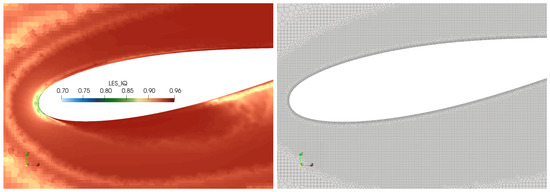
Figure 12.
On the left: for fine-grid cavitating LES at . On the right: only the grid cells are shown for reference.
4.3. Hydrofoil Performance and Cavitation Observation
The results in terms of the lift coefficients are given in Figure 13 as functions of the cavitation number. The figure displays the experimental data alongside the simulation results obtained using various turbulence modelling methods and CFD solvers. The results in are summarized in Table 6 on different grids, turbulence models, and flow solvers for mean lift, drag, and moment coefficients. In the table, the frequencies and the corresponding Strouhal numbers are also given. If there is no apparent variation in the forces or cavitation volume, the result is denoted as steady. Figure 14 also shows the mean vapor volume as a function of the cavitation number using the different turbulence modelling methods from the OpenFOAM simulations.
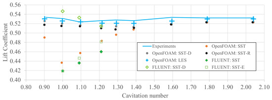
Figure 13.
Lift coefficients at different cavitation numbers and turbulence modelling methods on the medium grid.
Table 6.
Comparison of simulation results on the coarse, medium, fine, and extra-fine grids using different turbulence modelling methods with the experiments at . Most results are obtained using the OpenFOAM solver, and coarse-grid solutions of FLUENT simulations with various methods are also included.
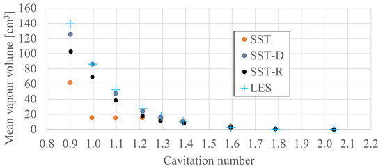
Figure 14.
Mean vapor volume as a function of the cavitation number. Medium-grid OpenFOAM simulations with different turbulence modelling methods.
The LES method yields consistent results for hydrofoil performance across different grid resolutions and exhibits low sensitivity to grid refinement. Overall, LES results remain slightly below the experimental measurements, with a deviation of less than 1%. As noted above, accurately resolving the near-wall region in high-Reynolds-number flows requires excellent mesh resolution in all directions, particularly in wall-resolved simulations. To properly evaluate this aspect, not only is a detailed experimental uncertainty analysis necessary but also a substantial increase in the number of computational cells near the wall is required. The LES consistently provides the closest match to the experimental results across all applied grid resolutions. Even on the coarse grid, the LES results are very close to the experimental values. The SST-D method offers improved accuracy compared to the SST and SST-R methods, particularly in capturing cavity dynamics. The force and moment values are close to the experimental results with all applied grids using the SST-D. It is also less sensitive to variations in grid resolution, as the results are consistent across different grid resolutions, with errors that are comparable to those in the experiments. SST-R shows an improvement over the SST method; however, it does not yield results as accurately as SST-D or LES. The SST and SST-R methods exhibit moderate sensitivity to grid resolution, and predictions improve with finer grids. SST-R lacks monotonic convergence with grid refinement, making uncertainty quantification difficult, although the predicted lift values are close to the experimental results on all applied grids. Especially on the coarse and medium grids, the SST-R gives poor results for drag. The SST method is the least accurate, as it under-predicts lift and over-predicts drag, especially on coarse and medium grids. It also produces essentially steady results and does not capture unsteady cavitation shedding. When applying the SST-SAS method, which belongs to hybrid RANS-LES modelling strategies, cavity dynamics are not predicted without the damping method, even with the fine grid. In fact, when the damping is applied (SST-SAS-D), the results are very close to the LES solution in terms of the global forces.
The FLUENT results denoted as SST-E in Figure 13 and in Table 6 correspond to the Egorov damping method. This existing Egorov’s turbulence damping method in the FLUENT solver slightly improves the results, but the lift still drops under the investigated conditions, and no cavitation shedding is observed. FLUENT results with the SST-D method significantly improve the results, now also producing the shedding of the cavity. Although the OpenFOAM and FLUENT results are not identical, the damping implemented in FLUENT no longer causes the lift force to crash under high cavitation conditions. The SST-D with FLUENT predicts an overestimation of lift at lower cavitation numbers.
All models show a sharp increase in the vapor volume as the cavitation number drops below ≈ 1.6–1.8 in Figure 14, marking the onset of cavitation. Before this point, the vapor volume is negligible, and all models behave similarly. LES and SST-D show similar trends in the amount of cavitation in Figure 14. Both models predict higher vapor volumes at lower cavitation numbers, and the curves are closely aligned. Compared to SST-D and LES, the SST-R model shows lower vapor volumes, especially at lower ’s. The standard SST model predicts the lowest vapor volumes. It also shows less sensitivity to changes in . Before cavitation inception, which occurs between ≈ 1.6 and 1.8 as seen in Figure 14, the lift predicted by the different SST methods overlaps. This is, of course, expected when cavitation is absent and no modifications are active for the source (SST-D) or the eddy viscosity (SST-R), which is roughly 1% below the experimental values. The non-cavitating lift values predicted by the LES method are very close to the experimental results, with differences of 0.5 % or less. The best overall agreement with the experimental data is obtained throughout the investigated range of conditions using the LES method. The results obtained with different variants of the SST method (SST, SST-D, and SST-R) are relatively close to each other in wetted conditions and begin to diverge as the cavitation number decreases. When damping is included, the sheet cavity breaks, creating a longer-reaching low-pressure region on the suction side, which helps retain the lift of the hydrofoil and provides a better match with the measurements. Among the RANS-based methods, the SST-D model yields the best overall agreement with the experimental results. The SST-R results with OpenFOAM are slightly lower than the corresponding SST-D results. Without damping, the kinetic energy of the turbulence, as predicted by the models, has higher values, which eventually lead to a more extensive and uniform cavitation region. Without any damping, the lift decreases nearly linearly with the cavitation number, a phenomenon observed with both the OpenFOAM and FLUENT solvers. There is a small systematic under-prediction of lift using LES and SST-D methods throughout the investigated range of cavitation numbers.
SST-D is similar to the LES result in terms of mean gas volume, compared to the SST-R model in Figure 14. When cavitation formation is not substantial enough, the use of additional damping with the SST method does not notably influence mean foil performance. This is evident for cases with approximately . Even the fine-grid LES was insufficient to predict the tip vortex cavitation accurately; the grid resolution near the tip was too coarse to capture the low-pressure peak in the fine vortex core. In the finest grid simulations, the cavitation of the tip vortex is visible (Figure 9). It is also interesting to note that, using the LES method, the results of global forces and their dynamics based on time history analyses were very similar for all grids. Even the coarse-grid LES produced a tiny deviation from the experimental result and the solution of the finest grid LES. Although the grid spacing affects the resolution of turbulent spectra, the current meshes appear to be appropriate for the WALE approach. Future work on this topic will be necessary.
Figure 15 shows the observation of cavitation from experiments and CFD simulations. Different turbulence modelling methods were applied to the fine grid. The SST method predicts steady cavitation with very mild oscillation at the cavity closure near the mid-span of the foil. Other methods predict that unsteady cavity shedding will occur from the root of the foil to slightly past the mid-span, with notable vapor structures shedding into the wake of the foil. The LES and SST-D methods predict cavity structures that convect quite far past the leading edge of the foil, whereas the SST-R method exhibits greater dissipation, with the vapor region condensing back into water closer to the mid-chord. Moreover, the LES and SST-D show a similar convex shape of cavity closure when the main cloud is broken off, which is in good agreement with visual observations made from the experiments. With the SST-R method, the dynamic shape of the cavity closure is not very clear.
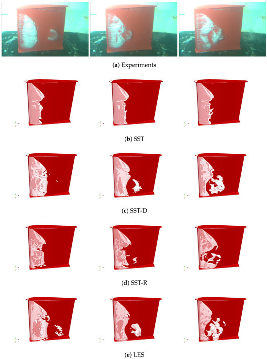
Figure 15.
Cavitation observation from experiments and fine-grid CFD solutions at using different turbulence modelling methods.
4.4. Transient Cavitation Features
Figure 16 shows the results in the time and frequency domains, as well as the RMS fluctuation of vapor volume presented as bars using the different turbulence modelling methods. Figure 17 compares the mean and instantaneous cavitation appearances of the SST and SST-D methods, showing a slight variation with SST and notably larger unsteady behavior with SST-D. The SST result in the time domain is nearly a flat black curve in Figure 16, indicating that there is not much change in the vapor volume as a function of time. There is no frequency domain content and no unsteady cavitation shedding, whereas results from the other methods (SST-D, SST-R, and LES) show an apparent variation with time. In fact, the SST-D result is somewhat similar to the LES solution in the sense that the mean amount of vapor is also elevated compared to the SST solution, and the time and frequency domain results have a similar shape. However, the amplitude of fluctuation is lower with the SST-D method than with the LES method. Higher-order harmonics in gas volume fluctuation are visible in both the SST-D and LES solutions of similar amplitude. The magnitudes of the amplitudes and dominant frequencies differ slightly, with Hz and 57 Hz for SST-D and LES, respectively. These correspond to Strouhal numbers of ≈ 0.56–0.59. LES results and SST-D results on finer grids have shown periodic shedding with . This was also predicted using the SST-D method on the finer grids. Although detailed experimental results on time-resolved cavitation dynamics are not available, experimental observations and video recordings indicate clear cavity cloud shedding under this condition ().
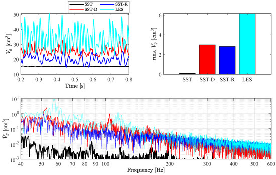
Figure 16.
Time and frequency domain CFD results of vapor volume with different turbulence modelling methods on a coarse grid at .
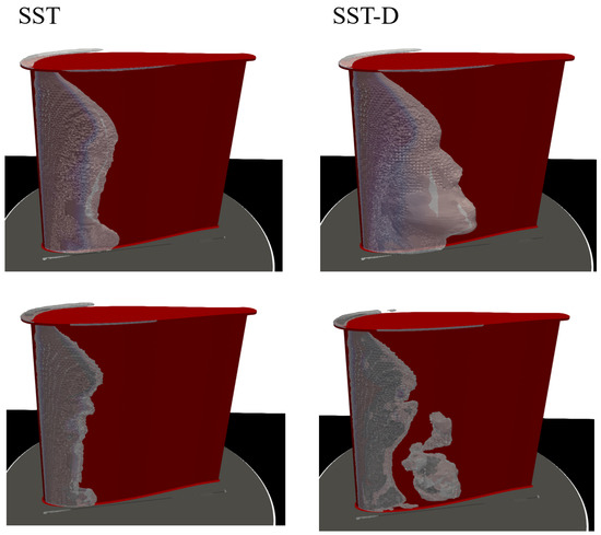
Figure 17.
Mean (top row) and instantaneous (bottom row) cavitation appearance from SST and SST-D methods using the coarse grid at .
Based on experimental observations and video recordings, we assessed the stability of the cavity, focusing on the shedding of the sheet cavity into the slipstream of the hydrofoil. Snapshots of some conditions are shown in Figure 18. The experiments showed that the attached sheet cavitation on the hydrofoil was stable for approximately . Notable cavitation shedding began to occur when this value was approximately four or less, with an increasing amount of vapor being shed as this value decreased, as seen in Figure 18. These observations are consistent with those discussed by Leroux et al. [52], who experimentally studied a NACA hydrofoil under cavitating conditions and showed that a limit for which the stable cavity transitions to an unstable cavity is , which they accredit as Arndt et al. [53] criteria (cf. Figure 19). In fact, a potential flow solution for steady cavitating hydrofoils [54] gives unsteady partial cavities for approximately . In addition to the experimental results presented here, the simulations with all the turbulence modelling approaches considered show a similar behavior, which is visible, for example, as a clearly increased RMS fluctuation in Figure 19 of the total volume of the vapor for approximately or . In addition, throughout the investigated range of cavitation numbers, the RMS fluctuation of the gas volume is at a level similar to that of the SST-D and LES solutions. The SST method clearly does not produce fluctuations even as the cavitation number decreases and only shows an increased RMS level at the lowest investigated cavitation condition, . This could also explain the anomaly of the higher mean lift force obtained with the SST in Figure 13 at the lowest .
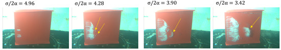
Figure 18.
Observation of cavitation extent at different values of . Snapshots from experimental video recordings, with arrows indicating a detaching cavity cloud from the main sheet.
Figure 19.
Classification of stable and unsteady cavitation (left) with markers showing simulated conditions, and RMS. fluctuation of gas volume (right) with different turbulence modelling methods. The secondary x axis on the right graph shows corresponding values of the parameter .
Figure 20 shows the mean volume fraction near the foil on a cut plane at mid-span over a time span of 0.5 s, covering roughly 30 cavity shedding cycles for the different turbulence modelling methods. The figure also illustrates the corresponding rms. fluctuations of the volume fraction fields over this time period, comparing the variability in the volume fraction using the different turbulence models. We note, however, that cavitation on the foil was highly three-dimensional and varied significantly with chordwise and spanwise locations. However, comparisons at the cross-section provide helpful insights into the performance and behavior of the different models. Table 7 shows the cavity lengths determined from these results. Note that these lengths, especially the values from the tests, contain some uncertainty, as they are visually determined and measured based on video recordings or from the averaged CFD simulation results. In the figure, the mean cavitation extents are very similar between the SST-D and LES methods. In addition, their shapes and local vapor contents are similar between these methods. The SST model yields a considerably shorter mean extent, accompanied by a significantly larger vapor concentration near the foil surface, extending up to the cavity closure. Compared to experiments, SST under-predicts cavity length and shows minimal fluctuation. The SST-R predicts a thinner mean cavity shape with a lower vapor concentration compared to the SST-D and LES methods. The cavity fluctuation is also very similar between the SST-D and LES methods. Their shapes and vapor concentrations are nearly identical, with LES showing a slightly more elongated extent of the cavity oscillations in dilute regions with very low vapor content. The SST-R produces significantly less variability in the cavity, with different vapor concentration profiles as well. With the SST method, some oscillation occurred only near the closure of the sheet cavity, without any shedding of vapor structures to the wake. Based on the cavity-length results, the SST-D and LES are, again, closest to the experimental result. In addition, the methods give similar magnitudes for the fluctuating extent, as is also visible in Figure 20.
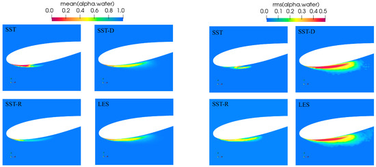
Figure 20.
Mean (left) and rms. fluctuation (right) volume fraction values at a cut plane on the mid-span from fine-grid CFD solutions using different turbulence modelling methods at .
Table 7.
Cavity lengths from different turbulence modelling methods at on the fine grid. The CFD results correspond to Figure 20.
Figure 21 shows the pressure coefficient () and non-dimensional turbulent kinetic energy () predicted using different models. The figure displays two instantaneous snapshots at different stages of cavity shedding, obtained from simulations for each turbulence model. The SST-D method significantly reduces the modeled turbulent kinetic energy compared to the SST and SST-R methods. The SST method generates a large amount of turbulent kinetic energy, with an increasing trend toward the cavity closure and downstream from it. The SST method yields large k levels well before cavity closure, whereas the SST-R exhibits a similar increase, albeit more pronounced at cavity closure. The SST-D method, then again, shows minimal production of k within the two-phase region. Cavitation shedding and oscillation are also visible in fluctuations in the pressure coefficient values on the foil surface. All models predict low levels of k within the cavity, that is, in areas with a higher vapor content.
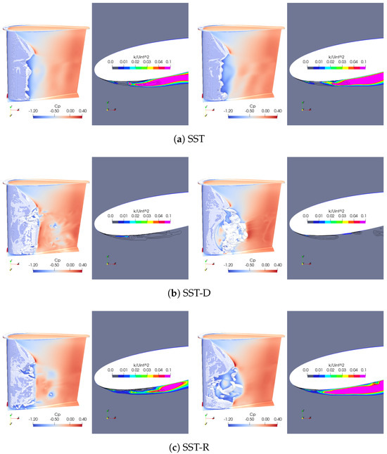
Figure 21.
The pressure coefficient on the foil, volume fraction isosurface, and non-dimensional turbulent kinetic energy on a cut plane at mid-span from fine-grid CFD solutions at using different turbulence modelling methods. Two different instantaneous snapshots from the simulations are shown for each turbulence model at two stages of cavity shedding. The zoomed views near the leading edge also show contours of as the black curves.
Figure 22 shows the mean ratios near the foil on a cut plane at mid-span over a time span of 0.5 s, covering roughly 30 cavity shedding cycles for the different turbulence modelling methods. Lower values of near the cavity interface indicate better resolution of the unsteady cavitation dynamics; excessive eddy viscosity can suppress important flow instabilities. Turbulence damping methods (SST-D and SST-R) and LES provide lower eddy viscosity levels compared to those of the standard SST-RANS model. The SST-R method reduces levels compared to SST, and the SST-D method produces considerably lower magnitudes. In particular, the predicted eddy viscosity level in the wake of the cavity is similar between the SST and SST-R methods but significantly lower for the SST-D method.
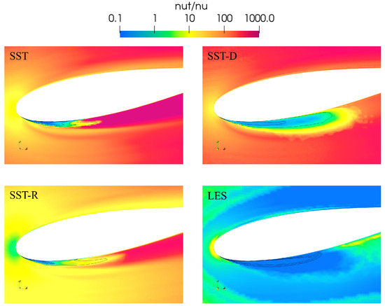
Figure 22.
Mean of ratios at a cut plane on the mid-span from fine-grid CFD solutions using different turbulence modelling methods at . Contours of are shown as the black curves.
5. Conclusions and Future Work
We have studied hydrofoil cavitation using several turbulence modelling methods and different flow solvers. We applied VOF mixture modelling for multiphase flow. In the experiments and simulations carried out here, the cavitation conditions ranged from wetted to fully cavitating; the Reynolds number was .
It is a known issue that two-equation turbulence models, without modification for cavitating flow configurations, are typically unable to accurately predict unsteady cavitation due to the over-prediction of eddy viscosity levels. An ad hoc Reboud limiter (here referred to as SST-R) for the eddy viscosity is commonly used in the case of these turbulence models. In addition to this method, we applied Egorov’s interfacial turbulence damping, as improved by Frederix et al. [30], which formulates interfacial damping based on physical arguments regarding the wall-like behavior of phase interfaces. This method is referred to as SST-D here.
Both the OpenFOAM and FLUENT solvers, using the SST turbulence model, fail to predict key cavitation phenomena, such as lift breakdown and unsteady cavity shedding. The application of turbulence damping for RANS-based methods significantly improved the simulation results.
The SST-D method significantly improved predictions by reducing eddy viscosity near the cavity interface, a key feature in capturing unsteady cavitation dynamics, including cloud shedding. The SST-D method showed good agreement with the experimental data. The SST-R method also improved the results over the SST; however, in our study, it was less effective than the SST-D, showing greater dissipation and less variability in the vapor structures. Limiting turbulence production with RANS methods in the two-phase region allows for more transient effects to occur. This enabled cavitation shedding to occur, allowing the vapor to break off from the suction side of the hydrofoil and preventing the breakdown of the lift force as the cavitation number was lowered. Additionally, cavitating flow simulations using the FLUENT solver with the SST-D method yield significantly improved results. The LES method WALE provided the most accurate and consistent results in all grid resolutions in the present study.
The SST-D and SST-R have additional user-defined parameters that control the damping of turbulence fields. We conducted a parameter study to determine their effects and sensitivities. The values applied for most of our analyses were for the SST-D method and n = 10,000 for the SST-R method. Based on our results, SST-D appeared more sensitive to the choice of the dimensional interface length scale than the SST-R method was to the selection of the exponent parameter n. The identification of an interface’s presence is determined algorithmically using the SST-D method. Using SST-R, only an algebraic relation based on phase densities or volume fractions is used, making it numerically less complex as well. Although it has not yet been widely used for cavitating flow problems, the SST-D approach for accounting for multiphase turbulent flow has a more physically based justification than eddy viscosity damping methods.
The LES method provided very accurate results on all grids applied here for global forces. The SST-D method yielded practically similar results on all applied grids for the global forces, whereas the SST-R method produced an oscillatory result as the grid was refined. Both the SST-D and LES methods produced good results on all grids concerning the mean forces and moments of the foil, as well as the dynamic behavior of the cavity. This suggests that the coarsest grid applied was sufficient for these methods to achieve good global performance predictions. However, we note that the SST model and the LES exhibited more evident monotonic convergence of the mean forces towards the experimental values. It is unanticipated that almost no difference in terms of mean forces was observed with the SST-D method between the grids. This warrants a more detailed investigation of the grid convergence properties of SST-D when applied to cavitating problems. An extra-fine grid was constructed to resolve the fine cavitating tip vortex. Future research is needed to expand the scope of test cases for parameter and grid sensitivity studies, as well as to include different cases of varying complexity, such as ship propulsors.
Author Contributions
Writing—original draft, V.V.; Writing—review & editing, P.P., M.N., J.H. and T.S. All authors have read and agreed to the published version of the manuscript.
Funding
This research received no external funding.
Data Availability Statement
The original contributions presented in this study are included in the article. Further inquiries can be directed to the corresponding author.
Acknowledgments
The authors would like to express their gratitude for the support granted by Business Finland in the project “UltraPropulsor”. The authors wish to acknowledge VTT’s HPC cluster (“The Doctor”) and CSC—IT Center for Science, Finland, for computational resources.
Conflicts of Interest
Author V. Viitanen is employed by the company VTT Technical Research Centre of Finland Ltd.; Author Mika Nuutinen is employed by ABB Marine and Ports. The remaining authors declare that the research was conducted in the absence of any commercial or financial relationships that could be construed as a potential conflict of interest.
References
- Brennen, C. Fundamentals of Multiphase Flow; Cambridge University Press: Cambridge, UK, 2005. [Google Scholar]
- Ge, M.; Svennberg, U.; Bensow, R. Investigation on RANS prediction of propeller induced pressure pulses and sheet-tip cavitation interactions in behind hull condition. Ocean Eng. 2020, 209, 107503. [Google Scholar] [CrossRef]
- Lidtke, A.; Lloyd, T.; Lafeber, F.; Bosschers, J. Predicting cavitating propeller noise in off-design conditions using scale-resolving CFD simulations. Ocean Eng. 2022, 254, 111176. [Google Scholar] [CrossRef]
- Asnaghi, A.; Svennberg, U.; Bensow, R. Large eddy simulations of cavitating tip vortex flows. Ocean Eng. 2020, 195, 106703. [Google Scholar] [CrossRef]
- Viitanen, V.M.; Hynninen, A.; Sipilä, T.; Siikonen, T. DDES of Wetted and Cavitating Marine Propeller for CHA Underwater Noise Assessment. J. Mar. Sci. Eng. 2018, 6, 56. [Google Scholar] [CrossRef]
- Cheng, H.; Long, X.; Ji, B.; Peng, X.; Farhat, M. LES investigation of the influence of cavitation on flow patterns in a confined tip-leakage flow. Ocean Eng. 2019, 186, 106115. [Google Scholar] [CrossRef]
- Asnaghi, A.; Bensow, R.; Svennberg, U. Comparative analysis of tip vortex flow using RANS and LES. In Proceedings of the MARINE VII: Proceedings of the VII International Conference on Computational Methods in Marine Engineering, Nantes, France, 15–17 May 2017; pp. 836–847. [Google Scholar]
- Sipilä, T.; Sánchez-Caja, A.; Siikonen, T. Eddy vorticity in cavitating tip vortices modelled by different turbulence models using the RANS approach. In Proceedings of the 6th European Conference on Computational Fluid Dynamics, (ECFD VI), Barcelona, Spain, 20–25 July 2014. [Google Scholar]
- Viitanen, V.M.; Siikonen, T. Numerical simulation of cavitating marine propeller flows. In Proceedings of the 9th National Conference on Computational Mechanics (MekIT’17), Trondheim, Norway, 11–12 May 2017; International Center for Numerical Methods in Engineering (CIMNE): Barcelona, Spain, 2017; pp. 385–409, ISBN 978-84-947311-1-2. [Google Scholar]
- Balaras, E.; Schroeder, S.; Posa, A. Large-eddy simulations of submarine propellers. J. Ship Res. 2015, 59, 227–237. [Google Scholar] [CrossRef]
- Lu, N.X.; Bensow, R.E.; Bark, G. Large eddy simulation of cavitation development on highly skewed propellers. J. Mar. Sci. Technol. 2014, 19, 197–214. [Google Scholar] [CrossRef]
- Usta, O.; Korkut, E. A study for cavitating flow analysis using DES model. Ocean Eng. 2018, 160, 397–411. [Google Scholar] [CrossRef]
- Hynninen, A.; Viitanen, V.; Tanttari, J.; Klose, R.; Testa, C.; Martio, J. Multiphase Flow Simulation of ITTC Standard Cavitator for Underwater Radiated Noise Prediction. J. Mar. Sci. Eng. 2023, 11, 820. [Google Scholar] [CrossRef]
- Reboud, J.L.; Stutz, B.; Coutier, O. Two phase flow structure of cavitation: Experiment and modelling of unsteady effects. In Proceedings of the 3rd International Symposium on Cavitation CAV1998, Grenoble, France, 7–10 April 1998; Volume 26, pp. 1–8. [Google Scholar]
- Gnanaskandan, A.; Mahesh, K. Large eddy simulation of the transition from sheet to cloud cavitation over a wedge. Int. J. Multiph. Flow 2016, 83, 86–102. [Google Scholar] [CrossRef]
- Coutier-Delgosha, O.; Fortes-Patella, R.; Reboud, J.L. Evaluation of the turbulence model influence on the numerical simulations of unsteady cavitation. J. Fluids Eng. 2003, 125, 38–45. [Google Scholar] [CrossRef]
- Zhang, X.L.; Ge, M.M.; Zhang, G.J.; Coutier-Delgosha, O. Compressible effects modelling for turbulent cavitating flow in a small venturi channel: An empirical turbulent eddy viscosity correction. Phys. Fluids 2021, 33, 035148. [Google Scholar] [CrossRef]
- Decaix, J.; Goncalves, E. Time-dependent simulation of cavitating flow with k − ε turbulence models. Int. J. Numer. Methods Fluids 2012, 68, 1053–1072. [Google Scholar] [CrossRef]
- Coutier-Delgosha, O.; Stutz, B.; Vabre, A.; Legoupil, S. Analysis of cavitating flow structure by experimental and numerical investigations. J. Fluid Mech. 2007, 578, 171–222. [Google Scholar] [CrossRef]
- Vaz, G.; Lloyd, T.; Gnanasundaram, A. Improved modelling of sheet cavitation dynamics on Delft Twist11 hydrofoil. In Proceedings of the MARINE VII: Proceedings of the VII International Conference on Computational Methods in Marine Engineering, Nantes, France, 15–17 May 2017; pp. 143–156. [Google Scholar]
- Leclercq, C.; Archer, A.; Fortes-Patella, R.; Cerru, F. Numerical cavitation intensity on a hydrofoil for 3D homogeneous unsteady viscous flows. Int. J. Fluid Mach. Syst. 2017, 10, 254–263. [Google Scholar] [CrossRef]
- Peters, A.; Sagar, H.; Lantermann, U.; el Moctar, O. Numerical modelling and prediction of cavitation erosion. Wear 2015, 338, 189–201. [Google Scholar] [CrossRef]
- Melissaris, T.; Bulten, N.; Van Terwisga, T. A numerical study on the shedding frequency of sheet cavitation. In Proceedings of the MARINE VII: Proceedings of the VII International Conference on Computational Methods in Marine Engineering, Nantes, France, 15–17 May 2017; pp. 801–812. [Google Scholar]
- Melissaris, T.; Schenke, S.; Van Terwisga, T.J. Cavitation erosion risk assessment for a marine propeller behind a Ro–Ro container vessel. Phys. Fluids 2023, 35, 013342. [Google Scholar] [CrossRef]
- Li, D.; Grekula, M.; Lindell, P. A modified SST k − ω turbulence model to predict the steady and unsteady sheet cavitation on 2D and 3D hydrofoils. In Proceedings of the 7th International Symposium on Cavitation, Ann Arbor, MI, USA, 16–20 August 2009. [Google Scholar]
- Li, D.; Grekula, M.; Lindell, P. Towards numerical prediction of unsteady sheet cavitation on hydrofoils. J. Hydrodyn. 2010, 22, 699–704. [Google Scholar] [CrossRef]
- Ji, B.; Luo, X.; Arndt, R.; Wu, Y. Numerical simulation of three dimensional cavitation shedding dynamics with special emphasis on cavitation–vortex interaction. Ocean Eng. 2014, 87, 64–77. [Google Scholar] [CrossRef]
- Zhou, L.; Wang, Z. Numerical simulation of cavitation around a hydrofoil and evaluation of a RNG κ-ε model. J. Fluids Eng. 2008, 130, 011302. [Google Scholar] [CrossRef]
- Huuva, T.; Törnros, S. Computational fluid dynamics simulation of cavitating open propeller and azimuth thruster with nozzle in open water. Ocean Eng. 2016, 120, 160–164. [Google Scholar] [CrossRef]
- Frederix, E.; Mathur, A.; Dovizio, D.; Geurts, B.; Komen, E. Reynolds-averaged modelling of turbulence damping near a large-scale interface in two-phase flow. Nucl. Eng. Des. 2018, 333, 122–130. [Google Scholar] [CrossRef]
- Egorov, Y.; Boucker, M.; Martin, A.; Pigny, S.; Scheuerer, M.; Willemsen, S. Validation of CFD Codes with PTS-Relevant Test Cases; 5th Euratom Framework Programme ECORA Project; European Commission: Brussels, Belgium, 2004; Volume 2004, pp. 91–116. [Google Scholar]
- ANSYS FLUENT User’s Guide; Ansys Inc.: Canonsburg, PA, USA, 2023.
- Kunz, R.; Boger, D.; Chyczewski, T.; Stinebring, D.; Gibeling, H.; Govindan, T. Multi-phase CFD analysis of natural and ventilated cavitation about submerged bodies. In Proceedings of the 3rd ASME-JSME Joint Fluids Engineering Conference, San Francisco, CA, USA, 18–23 July 1999; p. 13. [Google Scholar]
- Schnerr, G.; Sauer, J. Physical and numerical modelling of unsteady cavitation dynamics. In Proceedings of the Fourth International Conference on Multiphase Flow (ICMF), New Orleans, LA, USA, 27 May–1 June 2001; Volume 1. [Google Scholar]
- Merkle, C.; Feng, J.; Buelow, P. Computational modelling of the dynamics of sheet cavitation. In Proceedings of the 3rd International Symposium on Cavitation, Grenoble, France, 7–10 April 1998; Volume 2, pp. 47–54. [Google Scholar]
- Zwart, P.; Gerber, A.; Belamri, T. A two-phase flow model for predicting cavitation dynamics. In Proceedings of the Fifth International Conference on Multiphase Flow, Yokohama, Japan, 30 May–4 June 2004; Volume 152. [Google Scholar]
- Saito, Y.; Takami, R.; Nakamori, I.; Ikohagi, T. Numerical analysis of unsteady behavior of cloud cavitation around a NACA0015 foil. Comput. Mech. 2007, 40, 85. [Google Scholar] [CrossRef]
- Niedźwiedzka, A.; Schnerr, G.; Sobieski, W. Review of numerical models of cavitating flows with the use of the homogeneous approach. Arch. Thermodyn. 2016, 37, 71–88. [Google Scholar] [CrossRef]
- Luo, X. and Ji, B. and Tsujimoto, Y. A review of cavitation in hydraulic machinery. J. Hydrodyn. 2016, 28, 335–358. [Google Scholar] [CrossRef]
- Menter, F.; Esch, T. Elements of industrial heat transfer predictions. In Proceedings of the 16th Brazilian Congress of Mechanical Engineering, Uberlandia, Spain, 26–30 November 2001. [Google Scholar]
- Menter, F.R.; Kuntz, M.; Langtry, R. Ten Years of Industrial Experience with the SST Turbulence Model. In Turbulence, Heat and Mass Transfer 4; Hanjalic, K., Nagano, Y., Tummers, M., Eds.; Begell House, Inc.: Danbury, CT, USA, 2003; pp. 625–632. [Google Scholar]
- Launder, B.E.; Spalding, B. The numerical computation of turbulent flows. Comput. Methods Appl. Mech. Eng. 1974, 3, 269–289. [Google Scholar] [CrossRef]
- Coutier-Delgosha, O.; Reboud, J.; Delannoy, Y. Numerical simulation of the unsteady behaviour of cavitating flows. Int. J. Numer. Methods Fluids 2003, 42, 527–548. [Google Scholar] [CrossRef]
- Egorov, Y.; Menter, F. Development and application of SST–SAS model in the DESIDER project. In Advances in Hybrid RANS-LES Modelling; Notes on Numerical Fluid Mechanics and Multidisciplinary Design; Springer: Berlin/Heidelberg, Germany, 2008; Volume 97. [Google Scholar]
- Nicoud, F.; Ducros, F. Subgrid-scale stress modelling based on the square of the velocity gradient tensor. Flow Turbul. Combust. 1999, 62, 183–200. [Google Scholar] [CrossRef]
- Caretto, L.; Gosman, A.; Patankar, S.; Spalding, D. Two calculation procedures for steady, three-dimensional flows with recirculation. In Proceedings of the Third International Conference on Numerical Methods in Fluid Mechanics: Vol. II Problems of Fluid Mechanics, Paris, France, 3–7 July 1972; Springer: Berlin/Heidelberg, Germany, 1973; pp. 60–68. [Google Scholar]
- Issa, R. Solution of the implicitly discretised fluid flow equations by operator-splitting. J. Comput. Phys. 1986, 62, 40–65. [Google Scholar] [CrossRef]
- Weller, H. Pressure-Velocity Solution Algorithms for Transient Flows; OpenCFD Ltd.: Reading, UK, 2005. [Google Scholar]
- Greenshields, C.; Weller, H. Notes on Computational Fluid Dynamics: General Principles; CFD Direct Ltd.: Reading, UK, 2022. [Google Scholar]
- Celik, I.; Ghia, U.; Roache, P.; Freitas, C. Procedure for estimation and reporting of uncertainty due to discretization in CFD applications. J. Fluids Eng.-Trans. ASME 2008, 130, 078001. [Google Scholar]
- Celik, I.B.; Cehreli, Z.N.; Yavuz, I. Index of Resolution Quality for Large Eddy Simulations. J. Fluids Eng. 2005, 127, 949–958. [Google Scholar] [CrossRef]
- Leroux, J.B.; Astolfi, J.; Billard, J. An experimental study of unsteady partial cavitation. J. Fluids Eng. 2004, 126, 94–101. [Google Scholar] [CrossRef]
- Arndt, R.; Song, C.; Kjeldsen, M.; He, J.; Keller, A. Instability of partial cavitation: A numerical/experimental approach. In Proceedings of the 23rd Symposium on Naval Hydrodynamics, Val de Reuil, France, 17–22 September 2000. [Google Scholar]
- Acosta, A. A Note on Partial Cavitation of Flat Plate Hydrofoils; Hydrodynamics Laboratory Report E-19.9; California Institute of Technology: Pasadena, CA, USA, 1955. [Google Scholar]
Disclaimer/Publisher’s Note: The statements, opinions and data contained in all publications are solely those of the individual author(s) and contributor(s) and not of MDPI and/or the editor(s). MDPI and/or the editor(s) disclaim responsibility for any injury to people or property resulting from any ideas, methods, instructions or products referred to in the content. |
© 2025 by the authors. Licensee MDPI, Basel, Switzerland. This article is an open access article distributed under the terms and conditions of the Creative Commons Attribution (CC BY) license (https://creativecommons.org/licenses/by/4.0/).