Neural Network-Based Prediction of Wave Pressure Distribution on Hyperbolic Paraboloid Surfaces

Abstract

Recent studies have demonstrated the potential of hyperbolic paraboloid (hypar), a doubly curved geometry, in coastal engineering applications. Predicting pressure distribution, critical for subsequent finite element analysis, on such novel three-dimensional structures require Computational Fluid Dynamics (CFD) simulations, which are computationally intensive. To address this challenge, the current study develops an artificial neural network (ANN) surrogate to predict pressure distributions on hypar free-surface breakwaters (FSBWs) under solitary wave loading. Using Smoothed Particle Hydrodynamics (SPH) as the CFD tool, simulations generate the supervised learning dataset, where inputs are the hypar warping $R_n$, breakwater draft $d_r$, and wave height $H$. The targets consist of two $30\times 30$ pressure maps at wave arrival (hydrostatic) and peak, together with the wave rise time $\left\{\mathit{P}\right(t_0)$, $\mathit{P}\left(t_{peak}\right)$, $\mathsf{\Delta }t=t_{peak}-t_0\}$. Three architectures, FNN, CNN, and DeepONet, are trained with homoscedastic uncertainty loss weighting, each at two parameter sizes ($~50\mathrm{k}$ and $~500\mathrm{k}$). Results for training and testing show that all models achieve low errors, with models with ~50k parameters found to be sufficient, and scaling to ~500k yields some generalization improvement. Further reducing the parameters (~5k) degrades accuracy for all models, with DeepONet proven most robust to parameter size reduction. Overall, this study introduces a novel SPH-ANN workflow for predicting wave pressures on hypar FSBWs, where inference on new samples occurs in a few milliseconds per sample, delivering orders-of-magnitude speedups relative to running new SPH simulations. This computational efficiency enables rapid design iteration and optimization of hypar FSBWs, facilitating their potential deployment in coastal defense.

1. Introduction

The Intergovernmental Panel on Climate Change (IPCC) findings indicate a significant rise in mean sea levels due to global warming [1]. In addition, studies on climate model projections show that tropical cyclones are likely to become more intense as the planet warms [2,3]. These trends, rising seas, and stronger storms, underscore an urgent need to improve the resilience of coastal infrastructure and hence call for innovative coastal defense systems.

Traditional coastal defenses, such as massive bottom-standing breakwaters, have limitations in this context; while they are effective at wave attenuation, bottom-standing breakwaters demand large volumes of construction material and disrupt local marine ecosystems and sediment transport processes [4]. In deeper waters, their construction and maintenance become especially costly and challenging [5,6,7]. These drawbacks call for alternative breakwater designs that are more sustainable and adaptable. Free-surface breakwaters (FSBWs) have emerged as one potential type of alternative to conventional designs [7]. FSBWs are situated at the water surface (where wave energy is concentrated) and attenuate incoming waves mainly through reflection and dissipation. Therefore, FSBWs can be moored or pile-mounted without blocking water flow below them, avoiding the environmental and material drawbacks of conventional breakwaters [7,8].

The geometric profile of coastal structures plays a key role in determining performance and has been widely studied for their effects on force reduction, wave attenuation, and other processes [9,10,11,12,13,14]. In recent years, there has been growing research interest in FSBW designs exploring various shapes such as H-, U-, or T- cylindrical and pontoon forms, or other novel front faces to improve wave attenuation [8,15,16,17,18,19]. Most prior studies on FSBW geometry have focused on enhancing wave energy dissipation, with fewer examining the structural response of these new forms [20,21,22]. In the context of enhancing wave attenuation and structural performance in FSBWs, one form that has been innovatively adopted is the hyperbolic paraboloid (hypar) [20].

Hypar surfaces are doubly curved shell geometries (Figure 1) known for their structural efficiency, with one direction acting as “arches” that carry compressive forces from the shell’s corners toward its vertex, balanced by a “cable” carrying tensile forces in the perpendicular direction [23,24,25]. This arch-and-cable mechanism enables the hypar shell to achieve smaller thickness than a flat plate of the same span. Despite its doubly curved shape, a hypar surface has straight-line generators in two directions, meaning the formwork and reinforcement can be constructed from straight elements [23,26]. This property was greatly utilized in the mid-20th century by the renowned designer Félix Candela in thin concrete shell roofs [25].

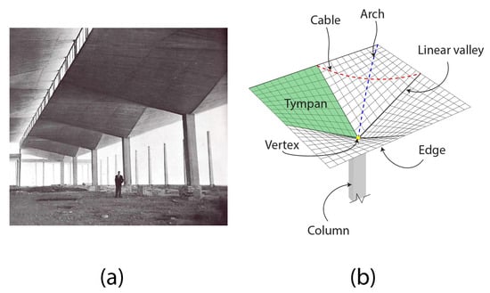
Figure 1. Four-edged hypar umbrella used as a roof. (a) Real-world example from the Rio’s Warehouse, designed by Félix Candela in Mexico around 1954; image courtesy of Princeton University Library’s Department of Special Collections. (b) Hypar shell illustrating arch-and-cable, tympan, and straight-line generators.

More recently, researchers are revisiting hypar forms not only for roofs but also for coastal structures, recognizing their advantages in new applications. For instance, Wang et al. [27] proposed a deployable hypar canopy which serves as a public shade under normal conditions and rotates into a vertical coastal barrier during storm surges. Using decoupled SPH (Smoothed Particle Hydrodynamics)-FEM (Finite Element Modeling) simulations, the authors showed that the hypar’s negative Gaussian curvature reduces bending moments, shear forces, and peak stresses by promoting membrane action over bending [27]. In a related work, Wu et al. [28] used a decoupled SPH-FEM scheme to analyze a segment of a hypar coastal barrier. The study found that wave pressures follow a bilinear-like height distribution with peaks concentrated near the longitudinal spine, and that simplified methods (e.g., Goda’s formula) under-predict peak pressures and structural responses for the hypar barrier surface [28]. Additionally, Smith et al. [20] extended hypar applications to FSBWs by conducting hydrodynamic and structural evaluation of fixed hypar-faced FSBWs (Figure 2) using a similar SPH-FEM framework validated against 1:10 experimental flume tests. For the operating wave periods ($T\le 6 \mathrm{s}$) and drafts, transmission coefficient was reduced by up to 50% and peak shell stresses by an order of magnitude versus flat-faced counterparts, confirming hypar’s dual advantage for coastal defense [28].

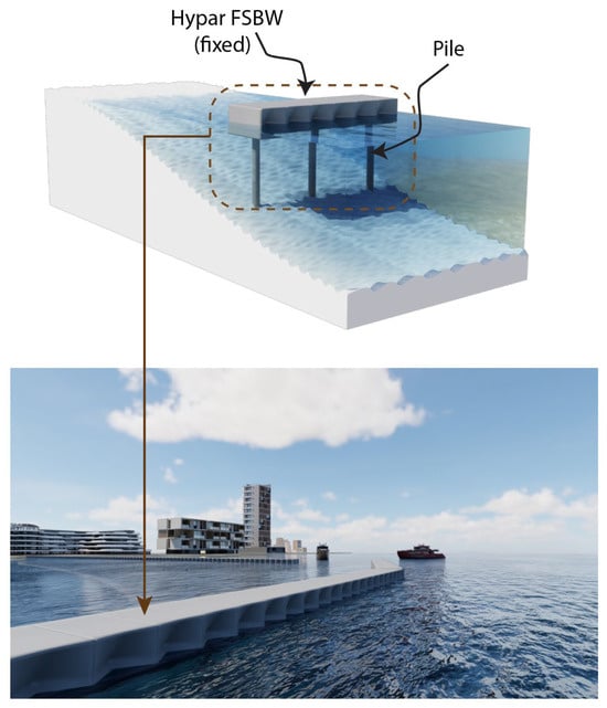
Figure 2. Rendering of a fixed, pile-supported hypar FSBW array, leeside protected region (e.g., harbor/marina) to the left and seaward to the right.

These studies [20,27,28] used SPH for the hydrodynamic analysis and pressure probing because it excels at free-surface flows and complex fluid–structure interactions (FSIs). SPH can capture breaking waves, water impact, and irregular geometries, such as hypar shells, without the meshing issues of grid-based CFD [29,30,31]. However, SPH is computationally intensive. For example, Smith et al. [20] reported that when using High-Performance Computing (HPC), equipped with Nvidia A100, ~600 clock seconds elapse to simulate 1 s of SPH time. This limitation motivates developing machine learning (ML) models that, once trained, can accurately and rapidly predict pressure distributions on hypar and similarly complex 3D (three-dimensional) coastal geometries.

Recent studies increasingly apply ML in coastal engineering, developing surrogate models that accelerate analysis and design by replacing computationally intensive simulations with fast predictions from surrogate models; see [32] for an in-depth review. In breakwaters applications, artificial neural networks (ANNs) have been used to predict wave reflection [33], transmission [34], and overtopping [35], often performing better than empirical formulas. In a study related to the deployable hypar umbrella barrier [27], Smith et al. [23] used genetic programming (GP) to accurately predict the deflection of N-edged hypar shells under normal (i.e., acting as shade) conditions, by training the GP model on a large dataset of FEM simulations. However, no prior work has developed models for wave-induced pressure distributions on hypar shells or other novel doubly curved coastal structures, which are the inputs for subsequent FEM analysis [20]. The goal of this study is to addresses that gap by developing a framework for neural network-based surrogates, trained on SPH simulation data, to predict wave pressure distributions on hypar FSBWs.

The remainder of this study is organized as follows: Section 2 presents the workflow and methodology. Section 3 presents the workflow implementation and models’ performance results. Section 4 summarizes the key findings and conclusions.

2. Methodology

Building on previous work demonstrating the effectiveness of hypar surfaces for FSBWs [20], this study develops an SPH-ANN framework to predict pressure distributions on hypar FSBWs subjected to solitary waves. The hypar FSBWs are modeled as fixed, consistent with common practice in coastal engineering, particularly hypar structures [20,27,28,36]. The workflow, summarized in Figure 3a, begins with parametric hypar FSBW generation in Rhino/Grasshopper (Figure 3b), parameterized by normalized rise $R_n$ and draft $d_r$. DualSPHysics [29] is then used to run SPH simulations in which solitary waves of prescribed height $H$ interact with the hypar FSBW.

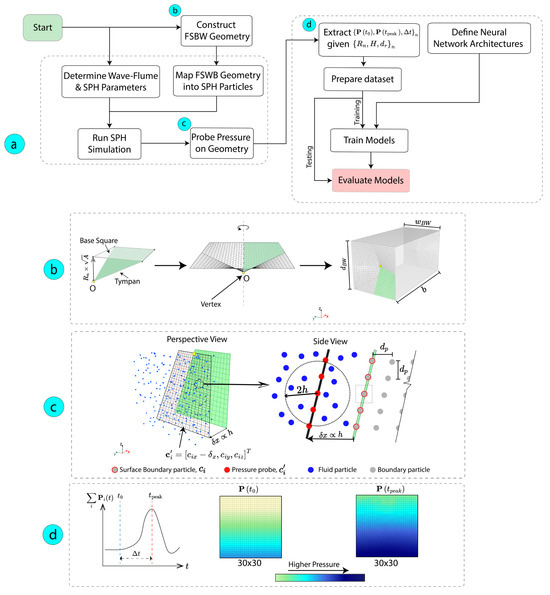
Figure 3. SPH-Neural methodology for predicting wave pressure distribution on hypar FSBWs. (a) Workflow showing hypar FSBW geometry generation and SPH analysis to neural networks evaluation. (b) Parametric hypar geometry (Rhino/Grasshopper) with warping described by normalized rise, $R_n$. (c) Seaside pressure probing in SPH. (d) Post-processing for extracting target outputs.

For each sample, pressures on the seaside surface are probed (Figure 3c) and post-processed to extract relevant pressure distribution data for the subsequent supervised learning task. Three ANN architectures are trained and evaluated: feedforward neural network (FNN) [37], convolutional neural network (CNN) [38], and Deep Operator Network (DeepONet) [39]. This section details each step of this methodology.

2.1. Smoothed Particle Hydrodynamics Formulation

SPH is a Lagrangian, mesh-free technique that represents a continuum with discrete particles and computes the governing equations at a specific point from neighboring particles’ contributions [29,30]. SPH is well suited to free-surface flows, large deformations, and complex geometries [30,31], which explains its use in FSI analyses of hypar structures [20,27,28]. The SPH approximation of a scalar field $F$ (e.g., pressure or a velocity component) at particle $a$ is given by the following:

$$F\left({\mathbf{r}}_a\right)\approx \sum _b F\left({\mathbf{r}}_b\right){\displaystyle \frac{m_b}{{\rho }_b}}W\left({\mathbf{r}}_a-{\mathbf{r}}_b,h\right),$$

(1)

where $m_b$ and ${\rho }_b$ are the mass and density of neighbor $b$, $\mathbf{r}$ denotes the particle position at which $F$ is evaluated, $W$ is the smoothing kernel with compact support, and $h$ is the smoothing length. Similarly to previous work on hypar FSBWs [20], the Quintic Wendland kernel [40], which has a support vanishing beyond $2h$, is adopted this study. Refer to DualSPHysics documentation [29] for more details.

2.2. Navier–Stokes Equations and Boundary Treatment

The study uses a weakly compressible SPH (WCSPH) that considers the Navier–Stokes equations in the discrete form as implemented in DualSPHysics [29]:

$${\displaystyle \frac{d{\mathbf{v}}_a}{dt}}=-\sum _b m_b\left({\displaystyle \frac{p_a}{{\rho }_a^2}}+{\displaystyle \frac{p_b}{{\rho }_b^2}}\right){\nabla }_a{W}_{ab}+\mathbf{g}+{\mathsf{\Gamma }}_a,$$

(2)

$${\displaystyle \frac{d{\rho }_a}{dt}}=\sum _b m_b{\mathbf{v}}_{ab}\cdot {\nabla }_a{W}_{ab}+D,$$

(3)

with $\mathbf{v}$ representing velocity, $p$ representing pressure, $\rho$ representing density, $\mathbf{g}$ representing gravity, ${\mathsf{\Gamma }}_{\mathrm{a}}$ representing artificial viscosity at $a$ [30], and $D$ as a density-diffusion term to regularize density fluctuations [41]. In WCSPH, pressure is calculated from density using Tait type equation of state [42]:

$$p={\displaystyle \frac{c_s^2{\rho }_0}{\gamma }}\left[{\left({\displaystyle \frac{\rho }{{\rho }_0}}\right)}^{\gamma }-1\right],$$

(4)

where $c_s=\sqrt{\partial p/\partial \rho }$ is the numerical speed of sound, $\gamma =7$ the polytropic exponent, and ${\rho }_0$ the reference density [29].

In DualSPHysics, time stepping follows the symplectic position Verlet scheme with a predictor–corrector stage and adaptive time stepping to satisfy the Courant–Friedrich–Lewy (CFL) condition [29,43].

In this study, fluid–boundary interactions are handled with the Dynamic Boundary Condition (DBC) in DualSPHysics, consistent with prior work on hypar coastal structures [20,27,44]. In DBC, solid boundaries (e.g., flume walls, breakwater faces) are discretized into boundary particles (Figure 3c) that use the same SPH equations as the fluid but are kinematically constrained, that is, are in a fixed or prescribed motion [29,30,45]. When a fluid particle enters a boundary particle’s kernel support, the boundary particle’s density—and hence pressure via the equation of state (Equation (4))—increases, generating a repulsive pressure term in the momentum equation (Equation (2)).

2.3. Solitary Wave Generation

Solitary waves are generated using the Boussinesq-based wavemaker theory developed by Goring [46] and implemented in DualSPHysics [29], which models the wave piston as a moving boundary. The formulation equates the depth-averaged particle velocity under the wave crest to the piston velocity [46]. This yields a law of motion for the piston displacement in time, $x_s\left(t\right)$, which can be solved iteratively [29]. The depth-averaged velocity at the wavemaker is defined as follows:

$$u\left(x_s,t\right)={\displaystyle \frac{c\eta \left(x_s,t\right)}{h+\eta \left(x_s,t\right)}}={\displaystyle \frac{d{x}_s}{dt}},$$

(5)

Integrating both sides of the above equation gives the piston displacement as follows [46]:

$$x_s(t)={\displaystyle \frac{2H}{kh}}\mathrm{t}\mathrm{a}\mathrm{n}\mathrm{h}\left[k\left(ct-x_s\left(t\right)\right)\right],$$

(6)

with the associated solitary wave free-surface profile,

$$\eta \left(x_s,t\right)=H{\mathrm{s}\mathrm{e}\mathrm{c}\mathrm{h}}^2\left[k\left(ct-x_s\right)\right].$$

(7)

In these equations, $H$ is the target solitary wave height, $h$ is the still-water depth, $c$ is the wave celerity, $k$ is the outskirt coefficient, and $\eta$ is the free-surface elevation. Note that in this implementation, only $H$ is specified to generate the solitary wave, with the wave period $T$ computed implicitly, so $T$ need not be included as an additional parameter. For further details, see Goring [46] and the DualSPHysics documentation [29].

2.4. Hypar FSBW Geometry Generation

A parametric workflow in Grasshopper, a visual programming environment in Rhino [47], is used to generate the hypar FSBW geometry and to export models for SPH analysis and pressure probe locations [20]. Similarly to Smith et al. [20], the study considers a four-edged hypar geometry defined by the parameters normalized as rise $R_n$ and plan area $A = { d_{BW}\times w}_{BW}$ (breakwater depth and width, respectively); see Figure 3b. A single tympan is constructed from a base square of plan $A/4$. Vertex O is displaced by the hypar rise $R_e = Rn\times \surd A$ along the negative z-direction; for example, $R_n=0$ yields a flat surface. The tympan is then arrayed four times around the center to form the complete four-edged hypar of total plan $A$. The resulting surface is assigned to the seaside and leeside faces of a box-type FSBW with dimensions ${b\times w}_{BW}\times d_{BW}$ (length, width, depth), as indicated in Figure 3b. Hypar FSBWs with specified $R_n$ and draft $d_r$ are then exported to DualSPHysics, where they are discretized into particles for hydrodynamic analysis and subjected to a solitary wave of height $H$.

2.5. Supervised Learning for Pressure Prediction

2.5.1. Pressure Probing and Dataset Construction

For the supervised learning task, pressure values are extracted via post-processing in DualSPHysics. As shown in Figure 3c, pressure probes ${\mathit{c}}_i’$ with a total count of $30\times 30=900$ are placed at an offset $\delta x$ in front (seaside) of the boundary particles ${\mathit{c}}_{\mathit{i}}$, consistent with previous work [20]. Next, the sum of the pressures $\sum _i{\mathit{P}}_i\left(t\right),$ where i is the ith probe, for each time step $t$ is plotted over the SPH simulation time (Figure 3d). A Butterworth low-pass filter (LPF) is applied to $\sum _i{\mathit{P}}_i\left(t\right)$ to remove high-frequency numerical noise [48]. Two time steps of interests are determined as follows: $t_0$, which is the arrival time of the wave at the FSBW surface, and $t_{peak}$, at which the sum of pressures is maximized (Equation (8)). To determine $t_0$, an initial baseline window is first used to compute the mean of the filtered total pressure $\sum _i{\mathit{P}}_i\left(t\right)$, and the wave arrival time $t_0$ is defined as the first time step instant, after this baseline window, at which the filtered total pressure $\sum _i{\mathit{P}}_i\left(t\right)$ exceeds a small threshold above its baseline mean; this threshold-based definition is commonly used in coastal engineering and tsunami studies [49], with implementation details provided in Section 3.1. From these two time steps $t_0$ and $t_{peak}$, rise time of the wave $\mathsf{\Delta }t$ is also calculated (Equation (9)). The corresponding pressure maps, $\mathit{P}\left(t_0\right)$ and $\mathit{P}\left(t_{peak}\right)$ are then extracted, each forming a 30 × 30 grid. These three outputs $\left\{\mathit{P}\right(t_0)$, $\mathit{P}\left(t_{peak}\right)$, $\mathsf{\Delta }t$} together with their corresponding inputs {$R_n$, $d_r$, $H$} form the dataset pair for the supervised learning task.

$$t_{peak}=\underset{\mathrm{t}}{\mathrm{a}\mathrm{r}\mathrm{g}\mathrm{m}\mathrm{a}\mathrm{x}}\sum _i{\mathit{P}}_i\left(t\right)$$

(8)

$$\mathsf{\Delta }t=t_{peak }-t_0$$

(9)

2.5.2. Loss Function and Optimization

The networks in this study must learn two targets with different scales and units, pressure maps values $\left\{\mathit{P}\right(t_0)$, $\mathit{P}\left(t_{peak}\right)\}$ on the order of thousands of pascals, and wave rise time, $\mathsf{\Delta }t$, on the order of a few seconds. To account for these differences, the total loss $\mathcal{L}$ adopts a homoscedastic uncertainty weighting, based on Kendall et al. [50], as follows:

$$\mathcal{L}={\displaystyle \frac{1}{2{\sigma }_{\mathit{P}}^2}}{L}_{\mathit{P}}+{\displaystyle \frac{1}{2{\sigma }_{\mathsf{\Delta }t}^2}}{L}_{\mathsf{\Delta }t}+\mathrm{l}\mathrm{o}\mathrm{g}{\sigma }_{\mathit{P}}+\mathrm{l}\mathrm{o}\mathrm{g}{\sigma }_{\mathsf{\Delta }t}$$

(10)

with

$$L_{\mathit{P}}={\displaystyle \frac{1}{N}}\sum _{n=1}^N \sum _{i=1}^{900} \left[{\left({\mathit{P}}_{i,n}{\left(t_0\right)}^{\mathrm{p}\mathrm{r}\mathrm{e}\mathrm{d}}-{\mathit{P}}_{i,n}{\left(t_0\right)}^{\mathrm{g}\mathrm{t}}\right)}^2+{\left({\mathit{P}}_{i,n}{\left(t_{\mathrm{p}\mathrm{e}\mathrm{a}\mathrm{k}}\right)}^{\mathrm{p}\mathrm{r}\mathrm{e}\mathrm{d}}-{\mathit{P}}_{i,n}{\left(t_{\mathrm{p}\mathrm{e}\mathrm{a}\mathrm{k}}\right)}^{\mathrm{g}\mathrm{t}}\right)}^2\right],$$

(11)

and

$$L_{\mathsf{\Delta }t}={\displaystyle \frac{1}{N}}\sum _{n=1}^N {\left(\mathsf{\Delta }{t}_n^{\mathrm{p}\mathrm{r}\mathrm{e}\mathrm{d}}-\mathsf{\Delta }{t}_n^{\mathrm{g}\mathrm{t}}\right)}^2$$

(12)

where $L_{\mathit{P}}$ is the mean-squared error (MSE) between predicted “pred” and ground-truth (or SPH) “gt” pressures $\mathit{P}$, $L_{\mathsf{\Delta }t}$ is the MSE for the wave rise time $\mathsf{\Delta }t$, ${\sigma }_{\mathit{P}}^2$ and ${\sigma }_{\mathsf{\Delta }t}^2$ are learnable noise homoscedastic variances, ${\mathit{P}}_{i,n}\left(\mathrm{t}\right)$ denotes the pressure value at probe $i$ of sample $n$ at time $t$, and $N$ is training batch size.

In this approach, minimizing $\mathcal{L}$ is equivalent to maximizing the joint likelihood (Gaussian for MSE) under a homoscedastic uncertainty assumption, meaning each task has a constant observation-noise scale, which removes the need for manual loss weight tuning [50].

All network parameters are optimized with Adam [51], an adaptive-momentum stochastic gradient method. Kaiming initialization [52] is used for all models in this study.

2.5.3. Neural Network Architectures

For the supervised learning task, the inputs are the normalized rise, breakwater draft, and wave height $\{R_n, d_r, H\}$, and the outputs are two 30 × 30 pressure maps and the wave rise time $\left\{\mathit{P}\right(t_0)$, $\mathit{P}\left(t_{peak}\right)$, $\mathsf{\Delta }t$}. This study employs three ANN architectures, shown in Figure 4: (a) FNN, (b) CNN, and (c) DeepONet. For each neural network architecture, two model sizes are considered, obtained by adjusting the latent dimensions within each architecture. See the Section 3 for implementation.

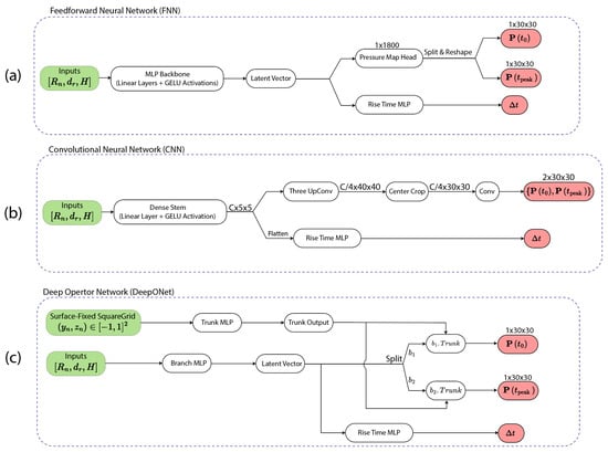
Figure 4. Neural Network Architectures to predict pressure maps $\left\{\mathit{P}\right(t_0)$, $\mathit{P}\left(t_{peak}\right)$} and wave rise from $\mathsf{\Delta }t$ from input parameters {$R_n$, $d_r$, $H$}: (a) FNN with MLP backbone and two heads, (b) CNN with a dense stem and a transposed-conv for pressure maps, with a parallel $\mathsf{\Delta }t$ head, and (c) DeepONet combining branch (input parameters) and trunk (grid) to produce pressure maps, with a parallel $\mathsf{\Delta }t$ head.

Although two model sizes are examined, the main purpose of this study is to demonstrate the SPH-ANN pressure prediction workflow rather than to identify a superior architecture or size. Designers are encouraged to choose the model architecture and size that best suits their specific tasks. Each architecture is briefly described as follows:

• FNN serves as a baseline which can approximate continuous mappings well [37]. From the inputs, as shown in Figure 4a, a shared multilayer perceptron (MLP) with GELU (Gaussian Error Linear Unit) [53] activations produces a latent vector, from which two heads branch: a linear head that outputs 1 × 1800 values reshaped into two 30 × 30 pressure maps {$\mathit{P}\left(t_0\right)$, $\mathit{P}\left(t_{peak}\right)\}$ and a small MLP head for $\mathsf{\Delta }t$.
• CNN is used as it has a spatial inductive bias which is useful for image-like fields [38]. As shown in Figure 4b, a dense stem embeds the inputs into a $5\times 5\times C$ latent representation. Transposed-convolution upsampling blocks expand the latent representation to $40\times 40$, followed by a center crop to $30\times 30$, and finally a $1\times 1$ convolution produces the two-channel pressure maps. In parallel, an MLP working on the latent representation produces $\mathsf{\Delta }t$.
• DeepONet is utilized for operator learning ability, mapping inputs to the outputs over a specified grid [39]. As shown Figure 4c, the branch MLP encodes $\{R_n, d_r, H\}$, and the trunk MLP encodes square-grid coordinates $(y_n,z_n)\in [-\mathrm{1,1}{]}^2$ attached to the FSBW surface, where probe location $(-1, -1)$ denotes the bottom-left and $(+1, +1)$ the top-right on the hypar surface. The dot product between branch and trunk embeddings yields the two pressure maps {$\mathit{P}\left(t_0\right)$, $\mathit{P}\left(t_{peak}\right)\}$. An additional MLP head working on the branch latent predicts $\mathsf{\Delta }t$.

The homoscedastic uncertainty weighting loss, Equation (10), is adopted to due to the difference in output scales [50]. In this study, however, $\mathsf{\Delta }t$ is produced by a dedicated MLP head in the architectures (Figure 4), so the homoscedastic uncertainty weighting loss may be proven unnecessary for accurate $\mathsf{\Delta }t$ prediction. Section 3.6 assesses whether such loss weighting in Equation (10) is required.

3. SPH-ANN Workflow Implementation

This section presents the detailed implementation of SPH data generation and ANN training workflow, shown in Figure 3, for pressure prediction on hypar FSBWs.

3.1. SPH Setup and Parameters

For this implementation, the hypar FSBW dimensions are held fixed and follow previous work by the authors [20], which experimentally validated the SPH simulations for hypar FSBW FSIs using a 1:10 prototype. The FSBW dimensions are hence set to length $b=10 \mathrm{m}$, depth $d_{BW}=5 \mathrm{m}$, and width $w_{db}=5 \mathrm{m}$ (see Figure 3b). As summarized in Table 1, the input parameters {$R_n$, $d_r$, $H$} are sampled on a full-factorial grid [54] within the operating range for FSBWs [4,20,21]: $R_n$ varies from 0.0 (flat surface) to 0.50 in 0.125 increments; $d_r$ from 0.0 m (bottom of the breakwater at the still-water level) to 5.0 m (fully submerged) in 1.25 m increments; and $H$ from 1.2 m to 2.4 m in 0.3 m increments. In total, 125 SPH simulations are carried out.

In this study, note that the trained neural networks (Section 3.2), with non-polynomial activation functions, can perform inference on arbitrary continuous values of $(R_n, d_r, H$) within the trained parameter range. This continuous function approximation ability is established by the Universal Approximation Theorem [55] and validated empirically by the test set results in Section 3.4.

Table 1. SPH parameters of study (bold indicates variable parameters, which serve as inputs for supervised learning).

	Parameter	Values
Geometric Properties (See Figure 3)	Normalized rise, ${\mathit{R}}_{\mathit{n}}$	0, 0.125, 0.25, 0.375, 0.50
	Breakwater length, b (m)	10
	Breakwater width, $w_{BW}$ (m)	5
	Breakwater depth, $d_{BW}$ (m)	5
Wave and Bathymetry (See Figure 5)	Wave Height, $\mathit{H}$ (m)	1.2, 1.5, 1.8, 2.1, 2.4
	Breakwater draft, ${\mathit{d}}_{\mathit{r}}$ (m)	0, 1.25, 2.5, 3.75, 5.0
	Water depth, $d$ (m)	10

Table 1. SPH parameters of study (bold indicates variable parameters, which serve as inputs for supervised learning).

	Parameter	Values
Geometric Properties (See Figure 3)	Normalized rise, ${\mathit{R}}_{\mathit{n}}$	0, 0.125, 0.25, 0.375, 0.50
	Breakwater length, b (m)	10
	Breakwater width, $w_{BW}$ (m)	5
	Breakwater depth, $d_{BW}$ (m)	5
Wave and Bathymetry (See Figure 5)	Wave Height, $\mathit{H}$ (m)	1.2, 1.5, 1.8, 2.1, 2.4
	Breakwater draft, ${\mathit{d}}_{\mathit{r}}$ (m)	0, 1.25, 2.5, 3.75, 5.0
	Water depth, $d$ (m)	10

Figure 5. Wave flume SPH setup: (a) elevation view and (b) top view. The pressure probes ${\mathit{p}}_i$ are placed only in front of the central FSBW section.

SPH parameters, such as the wave height to interparticle spacing ratio $H/d_p$ and the pressure probe offset $\delta x$ from the boundary particles, follow Smith et al. [20]. Hence, the interparticle spacing $d_p$ is set to 0.065 m to maintain $H/d_p\ge 18$ for all wave heights, and the pressure probe is offset to $\delta x=3 \mathrm{h}$. Each of the 125 simulations is run on high-performance hardware, at Princeton Research Computing, using an NVIDIA A100 GPU and a 2.6 GHz AMD EPYC Rome CPU. Simulating $30$ s of physical time requires approximately 80 h. Table 2 summarizes the SPH numerical setup and device settings.

Table 2. SPH parameters and device configuration.

Attribute.	Values
Kernal type	Quintic Wendland kernel
Boundary Method	Dynamic Boundary Condition (DBC)
Interparticle distance ($d_p$)	$\le H/18$
Probe offset ($\delta x)$	$3 \mathrm{h}$
Artificial viscosity coefficient	0.01 (near irrotational flows)
Clock time per SPH time (s/s)	~10,000
GPU	NVIDIA A100
CPU	2.6 GHz AMD EPYC Rome

Figure 6 illustrates one SPH run {$R_n=0.5, d_r=2.5 \mathrm{m}, H=1.8 \mathrm{m}$} as an example. As discussed in the methodology section, the total pressure $\sum _i{\mathit{P}}_i\left(t\right)$ is plotted, from which $t_0$ and $t_{peak}$ are identified and $\mathsf{\Delta }t$ is computed. In this study, the baseline window is taken over the first 5 s of each SPH run, and $t_0$ is defined as the first instant at which the filtered total pressure exceeds 5% above this baseline mean. Thresholds between 3% and 10% produced similar $t_0$ values, so 5% was adopted for all simulation outputs; the corresponding implementation is available in the repository cited in the Data Availability statement. The corresponding pressure maps $\mathit{P}\left(t_0\right)$ and $\mathit{P}\left(t_{peak}\right)$ are then extracted. Inputs and outputs from 125 (Table 1) of such runs form the dataset used for the supervised learning task described in the next subsection.

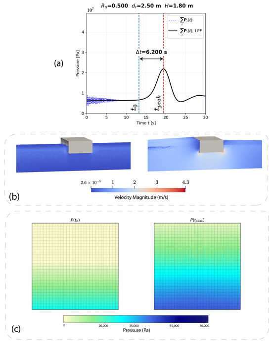
Figure 6. Example SPH case ($R_n=0.5, d_r=2.5 \mathrm{m}, H=1.8 \mathrm{m}$): (a) time history of sum of pressures $\sum _i{\mathit{P}}_i$; (b) visualization snapshots at $t_0$ and $t_{peak}$; and (c) extracted pressure maps $\mathit{P}\left(t_0\right)$ and $\mathit{P}\left(t_{peak}\right)$.

3.2. ANN Models’ Training Settings

Supervised learning is performed with the three ANN architectures introduced in Section 2.3: FNN, CNN, and DeepONet. The inputs are {$R_n$, $d_r$, $H$} and the outputs are two 30 × 30 pressure maps and a scalar rise time $\left\{\mathit{P}\right(t_0)$, $\mathit{P}\left(t_{peak}\right)$, $\mathsf{\Delta }t\}$. For each architecture, two model sizes are considered, with parameter counts of approximately 50k (±10%) and 500k (±10%).

Training settings are summarized in Table 3. As described in Section 2.5, the loss uses homoscedastic uncertainty weighting to balance the pressure maps and rise time targets without the need for manual tuning [50]. This implementation uses the Adam optimizer with the commonly used [51,56] learning rate of ${10}^{-3}$ and weight decay ${10}^{-4}$, with a cosine-annealing schedule [57]. Weight decay and early stopping are used to mitigate overfitting, which is assessed using the test dataset results in Section 3.4. All models are trained with a batch size of 6 for a max of 4000 epochs and early stopping in case of no improvement. Training each model takes less than 3 min, run locally on a PC equipped with an NVIDIA RTX 3080 Ti (CUDA) and an Intel Core i9-10900k CPU. Trained models perform inference in under $2 \mathrm{m}\mathrm{s}$. All scripts and data are available in the public repository referenced in the Data Availability statement.

Table 3. ANN training hyperparameters and settings.

Component	Setting
Optimizer	Adam
Learning rate	${10}^{-3}$
Weight decay	${10}^{-4}$
Learning rate schedule	Cosine decay
Activation	GELU
Initialization	Kaiming
Max epochs	4000
Batch size	6
Dataset split	100 training/25 test samples (80%/20%)
Base loss	MSE for both pressure and rise time
Loss weighting	Homoscedastic uncertainty weighting
Device	CUDA on NVIDIA RTX 3080 Ti
Training time per model	3 min
Inference time per sample	$<2 \mathrm{m}\mathrm{s}$

3.3. Performance on Training Set

Training loss curves are shown in Figure 7 for 50k and 500k size models. Across both sizes, all models reach low training loss by the end of training, which indicates a good performance on the training dataset. Among the three different architectures, DeepONet loss is visibly noisier (spikes), and increasing parameters relatively benefit FNN the most; for the 500k models, FNN achieves lower loss compared to CNN and DeepONet. Additionally, all models show a rapid loss drop early in training (epochs < 500). Recall that Figure 7 plots the total loss defined in Equation (10), and hence, to further assess training performance, the components (the pressure MSE and the wave rise time MSE) are examined next.

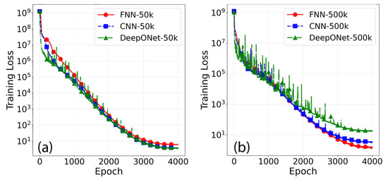
Figure 7. Homoscedastic uncertainty weighted training loss (log scale) for FNN, CNN, and DeepONet: (a) 50k parameters and (b) 500k parameters.

As for the components of the homoscedastic uncertainty weighted loss (Equations (11) and (12)), Figure 8 shows the training errors (MSE for $\mathit{P}\left(t_0\right)$, $\mathit{P}\left(t_{peak}\right)$, and $\mathsf{\Delta }t$) for the 50k and 500k models. All models reach low error values; for instance, the largest pressure MSE among the 50k/500k models is $\approx 4.5\times {10}^5 {\mathrm{P}\mathrm{a}}^2$, implying a small Root-MSE (RSME) of $\approx 670 \mathrm{P}\mathrm{a}$. For context, a $1000 \mathrm{P}\mathrm{a}$ hydrostatic pressure corresponds to a depth of 0.10 m. For rise time $\mathsf{\Delta }t$, the largest MSE is only $\approx 2.0\times {10}^{-2} {\mathrm{s}}^2$ $(RMSE \approx 0.14 \mathrm{s}).$ Additionally, scaling model sizes from 50k to 500k improves the pressure prediction performance for FNN and CNN, reduces it for DeepONet, and slightly worsens wave rise time prediction for all models (errors remain low).

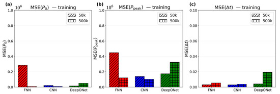
Figure 8. Training MSE for (a) $\mathit{P}\left(t_0\right)$, (b) $\mathit{P}\left(t_{peak}\right)$, and (c) $\mathsf{\Delta }t$ across FNN (red), CNN (blue), and DeepONet (green), each with 50k and 500k parameters.

As for wave rise time $\mathsf{\Delta }t$ prediction performance, parity scatter plots (predicted vs. ground-truth $\mathsf{\Delta }t$) for the 50k and 500k model sizes for the 100-sample training set are shown in Figure 9. Across all models (FNN, CNN, and DeepONet), both sizes predict $\mathsf{\Delta }t$ well, where all coefficients of determination are $R^2$≥ 0.98. This might imply that homoscedastic uncertainty loss (Equation (10)) succeeded in preventing $\mathsf{\Delta }t$, due to its small scale, from being ignored during training. Section 3.6 discusses training the models with equal weight losses for pressures and wave rise time to assess the impact of homoscedastic uncertainty weighting.

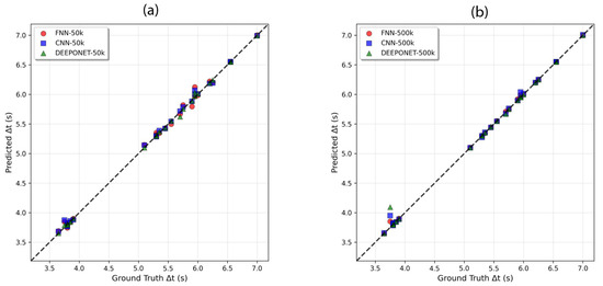
Figure 9. Parity scatter plots of predicted vs. ground-truth rise time $\mathsf{\Delta }t$ for (a) 50k models and (b) 500k models. Dashed line denotes perfect agreement.

For a closer examination, Figure 10 (50k models) and Figure 11 (500k models) present a training sample {$R_n=0.5$, $d_r=3.75 \mathrm{m}, H=2.4 \mathrm{m}$} showing (a) ground-truth and output predictions for pressure maps and wave wise time $\left\{\mathit{P}\right(t_0)$, $\mathit{P}\left(t_{peak}\right),$ $\mathsf{\Delta }t$} and (b) absolute error of pressure maps at $t_0$ and $t_{peak}$ for FNN, CNN, and DeepONet. All three architectures, with 50k and 500k sizes, capture $\mathit{P}\left(t_0\right)$, almost perfectly. Although small, the $\mathit{P}\left(t_0\right)$ error horizontal band in FNN-50k (Figure 10b) disappears in FNN-500k (Figure 11b), and this is consistent with the earlier observation that FNN benefits most from scaling out of all three architectures considered. For $\mathit{P}\left(t_{peak}\right)$, performance remains good for all models, where maximum absolute error is $~6000 \mathrm{P}\mathrm{a}$ (occurring above the SWL), with the 500k models exhibiting slightly lower error spread.

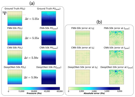
Figure 10. Representative training sample {$R_n=0.5$, $d_r=3.75 \mathrm{m}, H=2.4 \mathrm{m}$} (a) ground-truth and predicted pressure maps $\left\{\mathit{P}\right(t_0)$, $\mathit{P}\left(t_{peak}\right)\}$ and wave rise time $\mathsf{\Delta }t$; (b) error pressure maps at $t_0$ and $t_{peak}$ for 50k parameters models.

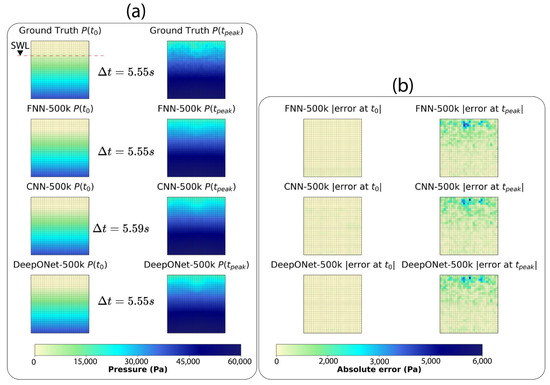
Figure 11. Representative training sample {$R_n=0.5$, $d_r=3.75 \mathrm{m}, H=2.4 \mathrm{m}$} (a) ground-truth and predicted pressure maps $\left\{\mathit{P}\right(t_0)$, $\mathit{P}\left(t_{peak}\right)\}$ and wave rise time $\mathsf{\Delta }t$; (b) error pressure maps at $t_0$ and $t_{peak}$ for 500k parameters models.

3.4. Performance on Testing Set

Testing is conducted on 25 held-out samples (20%) to assess generalization of the models. Figure 8 reports training results, and Figure 12 reports testing results. The following important observations are thus made. Pressure map errors are low across all models (max $RMSE \approx 600 \mathrm{P}\mathrm{a}$). All models capture $\mathit{P}\left(t_0\right)$ well, with FNN-50k showing the maximum $RMSE \approx 550 \mathrm{P}\mathrm{a}$. Additionally, testing MSE (Figure 12) closely matches training set MSE (Figure 8), indicating good generalization within the operating data range of FSBWs in Table 1. Unlike the training results, scaling the models’ sizes improves pressure map {$\left\{\mathit{P}\right(t_0)$, $\mathit{P}\left(t_{peak}\right)\}$ accuracy on the testing set, with all 500k models showing lower MSEs than their 50k counterparts (Figure 12a,b). However, this trend does not hold for wave rise time (Figure 12c). Given the low test MSE, the 50k models are acceptable and scaling to 500k provides improvement but is not necessary. The next section evaluates a compact 5k parameter model (1/10th of 50k) to examine the effect of substantial reduction in number of parameters.

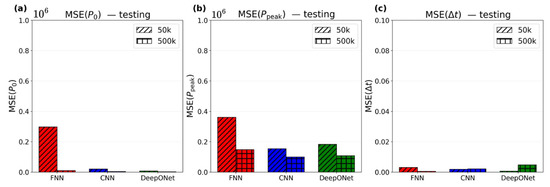
Figure 12. Testing MSE for (a) $\mathit{P}\left(t_0\right)$, (b) $\mathit{P}\left(t_{peak}\right)$, and (c) $\mathsf{\Delta }t$ across FNN (red), CNN (blue), and DeepONet (green), each with 50k and 500k parameters.

3.5. Compact Models

As shown in the previous section, the 50k parameter models are a practical choice; though scaling to 500k results in improvements in testing set pressure predictions, 50k models’ errors are already small. In contrast, substantially reducing the parameter count reduces accuracy. To illustrate this, 5k (1/10th of the 50k) variants of the FNN, CNN, and DeepONet are trained, with the same settings shown in Table 3. The test set MSE of the 5k models alongside the 50k and 500k counterparts are shown in Figure 13.

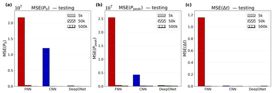
Figure 13. Testing MSE for (a) $\mathit{P}\left(t_0\right)$, (b) $\mathit{P}\left(t_{peak}\right)$, and (c) $\mathsf{\Delta }t$ across FNN (red), CNN (blue), and DeepONet (green), each with 5k, 50k, and 500k parameters.

As shown in Figure 13, testing set pressure MSE for the 5k models are substantially higher than those for the 50k and 500k variants across all three architectures. For FNN and CNN, the $\mathit{P}\left(t_0\right)$ MSE increases by $>2000$, relative to the 500k counterparts, and the $\mathit{P}\left(t_{peak}\right)$ MSE by $>40$. In contrast, the effect of downsizing to 5k is less pronounced for DeepONet (~80x for $\mathit{P}\left(t_0\right)$ and ~3x for $\mathit{P}\left(t_{peak}\right)$, compared to the 500k counterpart). Hence, if a compact model is required, DeepONet is the most robust under aggressive parameter reduction.

3.6. Loss Function Variation

In this study, the homoscedastic uncertainty weighting function Equation (10) is initially adopted to avoid manual loss weight tuning [50] when jointly learning two targets (pressure and wave rise time) with different scales. However, because the architectures in Figure 3 include a dedicated MLP head for $\mathsf{\Delta }t$ (i.e., the target with small scale), it is not clear whether homoscedastic uncertainty weighting is necessary. To assess this, this section uses an equal weights loss defined as follows:

$$\mathcal{L}=w_1{L}_{\mathit{P}}+{w_{2}L}_{\mathsf{\Delta }t}$$

(13)

Here, $w_1=w_2=1$, and $L_{\mathit{P}}$ and $L_{\mathsf{\Delta }}$ are defined in Equations (11) and (12), respectively.

The 50k and 500k models are retrained with this loss function, and all other training settings remain unchanged (see Table 3) with test metric $R^2$ for $\mathsf{\Delta }t$ shown in Figure 14. For both model sizes FNN and CNN, the equal weighting loss yields excellent results, with $R^2\ge 0.97$. For the DeepONet, the 50k model shows a slight improvement under equal weighting ($R^2=0.99$) compared to the homoscedastic loss ($R^2=0.97$). However, for the 500k model, the improvement using equal weights loss is more pronounced compared to the homoscedastic loss ($R^2=0.89$ vs. $R^2=0.81$).

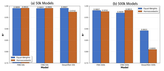
Figure 14. Coefficient of determination $R^2$ for wave rise time $\mathsf{\Delta }t$ test performance: equal weights vs. homoscedastic loss functions for (a) 50k and (b) 500k parameter models.

Overall, the results suggest that the dedicated MLP head for $\mathsf{\Delta }t$ (Figure 3) enables accurate wave rise time prediction without explicit homoscedastic uncertainty weighting. Nevertheless, homoscedastic weighting remains a sound default in multitask settings where the targets have different scales [50] and provides improvements in most cases (CNN and FNN) while deteriorating performance in others (DeepONet), as can be seen in Figure 14.

4. Summary and Conclusions

This study develops an SPH-ANN workflow to predict wave pressures on a hypar FSBW. A dataset of 125 SPH simulations is assembled using the inputs, hypar normalized rise $R_n$ breakwater draft $d_r$, and solitary wave height $H$. The targets are two 30 × 30 hypar surface pressure maps at wave arrival (hydrostatic) and at peak sum of pressures, $\left\{\mathit{P}\right(t_0)$, $\mathit{P}\left(t_{peak}\right)$}, and the wave rise time $\mathsf{\Delta }t=t_{peak}-t_0$. Three architectures (FNN, CNN, DeepONet) are trained with ~50k and ~500k parameters. The models are trained on 100 samples and evaluated on 25 held-out samples. Inference for each new sample requires less than 2 milliseconds. The following conclusions are drawn:

The workflow produces models that generalize well across the FSBW operating range. Testing errors are low across architectures and both 50k and 500k sizes, with training and testing errors closely matching.

The 50k parameter models are sufficient, while 500k yields some improvements in pressure map prediction. Further reducing to 5k reduces accuracy as follows: DeepONet is most robust under substantial parameter reduction (500k to 5k), whereas FNN and CNN performance largely degrade. FNN is found to benefit the most from scaling up model size.

A single neural network can jointly predict pressure maps and wave rise time, even though the targets are on different scales. Homoscedastic uncertainty weighting is found to provide a slight improvement for $\mathsf{\Delta }t$ predictions in most CNN and FNN models and deteriorates the performance for DeepONet models. Overall, homoscedastic loss is found to be unnecessary as $\mathsf{\Delta }t$ has a dedicated MLP head in all models.

Inference using the trained models takes less than 2 milliseconds, providing a substantial speedup compared to running new SPH simulations.

Although the study presents a novel contribution, its limitations include consideration of only solitary waves, a fixed geometry (with varying warping), and prediction of just two pressure maps at different time steps. The dataset’s small size, while sufficient for demonstrating good generalization within the considered operating parameter space (Table 1), may limit the model’s ability to extrapolate to a wider range of geometric and wave conditions. Future work could extend to regular and irregular waves, the prediction of full pressure map time history (via sequence modeling), varying geometric dimensions, and the incorporation of physics-informed components in the loss function. Finally, it is important to note that the ANN models developed in this study inherit the accuracy and limitations of the underlying SPH data; therefore, a broader experimental program for hypar FSBWs over a wider range of parameters with direct pressure measurements would be highly valuable.

References

- Vardy, M.; Oppenheimer, M.; Dubash, N.K.; O’Reilly, J.; Jamieson, D. The intergovernmental panel on climate change: Challenges and opportunities. Annu. Rev. Environ. Resour. 2017, 42, 55–75. [Google Scholar] [CrossRef]
- Rambabu, N.; Srineash, V.K. A Review on Methodologies to Upgrade the Coastal Structures to Enhance the Coastal Resilience. In Proceedings of the OCEANS 2022—Chennai, Chennai, India, 21–24 February 2022; IEEE: Piscataway, NJ, USA, 2022; pp. 1–9. [Google Scholar] [CrossRef]
- Pérez-Alarcón, A.; Fernández-Alvarez, J.C.; Coll-Hidalgo, P. Global increase of the intensity of tropical cyclones under global warming based on their maximum potential intensity and CMIP6 models. Environ. Process. 2023, 10, 36. [Google Scholar] [CrossRef]
- Dai, J.; Wang, C.M.; Utsunomiya, T.; Duan, W. Review of recent research and developments on floating breakwaters. Ocean. Eng. 2018, 158, 132–151. [Google Scholar] [CrossRef]
- Vicinanza, D.; Lauro, E.D.; Contestabile, P.; Gisonni, C.; Lara, J.L.; Losada, I.J. Review of Innovative Harbor Breakwaters for Wave-Energy Conversion. J. Waterw. Port Coast. Ocean. Eng. 2019, 145, 03119001. [Google Scholar] [CrossRef]
- Calheiros-Cabral, T.; Rosa-Santos, P.; Taveira-Pinto, F.; Lara, J.L. Harnessing wave energy through breakwater integration: A review of technologies, deployment strategies and an open-access database. Renew. Sustain. Energy Rev. 2025, 223, 115975. [Google Scholar] [CrossRef]
- Teh, H. Hydraulic performance of free surface breakwaters: A review. Sains Malays. 2013, 42, 1301–1310. [Google Scholar]
- Isaacson, M.; Whiteside, N.; Gardiner, R.; Hay, D. Modelling of a circular-section floating breakwater. Can. J. Civ. Eng. 1995, 22, 714–722. [Google Scholar] [CrossRef]
- Ghassemizadeh, S.; ShojaeeBaghdar, F.; Mazaherizaveh, A.; BaghdarShojaee, R.; Ghasemizadeh, A.; Talesh-Alikhani, E. A Comparative Numerical Study of Solitary Wave Interaction with Concave, Convex, and Sloped Seawalls: Hydrodynamics, Wave Loads, and Turbulent Flow Analysis. Res. Sq. 2025. [Google Scholar] [CrossRef]
- Turkyilmazoglu, M. Maximum wave run-up over beaches of convex/concave bottom profiles. Cont. Shelf Res. 2022, 232, 104610. [Google Scholar] [CrossRef]
- Wu, G.; Smith, S.; Pawitan, K.A.; Garlock, M. An SPH study of cross-sectional shape effects on coastal structures subject to regular wave forces. Ocean. Eng. 2025, 342, 122929. [Google Scholar] [CrossRef]
- ElDarwich, H.S.; Pawitan, K.A.; Garlock, M.E. Conceptual investigation on the effectiveness of hyperbolic paraboloid surfaces for floating breakwaters. In Proceedings of the IASS 2022 Symposium Affiliated with APCS 2022 Conference, Online & Beijing Friendship Hotel, Beijing, China, 19–23 September 2022, ISSN 2518-6582. [Google Scholar]
- ElDarwich, H.; Pawitan, K.A.; Garlock, M. Investigation of Hyperbolic Paraboloid Face Profile Efficacy for Free-Surface Breakwaters. Coast. Eng. Proc. 2024, 38, 67. [Google Scholar] [CrossRef]
- Liu, Z.; Wang, Y. Numerical studies of submerged moored box-type floating breakwaters with different shapes of cross-sections using SPH. Coast. Eng. 2020, 158, 103687. [Google Scholar] [CrossRef]
- Panda, A.; Muduli, R.; Karmakar, D.; Rao, M. Hydrodynamic performance of H-shaped floating breakwater in the presence of a partially reflecting seawall. Mar. Georesources Geotechnol. 2025, 1–31. [Google Scholar] [CrossRef]
- Günaydın, K.; Kabdaşlı, M. Performance of solid and perforated U-type breakwaters under regular and irregular waves. Ocean. Eng. 2004, 31, 1377–1405. [Google Scholar] [CrossRef]
- Wang, Y.; Wang, G.; Li, G. Experimental study on the performance of the multiple-layer breakwater. Ocean. Eng. 2006, 33, 1829–1839. [Google Scholar] [CrossRef]
- Sundar, V. Hydrodynamic pressures and forces on quadrant front face pile supported breakwater. Ocean. Eng. 2002, 29, 193–214. [Google Scholar] [CrossRef]
- Koutandos, E.; Prinos, P. Hydrodynamic characteristics of semi-immersed breakwater with an attached porous plate. Ocean. Eng. 2011, 38, 34–48. [Google Scholar] [CrossRef]
- Smith, S.; Wu, G.; Pawitan, K.; Garlock, M. Hyperbolic Paraboloid Free-Surface Breakwaters: Hydrodynamic Study and Structural Evaluation. J. Mar. Sci. Eng. 2025, 13, 245. [Google Scholar] [CrossRef]
- Elchahal, G.; Lafon, P.; Younes, R. Design optimization of floating breakwaters with an interdisciplinary fluid–solid structural problem. Can. J. Civ. Eng. 2009, 36, 1732–1743. [Google Scholar] [CrossRef]
- Cebada-Relea, A.J.; López, M.; Claus, R.; Aenlle, M. Short-term analysis of extreme wave-induced forces on the connections of a floating breakwater. Ocean. Eng. 2023, 280, 114579. [Google Scholar] [CrossRef]
- Smith, S.; Mansouri, I.; Garlock, M.; Wang, S. Predicting maximum deflection of N-Edged thin-shelled hyperbolic-Paraboloid umbrella using machine learning techniques. Thin-Walled Struct. 2024, 205, 112412. [Google Scholar] [CrossRef]
- Garlock, M.E.M.; Billington, D.P. Félix Candela: Engineer, Builder, Structural Artist; Princeton University Art Museum: Princeton, NJ, USA; Yale University Press: New Haven, CT, USA, 2008. [Google Scholar]
- Billington, D.P. Thin Shell Concrete Structures; McGraw-Hill: New York, NY, USA, 1965. [Google Scholar]
- Gergely, P.; Banavalkar, P.V.; Parker, J.E. The Analysis and Behavior of Thin-Steel Hyperbolic Paraboloid Shells. 1971. Available online: https://scholarsmine.mst.edu/ccfss-library/19/ (accessed on 12 December 2023).
- Wang, S.; Garlock, M.; Deike, L.; Glisic, B. Feasibility of Kinetic Umbrellas as deployable flood barriers during landfalling hurricanes. J. Struct. Eng. 2022, 148, 04022047. [Google Scholar] [CrossRef]
- Wu, G.; Garlock, M.; Wang, S. A decoupled SPH-FEM analysis of hydrodynamic wave pressure on hyperbolic-paraboloid thin-shell coastal armor and corresponding structural response. Eng. Struct. 2022, 268, 114738. [Google Scholar] [CrossRef]
- Crespo, A.J.; Domínguez, J.M.; Rogers, B.D.; Gómez-Gesteira, M.; Longshaw, S.; Canelas, R.; Vacondio, R.; Barreiro, A.; García-Feal, O. DualSPHysics: Open-source parallel CFD solver based on Smoothed Particle Hydrodynamics (SPH). Comput. Phys. Commun. 2015, 187, 204–216. [Google Scholar] [CrossRef]
- Monaghan, J.J. Smoothed particle hydrodynamics. Rep. Prog. Phys. 2005, 68, 1703. [Google Scholar] [CrossRef]
- Altomare, C.; Domínguez, J.M.; Crespo, A.J.C.; González-Cao, J.; Suzuki, T.; Gómez-Gesteira, M.; Troch, P. Long-crested wave generation and absorption for SPH-based DualSPHysics model. Coast. Eng. 2017, 127, 37–54. [Google Scholar] [CrossRef]
- Abouhalima, M.; Das Neves, L.; Taveira-Pinto, F.; Rosa-Santos, P. Machine Learning in Coastal Engineering: Applications, Challenges, and Perspectives. J. Mar. Sci. Eng. 2024, 12, 638. [Google Scholar] [CrossRef]
- Zanuttigh, B.; Formentin, S.M.; Briganti, R. A neural network for the prediction of wave reflection from coastal and harbor structures. Coast. Eng. 2013, 80, 49–67. [Google Scholar] [CrossRef]
- Kuntoji, G.; Rao, S.; Manu. Prediction of Wave Transmission over an Outer Submerged Reef of Tandem Breakwater Using RBF-Based Support Vector Regression Technique. In Proceedings of the Fourth International Conference in Ocean Engineering (ICOE2018), Chennai, India, 18–21 February 2018; Murali, K., Sriram, V., Samad, A., Saha, N., Eds.; Springer: Singapore, 2019; Volume 23, pp. 559–570. [Google Scholar] [CrossRef]
- Van Gent, M.R.A.; Van Den Boogaard, H.F.P.; Pozueta, B.; Medina, J.R. Neural network modelling of wave overtopping at coastal structures. Coast. Eng. 2007, 54, 586–593. [Google Scholar] [CrossRef]
- Antoci, C.; Gallati, M.; Sibilla, S. Numerical simulation of fluid–structure interaction by SPH. Comput. Struct. 2007, 85, 879–890. [Google Scholar] [CrossRef]
- Hornik, K. Approximation capabilities of multilayer feedforward networks. Neural Netw. 1991, 4, 251–257. [Google Scholar] [CrossRef]
- Lecun, Y.; Bottou, L.; Bengio, Y.; Haffner, P. Gradient-based learning applied to document recognition. Proc. IEEE 1998, 86, 2278–2324. [Google Scholar] [CrossRef]
- Lu, L.; Jin, P.; Pang, G.; Zhang, Z.; Karniadakis, G.E. Learning nonlinear operators via DeepONet based on the universal approximation theorem of operators. Nat. Mach. Intell. 2021, 3, 218–229. [Google Scholar] [CrossRef]
- Wendland, H. Piecewise polynomial, positive definite and compactly supported radial functions of minimal degree. Adv. Comput. Math. 1995, 4, 389–396. [Google Scholar] [CrossRef]
- Fourtakas, G.; Vacondio, R.; Alonso, J.D.; Rogers, B.D. Improved density diffusion term for long duration wave propagation. In Proceedings of the 2020 SPHERIC Harbin International Workshop, Harbin, China, 13 January–16 September 2020. [Google Scholar]
- Batchelor, G.K. An Introduction to Fluid Dynamics, 1st ed.; Cambridge University Press: Cambridge, UK, 2000. [Google Scholar] [CrossRef]
- Estevez, I.M. Coupling Between the DualSPHysics Solver and Multiphysics Libraries: Implementation, Validation and Real Engineering Applications. Ph.D. Thesis, Universidade de Vigo, Pontevedra, Spain, 2024. [Google Scholar]
- Wang, S.; Notario, V.; Garlock, M.; Glisic, B. Parameterization of hydrostatic behavior of deployable hypar umbrellas as flood barriers. Thin-Walled Struct. 2021, 163, 107650. [Google Scholar] [CrossRef]
- Cabrera Crespo, A.J.; Gómez Gesteira, R.; Dalrymple, R.A. Boundary conditions generated by dynamic particles in SPH methods. Comput. Mater. Contin. 2007, 5, 173. [Google Scholar]
- Goring, D.G.; Raichlen, F. Tsunamis, the Propagation of Long Waves onto a Shelf; California Institute of Technology: Pasadena, CA, USA, 1978. [Google Scholar]
- McNeel. Rhinoceros 3D, Version 7; McNeel: Seattle, WA, USA, 2015. [Google Scholar]
- Butterworth, S. On the theory of filter amplifiers. Wirel. Eng. 1930, 7, 536–541. [Google Scholar]
- Ko, H.T.-S.; Cox, D.T.; Riggs, H.R.; Naito, C.J. Hydraulic Experiments on Impact Forces from Tsunami-Driven Debris. J. Waterw. Port Coast. Ocean. Eng. 2015, 141, 04014043. [Google Scholar] [CrossRef]
- Kendall, A.; Gal, Y.; Cipolla, R. Multi-task learning using uncertainty to weigh losses for scene geometry and semantics. In Proceedings of the IEEE Conference on Computer Vision and Pattern Recognition (CVPR), Salt Lake City, UT, USA, 18–22 June 2018; pp. 7482–7491. [Google Scholar]
- Kingma, D.P.; Ba, J. Adam: A Method for Stochastic Optimization. arXiv 2014. [Google Scholar] [CrossRef]
- He, K.; Zhang, X.; Ren, S.; Sun, J. Delving Deep into Rectifiers: Surpassing Human-Level Performance on ImageNet Classification. arXiv 2015. [Google Scholar] [CrossRef]
- Hendrycks, D.; Gimpel, K. Gaussian Error Linear Units (GELUs). arXiv 2016. [Google Scholar] [CrossRef]
- Fisher, R.A. The Arrangement of Field Experiments. In Breakthroughs in Statistics; Kotz, S., Johnson, N.L., Eds.; Springer: New York, NY, USA, 1992; pp. 82–91. [Google Scholar] [CrossRef]
- Cybenko, G. Approximation by superpositions of a sigmoidal function. Math. Control. Signals Syst. 1989, 2, 303–314. [Google Scholar] [CrossRef]
- Qian, G.; Li, Y.; Peng, H.; Mai, J.; Hammoud, H.; Elhoseiny, M.; Ghanem, B. Pointnext: Revisiting pointnet++ with improved training and scaling strategies. Adv. Neural Inf. Process. Syst. 2022, 35, 23192–23204. [Google Scholar]
- Loshchilov, I.; Hutter, F. SGDR: Stochastic Gradient Descent with Warm Restarts. arXiv 2016. [Google Scholar] [CrossRef]
Disclaimer/Publisher’s Note: The statements, opinions and data contained in all publications are solely those of the individual author(s) and contributor(s) and not of MDPI and/or the editor(s). MDPI and/or the editor(s) disclaim responsibility for any injury to people or property resulting from any ideas, methods, instructions or products referred to in the content. |
© 2025 by the authors. Licensee MDPI, Basel, Switzerland. This article is an open access article distributed under the terms and conditions of the Creative Commons Attribution (CC BY) license (https://creativecommons.org/licenses/by/4.0/).