Abstract
This study focuses on an integrated three-level multi-port liner ship vessel routing and scheduling optimization problem. Specifically, the three-level multi-port network consists of hub ports, feeder ports, and cargo source points, which provide the demands’ loading/unloading at each port. Considering vessel-specific constraints such as speed, capacity, and cost, we formulate the multi-port liner ship routing and scheduling optimization problem as a mixed integer linear programming model with the objective of minimizing total voyage cost and operating time. First, we employ machine learning models to forecast the short-term demand at different ports as the input. There are multiple feasible routes generated and allowed to be elected. Second, to ensure both computational efficiency and solution quality, we devise and compare genetic algorithm (GA), simulated annealing (SA), Gurobi and the branch-and-price (B&P) algorithm to optimize scheduling plans. Experimental results demonstrate that the proposed predict-then-optimization framework effectively addresses the complexity of multi-port scheduling and routing problems, achieving a reduction in total transportation cost by 0.81% to 8.08% and a decrease in computation time by 16.86% to 24.7% compared to baseline methods, particularly with the SA + B&P hybrid approach. This leads to overall efficiency and cost-saving ocean vessel operations.
1. Introduction
The optimization of multi-port routes for ocean-going vessels is a critical issue in maritime logistics, directly affecting transportation efficiency, operational costs, and service quality. With the continuous growth of global trade, the complexity and difficulty of vessel scheduling have significantly increased. Traditional scheduling methods often encounter challenges in effectively addressing dynamic factors such as fluctuating port handling demands, vessel speed adjustments, and fuel consumption variations. Thus, it enlightens us to develop an integrated framework combining advanced forecasting models and optimization algorithms.
This study proposes and develops a comprehensive scheduling optimization framework that integrates demand forecasting with B&P for multi-port liner shipping. The framework constructs a port network comprising hub ports, feeder ports, and cargo origin points based on port classification generation models. Using a Long Short-Term Memory (LSTM) deep learning model, it accurately forecasts the loading and unloading demand at each port, thereby capturing the dynamic characteristics of market demand. Considering various vessel types’ sailing speeds, capacities, and cost parameters, the framework generates multiple feasible routes and employs GA, SA, and the B&P alongside the commercial solver Gurobi to optimize vessel scheduling with the objective of minimizing total route cost and transit time.
Furthermore, the framework incorporates a feeder vessel simulation module to model the transshipment strategies between cargo origin points and feeder ports, better reflecting real-world transportation scenarios. This study accounts for dynamic fuel consumption models and the impact of vessel speed variations on operational costs, balancing fuel expenses and sailing time to improve overall economic efficiency. To enhance the system’s practicality and analytical capabilities, a comprehensive result analysis and visualization module has been developed, enabling comparative evaluation of optimal solutions under different numbers of port calls.
Extensive experimental results demonstrate that the proposed system significantly outperforms in handling the complexity of multi-port vessel scheduling. The LSTM-based demand forecasting markedly improves the accuracy of handling volume predictions, enabling more realistic and efficient scheduling plans that reduce resource waste and delay risks. The dynamic fuel consumption model facilitates reasonable speed adjustments, cutting fuel costs. By devising a B&P algorithm, the framework achieves dual objectives of cost and time minimization. The framework exhibits strong adaptability across multiple test datasets, confirming its feasibility and superiority.
In summary, this study not only offers a new approach to multi-port ocean vessel scheduling but also provides algorithmic support for shipping companies to enhance transportation efficiency and reduce operational costs, holding significant theoretical value and practical application prospects.
2. Literature Review
This study proposes a framework that integrates “three-level network dynamic modeling-LSTM demand forecasting-SA + B&P hybrid algorithm” for the multi-port liner scheduling optimization problem. Its cutting-edge and scientific nature are highlighted through systematic literature comparison. In terms of network modeling, Yue and Mangan [1] adopted a static reliability framework and focused on network topology analysis but did not involve dynamic scheduling constraints, resulting in insufficient adaptability of the model in actual operations. Xu et al. [2] described the global port correlation through multiple network theory, providing structural insights, but lacked integration with optimization algorithms and could not handle real-time scheduling problems. Li et al. [3] developed a robust routing solution to deal with weather uncertainty and introduced a network redundancy strategy, but the model assumed a flat network and did not distinguish between trunk and branch functions, which limited the efficiency of multi-port collaboration. Dos Santos and Borenstein [4] constructed a multi-objective optimization framework to balance cost and time objectives but simplified the network structure and ignored the hierarchical division of labor, which may cause resource allocation conflicts in actual applications. Zhao et al. [5] used GA for roll-on/roll-off transport scheduling, achieving a cost saving of about 5%, but the network model assumed that all ports were directly accessible, which was disconnected from the hub-feeder hierarchy in real logistics; Asnicar et al. [6] reviewed the application of machine learning in the scientific field, which provided cross-disciplinary insights but was not directly applied to shipping network optimization. Yang et al. [7] analyzed the emission characteristics of ships through field measurements, emphasizing environmental factors, but did not combine them with network modeling. Wang et al. [8] studied hybrid power and the waste heat recovery of power ships focusing on energy efficiency, but the scope is limited to the power system and has not been extended to the scheduling network. Zhao et al. [9] optimized the ore transportation sailing plan and handled specific cargo types, but the network model was single and lacked universality. Elmi et al. [10] developed a linear scheduling recovery model based on the ε constraint method, emphasizing real-time adjustment but did not consider the multi-level network structure. Du et al. [11] integrated the shipper selection behavior into the container scheduling, adding a behavioral economics dimension, but the network structure was simple and did not handle dynamic demand. Sun et al. [12] designed an accurate algorithm to optimize the quay crane scheduling and improve the port operation efficiency but did not coordinate with the ship routing. Ma et al. [13] developed a multi-ship collaboration framework for offshore wind farms, providing ideas for collaborative scheduling. However, the application areas are quite different from liner shipping and the correlation is weak. He et al. [13] applied the enhanced branch pricing algorithm in production-transportation scheduling, demonstrating the potential of the precise method, but the background is not maritime and does not involve port networks. Chen et al. [14] improved the branch pricing method in machine scheduling, providing a reference for algorithm design but did not deal with network dynamics. Liu et al. [15] studied ship scheduling under sluice coordination and introduced physical constraints, but the model was limited to specific scenarios (such as flood season) and lacked versatility. Zhang et al. [16] explored scheduling under emission restrictions, emphasizing environmental constraints, but the network scope was local and did not cover global optimization. Cai et al. [17] predicted ship fuel consumption based on real data to improve data-driven accuracy, but it is not combined with routing optimization. Wang et al. [18] designed hybrid power system collaborative optimization, focusing on the propulsion system, and did not extend to the scheduling network. Nguyen et al. [19] reviewed the application of artificial intelligence in green shipping, emphasizing sustainability, but lacking specific algorithm implementation; Mahmoodjanloo et al. [20] solved port routing under draft restrictions, introduced physical restrictions but simplified the network model and did not handle multi-level structures. Zhong et al. [21] explored tugboat scheduling under tidal windows, balancing time and environmental goals, but the application scale was small networks. Jin et al. [22] used a prediction model to predict container gate flow, providing port-level demand insights, but did not upgrade to network-level optimization. El Mekkaoui et al. [23] developed a ship arrival time prediction model to enhance operational efficiency, but it was not integrated with scheduling. Nejjarou et al. [24] introduced a hybrid metaheuristic for pipeline scheduling, demonstrating the combination of heuristics and exact methods, but the field was different (manufacturing) and had low relevance to liner scheduling. Ma et al. [25] reiterated the importance of multi-vessel collaboration in offshore wind farms and emphasized the value of collaboration, but the application was limited and irrelevant to liner networks.
In terms of demand forecasting, Tamburini et al. [26] used a column generation method to deal with the optimization of general cargo ship routes, relying on historical data to assume that demand is static, lacking real-time adaptability, resulting in a decrease in the performance of the scheduling scheme in a dynamic environment; Chen et al. [27] developed a robust optimization model to deal with liner alliance scheduling, taking into account sulfur emission restrictions and slot exchanges, but the demand input is a fixed value, and the prediction module is not integrated, which cannot respond to market fluctuations. Song et al. [28] used a gravity-inspired deep learning model to predict global maritime traffic flow, achieving high accuracy (a 15% reduction in traffic flow prediction error), but the prediction results were not closed-loop with the scheduling decision making and were disconnected from the application. Meng et al. [29] analyzed the competitiveness of hub ports through empirical research, providing network-level insights but did not involve dynamic prediction methods. Wang et al. [30] developed a multivariable hybrid system for port throughput volume forecasting, combined with ARIMA and machine learning (LSTM), and achieved an accuracy of MAPE = 7.8%, but the prediction was decoupled from the optimization and was not used for real-time scheduling. Liu et al. [31] used integer programming to optimize port scheduling under weather influences, introduced uncertainty processing, but the scope was limited to port-level operations and was not extended to multi-port networks. Ksciuk et al. [32] reviewed uncertainty in maritime routing and scheduling, identified key challenges (such as weather and demand fluctuations) but did not provide solutions or forecast integration. Golsefidi et al. [33] studied the impact of weather on fuel consumption and reduced emissions by speed optimization, but the forecast module was missing and was not combined with demand dynamics. Omholt-Jensen et al. [34] designed a mathematical heuristic for general cargo ship fuel optimization, achieving a cost saving of about 10%, but the application area was narrow and did not deal with liner demand forecasting. Tirkistanli et al. [35] applied machine learning to predict the ship energy efficiency design index (EEDI), focusing on ship design rather than scheduling needs. In contrast, the LSTM dynamic prediction module in this study improves prediction accuracy to MAPE < 5% (RMSE < 0.1). The latest relevant literature comparisons are shown in Table 1, and the “√” indicate what each document contains in the second to fourth columns of the first row.
Table 1.
Comparison of relevant studies.
3. Contributions and Objectives
To address the complexity of scheduling and routing in container liner shipping systems, this study proposes an integrated optimization framework that closely combines demand forecasting, route planning, and fleet scheduling. Unlike traditional studies that primarily focus on single-vessel routing or assume direct access to all ports, this study adopts a system-level perspective to comprehensively capture the structural and operational intricacies of shipping networks. The main contributions and objectives of this study are as follows:
- (1)
- A three-level transportation network model is structured. The hierarchical network comprising hub ports, feeder ports, and cargo source points is proposed to realistically reflect the coordination between trunk and feeder services in liner shipping operations. Hub ports, as the main nodes of the trunk network, are responsible for handling large-scale cargo collection and distribution. These ports are interconnected via inter-hub trunk lines. Feeder ports, as secondary nodes, collect cargo from nearby origins or distribution centers, and there is also cargo demand between feeder ports, ultimately transporting it to the hub ports. Compared to trunk lines, feeder transport typically involves shorter distances and smaller capacities. Cargo origins, representing the final origin of cargo, are connected only by feeder transport.
- (2)
- The machine learning-based dynamic demand forecasting is executed before optimization. To overcome the limitations of static container throughput assumptions, this study incorporates deep learning techniques—such as Long Short-Term Memory (LSTM) networks—for forecasting dynamic port demand. This enables scheduling optimization to respond to fluctuations in container flows and facilitates demand-driven route planning and capacity matching.
- (3)
- An exact algorithm and heuristics are proposed. The study proposes an exact algorithm (B&P) and heuristic algorithms (GA, SA), and further develops a hybrid approach: heuristics are used to generate high-quality initial route columns, which are then refined by B&P for optimal solutions. This balances solution quality with computational efficiency, particularly for large-scale routing problems.
In summary, this study proposes a comprehensive method to optimize multi-port container liner systems, integrating demand forecasting, route generation, and fleet coordination into a joint framework.
4. Materials and Methods
4.1. Problem Description
As container transportation networks expand and grow more complex, liner shipping systems are evolving into hierarchical structures consisting of hub ports, feeder ports, and cargo origin points. The three-level transportation network model approach emphasizes three different types of port functions. Cargo source points serve as starting points, where cargo is transported to feeder ports via small-scale vessels. This section of the route is feeder transport. Feeder ports are responsible for transporting small batches of cargo from the source. Each feeder port also has transportation needs, and the cargo is ultimately transported to hub ports. Hub Ports serve as the starting and ending points of trunk line transport.
“Scheduling” in this study refers to a comprehensive decision-making process. Against this backdrop, a key challenge is how to effectively coordinate feeder and mainline transport routes to effectively coordinate feeder and trunk shipping routes to meet dynamically changing port demands, allocate time windows for each port visit, loading and unloading times, sailing times and waiting times, and match ship types and capacities to obtain the optimal order for ships to visit ports at the lowest total cost. On one hand, the hierarchical structure’s coordination, path connectivity constraints, and multi-vessel decisions complicate the problem formulation and consequently make the optimization more challenging. On the other hand, port loading and unloading demands exhibit fluctuations in practice, which motivates us to use accurate dynamic demand forecasting method to estimate them. Moreover, scheduling optimization is supposed to simultaneously pursue cost minimization while strictly adhering to practical constraints such as vessel capacity, port operation time windows, and transshipment logistics. This results in a highly complex, large-scale NP-hard problem with a vast solution space.
In this study, the item “scheduling” is defined as a comprehensive decision-making process for a three-level port network (hub port, feed port, and origin point). It aims to collaboratively determine vessel routes, arrival/departure times, loading/unloading task allocation, and vessel configuration while satisfying navigation and port operational constraints. In detail, its objective is to minimize overall navigation costs and operating time. Specifically, scheduling works in the paper include:
- (1)
- Routing decisions: Determining the visiting sequence of each mainline vessel starting from and returning to its hub port (mainline routes) while assigning feeder and cargo-origin routes accordingly.
- (2)
- Timetabling decisions: Determining the estimated arrival and departure times of each vessel at each port, ensuring that the service duration (loading/unloading time) complies with port time windows and
- (3)
- Fuel allocation: Assigning vessel types and capacities to specific routes and determining sailing speeds along each leg to balance fuel consumption and travel time
- (4)
- Feeder connection: Ensuring that feeder vessels arrive at feeder ports before the corresponding mainline vessel , thereby maintaining temporal and capacity synchronization between the feeder and mainline services
- (5)
- Demand-driven coordination: Embedding short-term loading/unloading demand forecasts obtained from the LSTM prediction model into the optimization process for capacity matching and column evaluation.
These decisions are constrained by capacity constraints (Formulas (11) and (12)), time windows and sequence constraints (Formulas (13)–(16)), and the fuel consumption cost function in the objective function. The specific formulas will be shown in detail in Section 4.3.
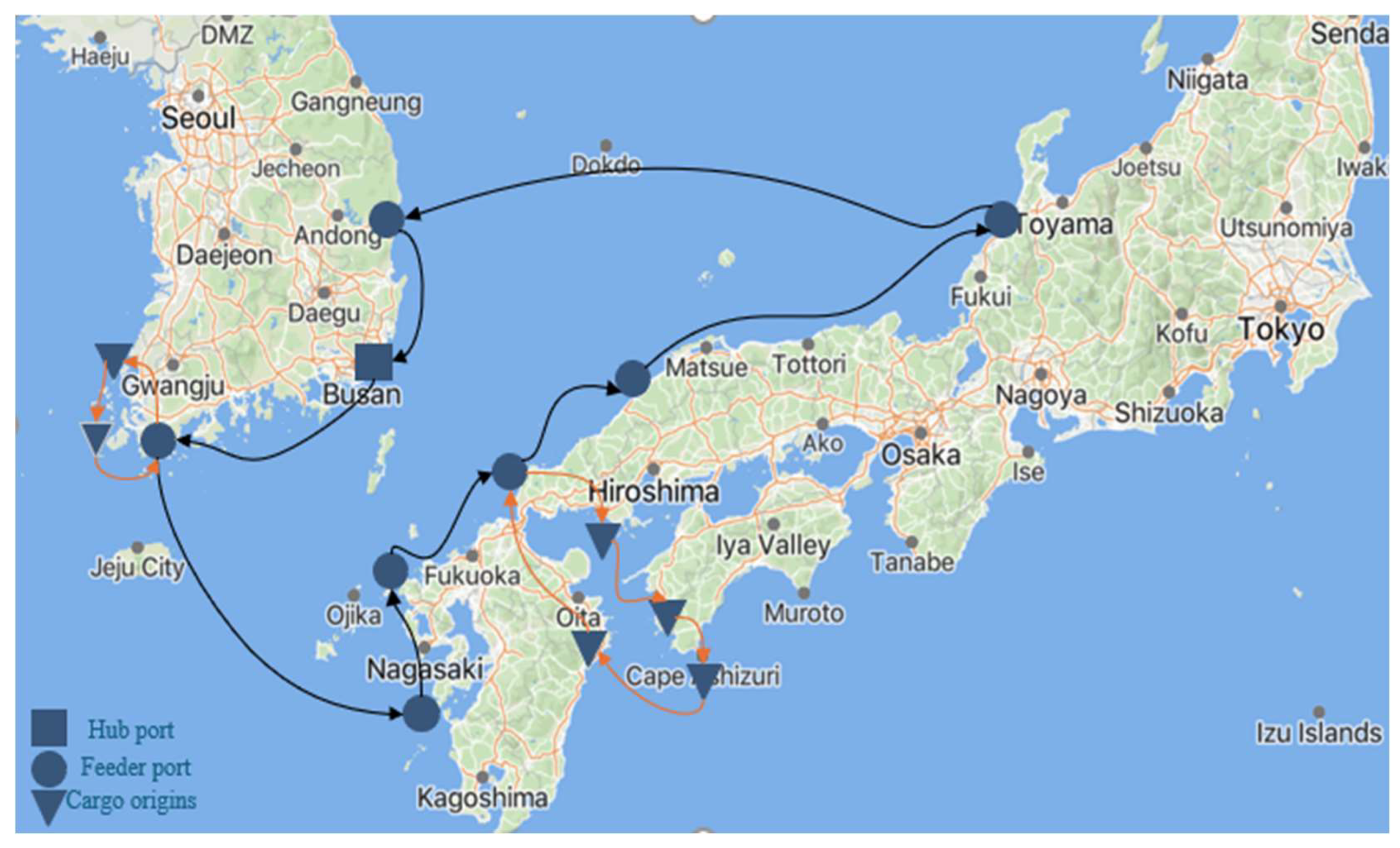
To address these challenges, this paper proposes an integrated scheduling and routing framework that combines machine learning-based demand forecasting, hierarchical network modeling, and hybrid algorithm optimization. The framework not only improves solution accuracy but also significantly enhances computational efficiency in large-scale multi-port systems. The notations of each part of this study are as follows in Table 2. The route diagrammatic drawing of the model is shown in Figure 1, and the black arrows connect the main routes, and the orange arrows connect the feeder routes.
Table 2.
Notations of sets, parameters, and variables.
Figure 1.
Diagram of main and feeder shipping routes.
4.2. Notations
4.3. Model Formulation
We formulate the multi-port container liner shipping optimization model resolving a three-level transportation network problem (comprising hub ports, feeder ports, and cargo origin points). The model captures the coordination between mainline transportation and feeder services. The model aims to minimize total transportation cost while simultaneously obtaining the optimal operational time within the given time window. The total cost includes fixed costs, variable costs (such as fuel consumption), and feeder transportation costs. The cost structure is divided into two main components: the cost of mainline routes and the cost of feeder connections. Fixed costs refer to the inherent operating expenses of various vessel types used on both mainline and feeder routes, as well as container handling charges. Equation (1) represents the objective function for optimizing ship fuel consumption, where denotes the fuel consumption cost, represents the cost of chartering a vessel and is related to the type of vessel chartered and the total duration of the journey, and refers to the environmental emission cost. By minimizing the weighted sum of these three components, the model achieves a balance among fuel economy, transportation efficiency, and environmental benefits. The variable costs are defined by Equation (6), with each component carrying clear operational and economic significance. The complete mathematical formulation of the model is presented in Equation (7). Equation (7) denotes the formulations of the total cost: is the sum of the vessel’s fuel consumption cost, environmental cost, and vessel rental cost; is the cost required for loading and unloading the ship during operation; and is the fixed cost of the ship.
where represents the basic fuel consumption coefficient. represents the power of sailing speed that controls the energy consumption curve (reflecting the sharp increase in fuel consumption at high speeds); represents the multiplicative amplification factor of sea conditions and weather on fuel consumption; represent the weighted coefficient of time and environmental costs, and the environmental impact cost (carbon emissions), respectively. The values of and are not fixed. The value range of is between 0.5–0.7, and the value range of is between 0.3–0.5. The specific corresponding values depend on the scale of scheduling. If it involves complex multi-port cases, the weight of parameter is close to 1.
The constraints are formulated as follows.
Constraint (8) ensures that each vessel departs exclusively from a hub port and eventually returns to the same hub port. Constraint (9) ensures that any vessels entering a feeder port departed from that feeder port. Constraint (10) ensures that each cargo origin point c is assigned to exactly one feeder port. Constraint (11) ensures that the total amount of cargo transported from cargo origin points to ports does not exceed the capacity of vessel. Constraint (12) ensures that, after completing the loading/unloading operations at feeder port i, the remaining capacity of vessel k must be sufficient to meet the loading/unloading demand at the next feeder port j. Constraint (13) ensures that vessel k performs feeder port transport in a sequential order and returns to the hub port before the latest allowable return time. Constraint (14) ensures that vessel k performs feeder port transport sequentially and returns to the hub port before the latest allowable return time. Constraint (15) ensures that the feeder vessel r transports cargo from the origin points to the feeder ports before the main vessel k arrives. Constraint (16) restricts the berthing time of vessel k at feeder port i to lie within the port’s operational time window.
4.4. Algorithm Solution
This section provides a detailed introduction to the implementation processes of three algorithms, i.e., GA, SA and B&P. GA simulates natural selection and genetic mechanisms to iteratively optimize route selection within a population, exhibiting strong global search capabilities and suitability for solving complex combinatorial optimization problems. SA draws inspiration from the physical annealing process, accepting worse solutions with a certain probability to escape local optima and gradually converge to a global optimum, making it particularly effective at avoiding local minima. B&P algorithm is an exact method that systematically partitions the solution space and prunes branches to reduce computational complexity, guaranteeing the discovery of an optimal solution. Finally, a comparative analysis of these three algorithms, alongside the commercial solver Gurobi and their hybrid combinations, will be conducted based on numerical experiments to evaluate their performance differences in solution quality and computational efficiency. Next, we will introduce the algorithm framework used in this study, and focus on how to resolve the model based on the devised algorithms.
4.4.1. Algorithm Framework
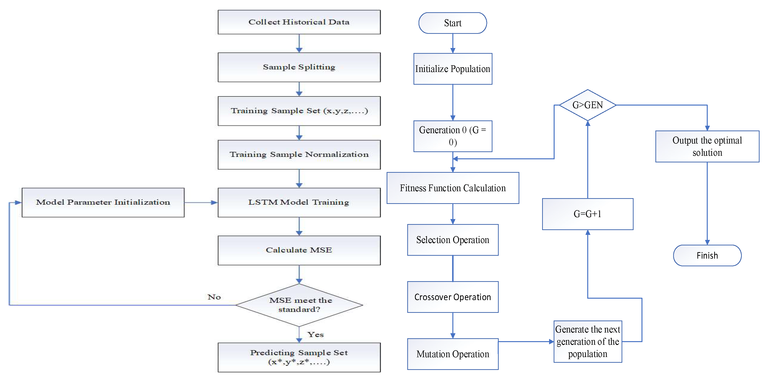
The algorithm framework is a “dynamic demand forecasting and multi-algorithm collaborative optimization” structure. Its objective is to utilize the results predicted by LSTM to input the specific steps in the hybrid algorithm. It first uses LSTM to predict cargo throughput demand at each port, which serves as the mapping input for loading and unloading demand in subsequent algorithms. Then, it first uses Gurobi for computation, and then applies the computed results in a hybrid algorithm. In other words, this is a step-by-step process from dynamic demand forecasting, heuristic algorithms, precise algorithms, and hybrid algorithms. Figure 2 below is a flowchart of GA, LSTM, and B&P.

Figure 2.
Flowchart of GA, LSTM, and B&P.
4.4.2. LSTM Predictions
LSTM prediction aims to handle the uncertainty of port demand in multi-port liner scheduling. We use the LSTM model to predict short-term port demand (loading and unloading volume) and embed the predicted data into the algorithm’s objective function and constraints in real time. The following describes the working process of the LSTM. The main work steps include the following: data preprocessing and input construction, model training and prediction, prediction output, and prediction indicator determination.
The preprocessing layer primarily performs data normalization and seasonal decomposition to reduce the complexity of the time series and thus facilitate the learning process of the subsequent LSTM network. Initially, the time series data is normalized to reduce numerical disparities between different series. A commonly used normalization formula is:
whereis the original value at time t, and and denote the minimum and maximum values of the series, respectively. This min-max scaling maps data to the [0, 1] range, ensuring numerical consistency among features and preventing bias towards variables with larger magnitudes.
Subsequently, seasonal decomposition is a critical step within the preprocessing layer. By separating multiple layers of seasonal patterns, it further reduces the difficulty for the LSTM to learn long sequences. Multi-layer decomposition partitions the time series into three distinct and independent components:
where is the observed value, represents the seasonal component capturing periodic fluctuations, represents the seasonal component capturing periodic fluctuations, denotes the trend component reflecting long-term changes, andis the residual component representing noise and irregular variations. By explicitly isolating these components, the LSTM network can focus on learning the temporal dependencies of the trend and residual parts without being distracted by complex seasonal fluctuations, thus improving prediction accuracy and training efficiency.
The specific workflow is as follows.
Step 1: Input gate.
Controls whether past loading and unloading information is retained at the current point in time. For example, in special circumstances such as the port off-season or the pandemic, old data may be “forgotten”.
Step 2: Forget gate.
Determines how the newly entered historical data (changes in loading and unloading) affects the memory unit. Help capture period-to-period trends in port throughput, seasonal spikes, or sudden congestion.
Step 3: Candidate cell state.
Synthetically forgetting with new inputs, i.e., the first two, updates the current state of need memory.
Step 4: Updated cell state.
Step 5: Output gate.
As an input to the next time step, it is also a characteristic representation of predicting future demand.
Transform the hidden state into the predicted loading and unloading demand of port i at time t + 1. The output results serve as input demand parameters for ports in the scheduling model, directly influencing vessel allocation, route design, and feeder arrangements. They replace the static port demand variables in the original scheduling model, affecting the number of vessels assigned on the main route and the matching of loading capacities.
To evaluate the accuracy and reliability of the demand prediction model, several standard statistical metrics are employed. These metrics quantitatively assess the deviation between the predicted values and the actual values of container throughput at each port. The selected evaluation metrics include:
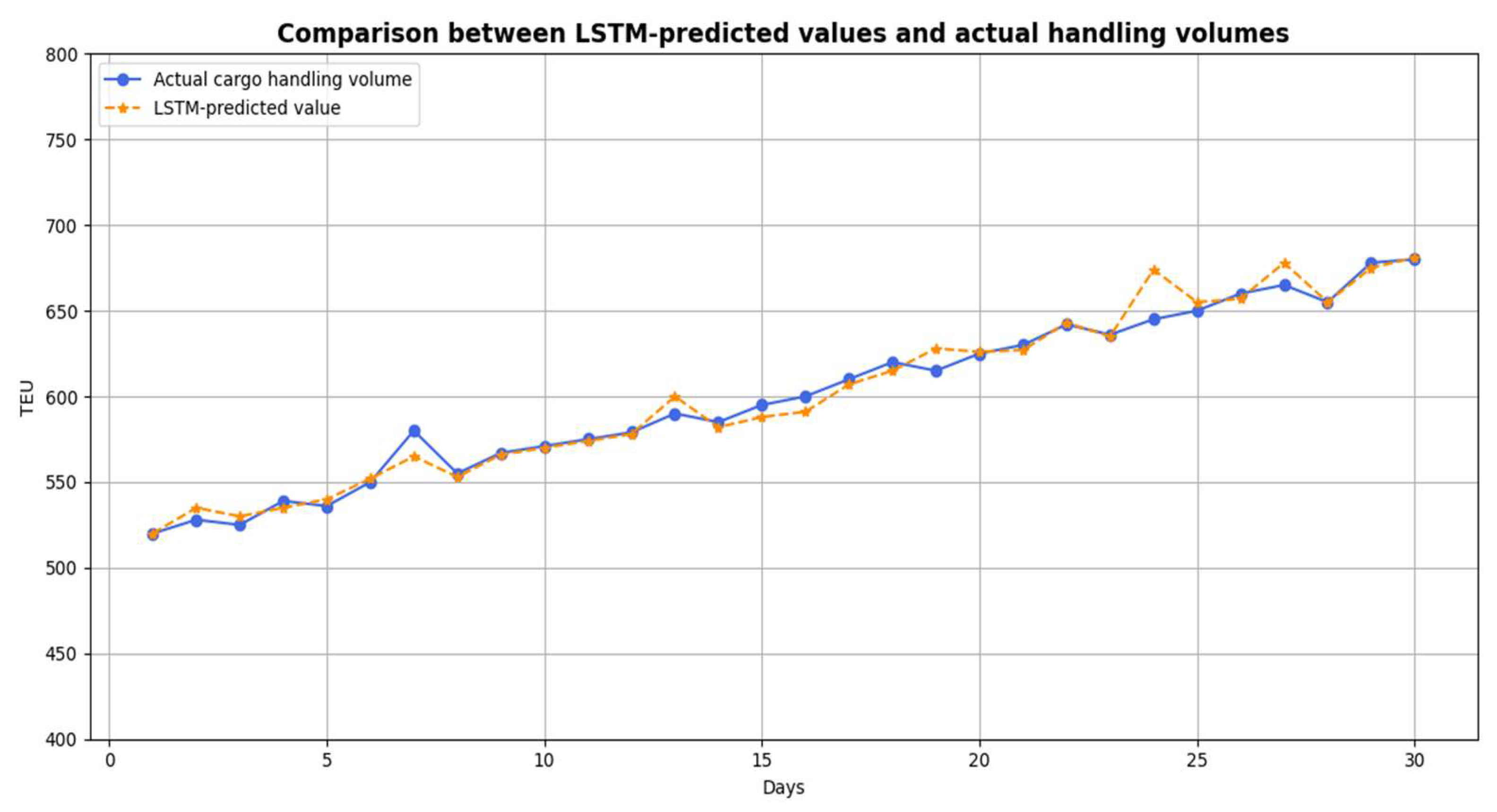
These metrics are calculated on test data sets across multiple port configurations, i.e., small-scale, medium-scale, large-scale networks. The results provide a comprehensive insight into the model’s performance in predicting dynamic container demand, reflecting the LSTM model’s fitting performance on historical samples and its prediction accuracy on future data. This set of metrics reflects the LSTM model’s fit to historical samples and its prediction accuracy for future data, with specific prediction indicators and results presented in Figure 3.
Figure 3.
Forecasting results diagram of 15 ports.
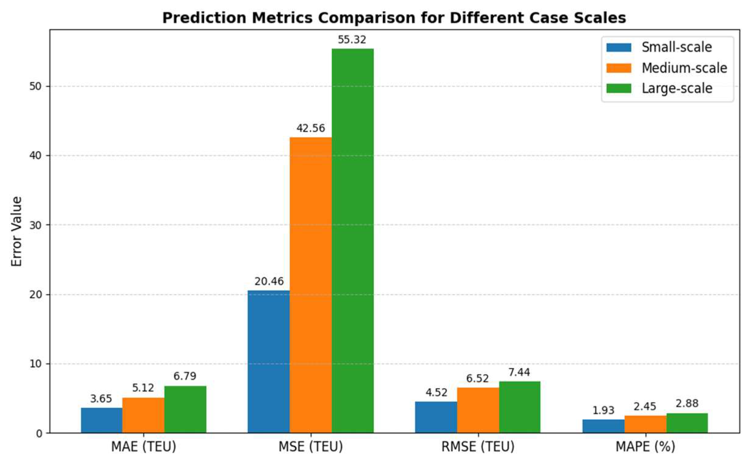
The prediction criteria presented in Figure 4 are obtained by evaluating the predicted values of the three cases.
Figure 4.
Forecasting standard metrics for the three scenarios.
The predicted values obtained by this process ensure that they are consistent with the algorithm, which is specifically accepted by and . The following is the specific process of the algorithm receiving and .
GA receives the predicted value through chromosome encoding, fitness function and genetic operation. The chromosome encoding of GA represents the port visit sequence, with high-demand ports prioritized. In branch routes, cargo source allocation is based on the cargo volume predicted by LSTM, using a “minimum distance first” strategy. The fitness function is defined as the inverse of the total cost. The specific function is:
In the fitness calculation, parameter is affected by , and the new solution generated after crossover and mutation must verify the prediction-related Constraints (11)–(16), ensuring that the ship capacity covers the demand and the arrival time window is set. Individuals who violate the constraints are eliminated, and feasible solutions are retained. The following is the operation process of crossover and mutation in the GA. SA receives the predicted value through the initial solution generation, cost function and annealing process. SA randomly generates port visit sequences and speed configurations, but prioritizes the sequence based on the predicted value. A cost function is used to embed the predicted value into the cost. Specifically, the cost function is: the probability of accepting an inferior solution, while cost is influenced by the predicted value, ensuring that the search direction matches demand fluctuations. This is followed by a neighborhood search and annealing. Annealing temperature scheduling is combined with prediction confidence intervals: a high-temperature phase explores highly volatile scenarios, while a low-temperature phase converges to a stable solution. SA’s flexibility enables dynamic forecast updates, such as real-time speed adjustments to respond to demand spikes. In each iteration, the scheduling cost of the current solution is first evaluated, and the cost difference between the newly generated solution and the current one is calculated.
The B&P algorithm iteratively solves the problem through a restricted master problem (RMP), a pricing subproblem, and a branching strategy. The objective function of the RMP minimizes the total cost, and the constraints directly use the LSTM predictions . The initial columns of the RMP come from the output of the GA/SA, which has been incorporated into the prediction data to accelerate convergence. When solving the pricing subproblem, the predictions drive path generation. When the solution is non-integer, branching decisions (such as port access order) take into account prediction uncertainty. In particular, when high-variance demand (such as holiday peaks) triggers conservative branching to avoid infeasible solutions.
Using LSTM, each layer yields prediction-related Constraints (11)–(16), which can make the prediction value more realistic to accommodate the scheduling plan and further demonstrate the dynamic nature of the cost.
4.4.3. Algorithm Design
The multi-port liner scheduling problem is essentially a large-scale combinatorial optimization problem involving dynamic constraints and objectives. Commercial solvers are difficult to solve efficiently. The objective is simultaneously to minimize the total cost and satisfy complex Constraints (8)–(16). When the problem scale grows exponentially with the number of ports, such as in a large Asia–Europe network (33 ports), the solution space becomes enormous, and traditional methods cannot converge within a reasonable timeframe. Because GA relies on population evolution, it is prone to local optima. SA escapes local extrema through annealing but cannot guarantee global optimality. Both lack precise proofs and are difficult to meet the high scheduling reliability requirements of shipping companies. While B&P can guarantee integer optimal solutions, it is computationally expensive. In large networks, poor initial solution quality can significantly increase the number of iterations. Therefore, a hybrid design addresses the shortcomings of each approach: the heuristic algorithm rapidly generates diverse solutions, while B&P ensures precise convergence, achieving a balance between efficiency and quality. The following is the layout of GA and SA algorithms.
This study employs GA to solve the multi-port container liner route scheduling problem. GA starts with an initial population generated either randomly or heuristically, where each individual encodes a feasible route plan representing the sequence of port calls by vessels.
The integration of the feeder vessel scheme enables the model to capture not only the optimization of mainline sailing routes but also the coordination of resource allocation and timing between trunk and feeder lines.
Step 1: Chromosome encoding design.
In the chromosome encoding process of GA, we strictly follow a real-number encoding scheme, with all chromosome parameters calibrated based on actual observational data. To ensure diversity in the initial population, a hybrid random generation strategy is adopted, encoding the entire route plan—including both mainline and feeder operations—into a chromosome structure that can be processed by GA.
For the mainline route, each chromosome encodes a point-to-point port sequence, where each gene represents a port node’s visitation order and relative distance (ranging between 5 and 15). The main route starts and ends at the hub port, and intermediate nodes include feeder ports and a subset of unvisited cargo source points, forming the backbone of the trunk transportation.
To simulate the hierarchical scheduling structure found in real shipping networks, the chromosome further incorporates an embedded encoding for feeder paths, which describe the pre-transport operations handled by feeder vessels. The feeder segment is encoded in a “center-port to task-point sequence” format: each feeder port acts as the center of a sub-route, connected to a list of cargo source points it serves. Each feeder sub-route is a closed loop (e.g., G → C1 → C3 → G), indicating that a feeder vessel departs from a feeder port, serves several cargo sources, and returns to the same feeder port.
During initial chromosome generation, cargo source points are assigned to feeder ports based on either a “minimum-distance-first” or a “random-distribution” strategy, ensuring that each cargo source is only served by one feeder port and maintaining logical and diverse network structures. The visitation order within each feeder route is randomly perturbed to expand the search space. In the evolutionary process, the mainline and feeder paths can participate in crossover and mutation operations either independently or in coordination, enabling multi-layered route optimization.
This encoding method, while retaining the generality of standard GA structures, effectively integrates the scheduling logic of both trunk and feeder networks.
Step 2: Fitness function calculation.
The fitness function is used to evaluate the overall quality of a voyage route and is based on the previously defined objective function. The specific calculation process is as follows:
Step 3: Selection operation.
The roulette wheel method is applied as the selection operator. In roulette wheel selection, the fitness values of individuals are normalized into selection probabilities. Individuals with higher fitness values have a greater chance of being selected, thereby increasing their likelihood of being preserved for the next generation. This method effectively retains superior individuals and promotes the evolution of the population. The roulette selection process is as follows:
Step 3.1: Calculate the fitness value of each individual, which reflects its overall quality or performance.
Step 3.2: The fitness values may vary greatly or be unevenly distributed, so normalization is performed to standardize them into a probability distribution summing to 1, facilitating probabilistic selection. For example, given a population set of individuals: , where the fitness function value of the individual , then its selection probability is written as Equation (14).
Step 3.3: A roulette wheel is created, where the wheel’s length equals the number of individuals in the population, and each individual’s segment size on the wheel is proportional to its fitness value.
Step 3.4: Multiple selection operations are performed during the selection process, selecting one individual at a time.
Step 3.5: Generate a random value within the range [0, 1], then select the individual pointed to by this value on the roulette wheel.
Step 3.6: Repeat Step 3.4 and Step 3.5 until the predetermined number of individuals has been selected.
Step 4: Crossover operation.
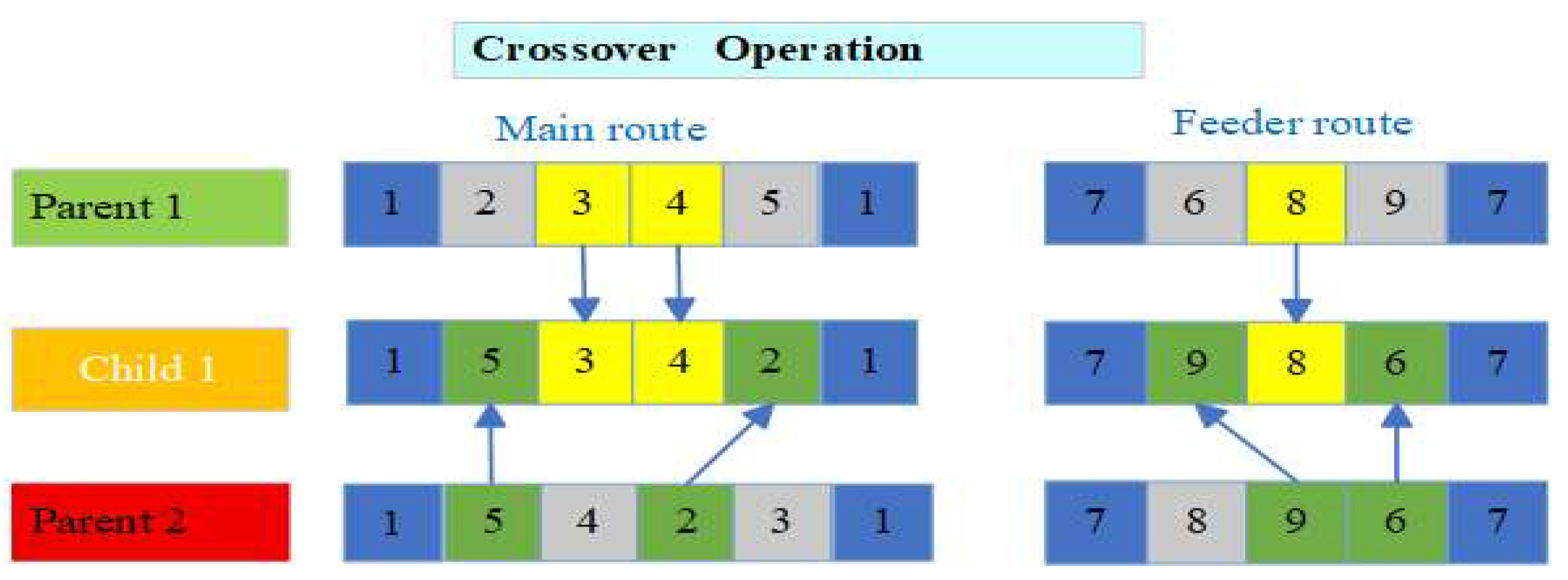
The crossover operation adopts the order crossover method to ensure that offspring do not visit the same port more than once. For the main route, if Parent 1 is [1, 2, 3, 4, 5, 1] and Parent 2 is [1, 5, 4, 2, 3, 1], a middle segment is selected: the segment [3, 4] from Parent 1 is fixed in the offspring at the same positions. Then, the remaining positions are filled in order from Parent 2, skipping the already included [3, 4]. The middle part of Parent 2 is [5, 4, 2, 3]; after removing [3, 4], the remaining [5, 2] are sequentially filled into the offspring, resulting in [1, 5, 3, 4, 2, 1].
For the feeder route, the chromosome encodes the path sequence from cargo source points to feeder ports. The crossover operation also uses the order crossover method, selecting a middle segment from one parent as a fixed part and filling the remaining feeder ports in order from the other parent while skipping duplicates. Since feeder routes have fewer nodes and are more localized, the order crossover effectively preserves local path continuity, improving scheduling efficiency and path rationality. Collect the cargo point assignments from both parent individuals, assign each cargo point to the nearest feeder port based on the shortest distance (nearest-first strategy), and construct the feeder route structure of the offspring chromosome. The detailed process is illustrated in Figure 5. In child 1, different colored squares are used, and each square comes from a square of the same color in the parent, indicated by arrows.
Figure 5.
Crossover operation.
Therefore, both the main and feeder routes use the order crossover method for crossover operations. However, the feeder route places more emphasis on local continuity and avoiding repeated visits, ensuring the overall path encoding is reasonable and effective.
Step 5: Mutation Operation.
We employ a swap mutation strategy to optimize the visiting sequence of ports. During mutation, only genes corresponding to the same route type (mainline or feeder route) are considered. Two intermediate ports are randomly selected and swapped within the offspring chromosome. This approach enhances population diversity and helps avoid premature convergence to local optima. By preserving the logical structure of each route while introducing variability, the GA maintains feasibility and improves exploration capability. The detailed mutation process is illustrated in Figure 6, and we transform child 1 into another child, which we call child *, and the color of the square is swapped, indicated by the arrow.
Figure 6.
Mutation operation.
Furthermore, we employ SA algorithm to solve the model as the second heuristic for comparisons. In brief, we introduce the logic of SA. First, an initial solution is generated. Second, new solutions are created through neighborhood exploration. Finally, the terminating solution is derived based on the SA acceptance function, cooling schedule, and termination criteria. The main steps are illustrated in Figure 5, and the SA solution flowchart is shown in Figure 6. Implementation Steps of the SA:
In each iteration, the scheduling cost of the current solution is first evaluated, and the cost difference between the newly generated solution and the current one is calculated. If the new solution has a lower cost, it is directly accepted as the current state. Otherwise, the inferior solution may still be accepted with a certain probability, which is determined by the following formula.
where T denotes the current temperature. As the temperature gradually decreases, SA’s tolerance for inferior solutions diminishes accordingly. Furthermore, to ensure that only feasible scheduling solutions are considered during the search process, each newly generated solution must undergo constraint validation. If any of the following basic constraints are violated, the solution is deemed infeasible and discarded:
- (1)
- The total vessel capacity must be sufficient to cover all loading and unloading demands along the route.
- (2)
- The arrival time at each port must comply with its designated service time window.
- (3)
- The total voyage time must not exceed the predefined maximum scheduling horizon.
The feasibility check can therefore be mathematically expressed as follows.
A scheduling solution is considered feasible only when it simultaneously satisfies all constraints, including vessel capacity limits, port service time windows, and the total voyage duration threshold. Otherwise, it is directly discarded and not subjected to the acceptance decision. Therefore, the final simulated annealing acceptance function is defined as follows.
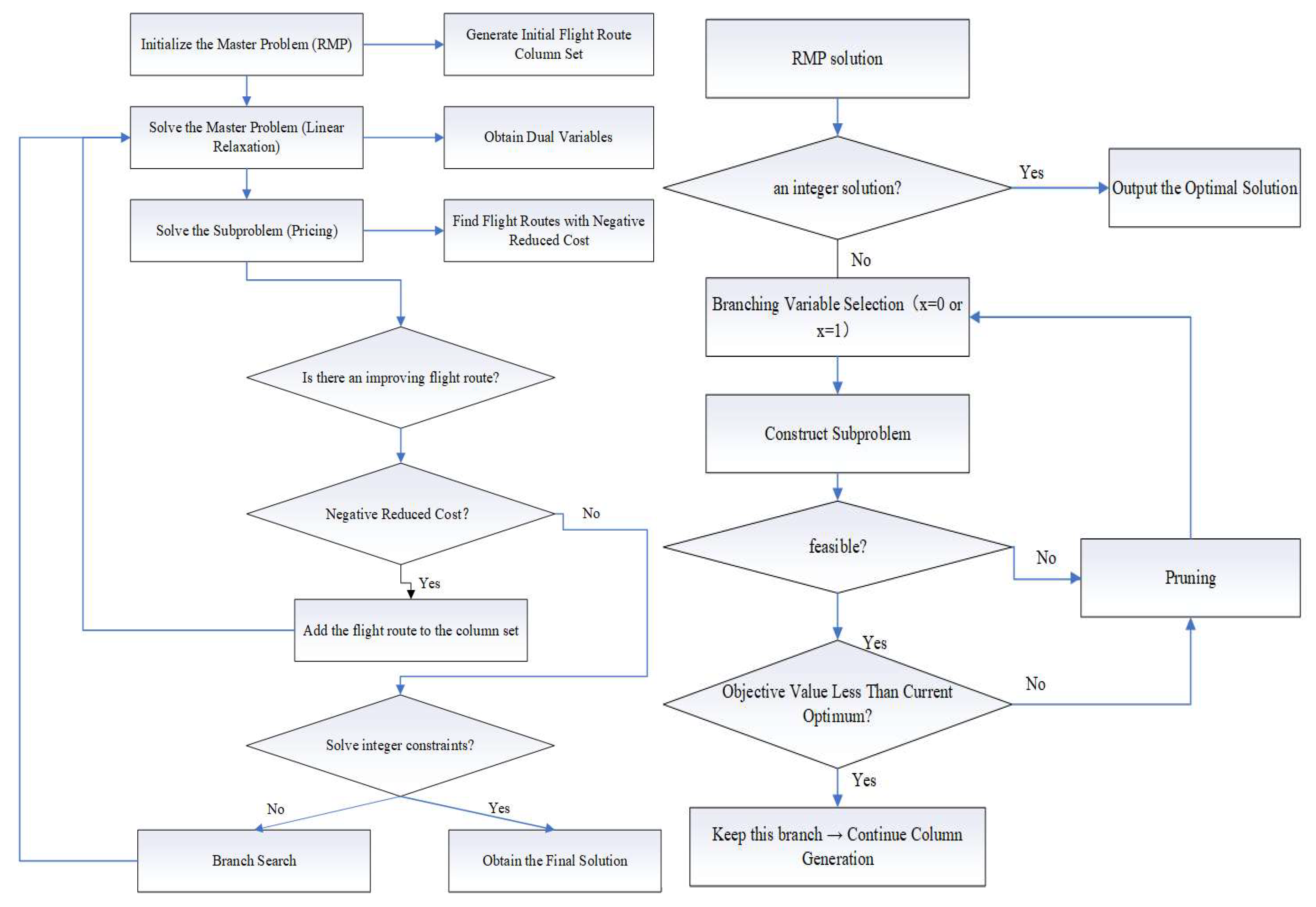
The following is the content of the B&P algorithm and its hybrid with GA and SA.
Step 1: First, formulate the RMP.
Based on a pre-generated fixed number of ports—such as one central hub port and several feeder ports—along with corresponding demand data, we first construct a set of initial feasible routing paths. These paths are treated as variable columns and imported into the RMP formulation.
To accelerate the convergence of the column generation process, we incorporate heuristic solutions as high-quality starting points for the B&P procedure. In particular, all integer decision variables are encoded in binary format, facilitating the branching process within the branch-and-bound framework.
Each route is represented as a “variable column” and includes the following structured information.
Port visiting sequence (route).
Total travel time.
Total transportation cost.
Feeder connection cost indicator.
Vessel type requirement.
The number of vessels required.
These routing variables are then used to construct the RMP in the following formula.
Solve the LP-relaxed RMP using Gurobi and record the dual values associated with all path variables.
Step 2: Column generation preprocessing.
In the B&P algorithm, column generation preprocessing is a critical step for initializing the master problem. This process ensures solvability of the initial RMP by generating a set of basic feasible routes for each feeder port with transportation demand. These initial routes are constructed in the form of “hub port → feeder port → hub port”, with cost and time estimated based on predefined vessel types. Each initial route is assigned a unique identifier, and a port-to-route coverage matrix is built to capture the inclusion relationships. To incorporate the feasibility of transshipment from source points to feeder ports, the preprocessing phase also enumerates and indexes all possible feeder paths between origin–destination port pairs. All such routes and related data are loaded into the master problem as the initial column set, providing a feasible solution.
Step 3: Pricing subproblem.
After each iteration of solving the RMP, new scheduling routes (variable columns) are constructed using the dual variables. If any of these routes have negative reduced cost, it indicates that the current solution of the master problem is not yet optimal. In such cases, the corresponding route is added to the RMP as a new variable column, and the process continues iteratively.
Step 3.1: Extract the dual variables (dual prices) from the RMP.
After solving the LP relaxation of the master problem, obtain the dual values (shadow prices) of each constraint from Gurobi.
Step 3.2: Enumerate the set of feasible candidate paths.
Construct a set of paths that start from the hub port and return to the hub port, satisfying the following constraints:
No repeated visits to the same port.
Feasibility with respect to vessel capacity and time window scheduling.
Control over the number of visited ports.
Step 3.3: Calculate the reduced cost of each path.
This step is one of the core components of the B&P, aiming to identify new routing paths with the potential to improve the current solution. It begins by extracting the dual variables associated with each constraint from the RMP. These dual values are then combined with the original transportation cost of each candidate path to calculate the reduced cost. Specifically, the reduced cost is obtained by subtracting the sum of the dual values corresponding to the ports involved in the path from its original cost. If the reduced cost of a path is negative, it indicates that the path can improve the current objective function and should be added as a new variable to the master problem for iterative solving. This mechanism dynamically generates valuable routes, effectively reducing the model size and accelerating convergence to the optimal solution, making it a key element for efficient column generation.
Step 3.4: Select the optimal paths and return them.
From the candidate paths, select the path(s) with the smallest (most negative) reduced cost. If there exists at least one path with a reduced cost less than zero, add it as a new column (variable) to the RMP. If no path with negative reduced cost exists, the current solution is the optimal solution of the RMP (under LP relaxation). Then return to Step 2 and continue iterating to solve the updated RMP.
Step 4: Branching strategy.
When the final solution of the RMP is non-integer, branching is required to divide the problem into several subproblems. These subproblems are then solved one by one to obtain an integer solution. The branching operation is shown in Figure 6.
Step 5: Node processing.
Case 1: If the solution at the current node is integer, it represents a feasible integer scheduling solution. Calculate its total cost (objective value) and compare it with the current Best Integer Solution: if it is better → update the best solution; otherwise → discard it.
Case 2: If the solution is non-integer, further branching is required (proceed to Step 4).
Case 3: If the lower bound of the LP solution at the current node exceeds the current best integer solution, it indicates no better solution can be found from this node → prune it.
Case 4: If the current node violates constraints (no feasible path), it is deemed infeasible → prune it.
The final output includes the following: (i) the optimal route combination, covering both mainline and feeder scheduling routes; (ii) the total cost, consisting of mainline transport, feeder connections, and port handling charges; (iii) the total time consumption, including sailing time, feeder transfer time, and loading/unloading durations; (iv) the visit status and service path for each port, indicating whether it is served by mainline or feeder vessels; the vessel configuration and resource allocation plan, detailing the type, number, and deployment of vessels across all routes, the feeder design, outlining connection plans from cargo source points to feeder ports, verifying all constraints (capacity, time window, feasibility), and specifying feeder routes, related costs, and transit times. This comprehensive output ensures efficient coordination between mainline and feeder transport within the scheduling framework.
5. Case Study
To validate the applicability and scalability of the proposed prediction–optimization integrated scheduling approach, this study conducts experimental analyses on three representative cases: (a) a small-scale Japan–Korea near-sea network (15–24 ports); (b) a medium-scale Southeast Asia–China regional hub network (24–33 ports), and (c) a large-scale Asia–Europe Ocean network (more than 33 ports). In Table 3, the interval numbers in each port type for the three case categories are presented, and in Table 4, the parameters in each vessel type are shown. The following presents the route diagram for the small-scale case in Figure 7. The base map of Figure 7 is sourced from Google Maps, available at: http://www.gditu.net/ (accessed on 2025. 05. 11) , and the black arrows connect the main routing, and orange arrows connect the feeder routing. To support model solution and validation, this study rigorously constructed a reproducible computing environment to ensure the rigor of the experimental results and their applicability to small, medium, and large-scale scenarios. Regarding hardware, the computer performance is as follows: an Intel Core i7-8750H processor (base frequency 3.6 GHz, maximum turbo frequency 5.0 GHz) provides powerful parallel computing capabilities; 32 GB of DDR4 memory (3200 MHz) fully meets the memory requirements of mixed-integer linear programming (MILP) models in high-dimensional networks; and the operating system is Windows 10 Professional (64-bit), ensuring stability during the development and solution process. Regarding software, Python 3.8.12 is used as the core development environment, and Gurobi 9.5.0 is integrated as the MILP solver, supporting efficient solution of the main problem and subproblems in the branch-and-price (B&P) algorithm. TensorFlow 2.7.0 is used to train a long short-term memory network (LSTM) demand forecasting model, providing accurate input for optimization.
Table 3.
Number ranges of ports for the three types of cases.
Table 4.
Information on different types of vessels.
Figure 7.
Small-scale case illustration (Japan–Korea).
5.1. Data Input
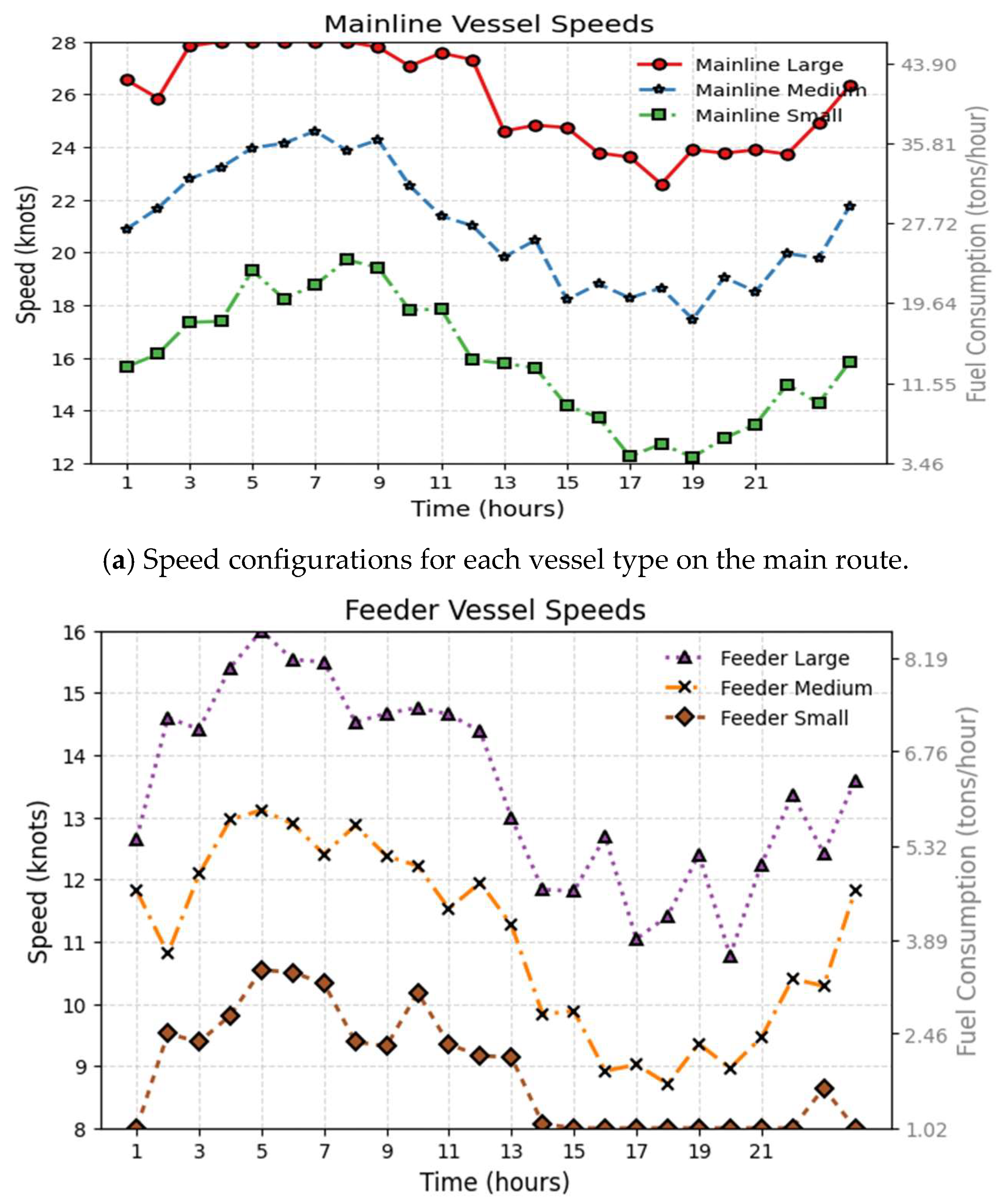
For each vessel type’s speed configuration, including large, medium, and small vessels on the main route as well as large, medium, and small vessels on the feeder segment, the results obtained as per different algorithms are presented in Figure 8.
Figure 8.
Speed configurations for each vessel type.
5.2. Computational Results
The optimized solutions for the three types of cases differ under the heuristic and exact algorithms. When the number of visited ports on the main route ranges between 5 and 20, the corresponding optimal paths are shown in Table A1. In Table A1, the optimal visiting sequences of the main routes obtained by each algorithm are presented for different numbers of ports to be visited (ranging from 5 to 20). For example, the sequence (13541) indicates that, when the total number of visited ports is 5, the optimal route under the heuristic algorithm is: Port 1, Port 3, Port 5, Port 4, Port 1. In Table A2, “1” denotes the hub port. In addition, the optimal results for the feeder routes are shown in Table A1. For the small, medium, and large case types, different optimal solutions are obtained using five different algorithms. In addition, the optimal results for the feeder routes are shown in Table A2.
For the small, medium, and large case types, different optimal solutions (in million USD) are obtained using five different algorithms. The detailed results are presented in Table A3, Table A4, and Table A5, respectively.
Moreover, when the number of port intervals in each case ranges from 5 to 20, the runtime comparison between the heuristic and heuristic + exact algorithms is shown in Table A6.
The optimized solution obtained by the multiple algorithms and the specific result data of each algorithm are reflected in the Appendix A (Table A1, Table A2, Table A3, Table A4, Table A5 and Table A6).
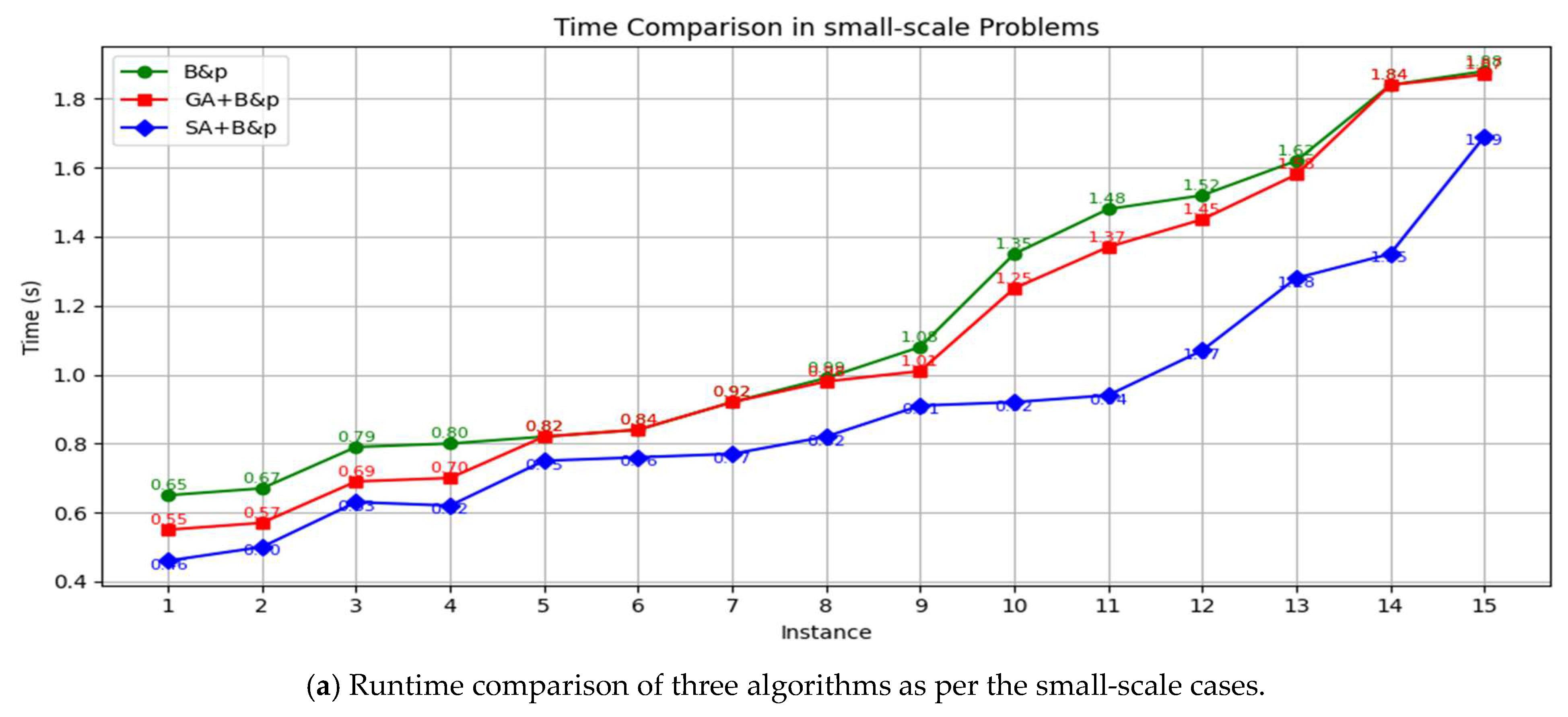
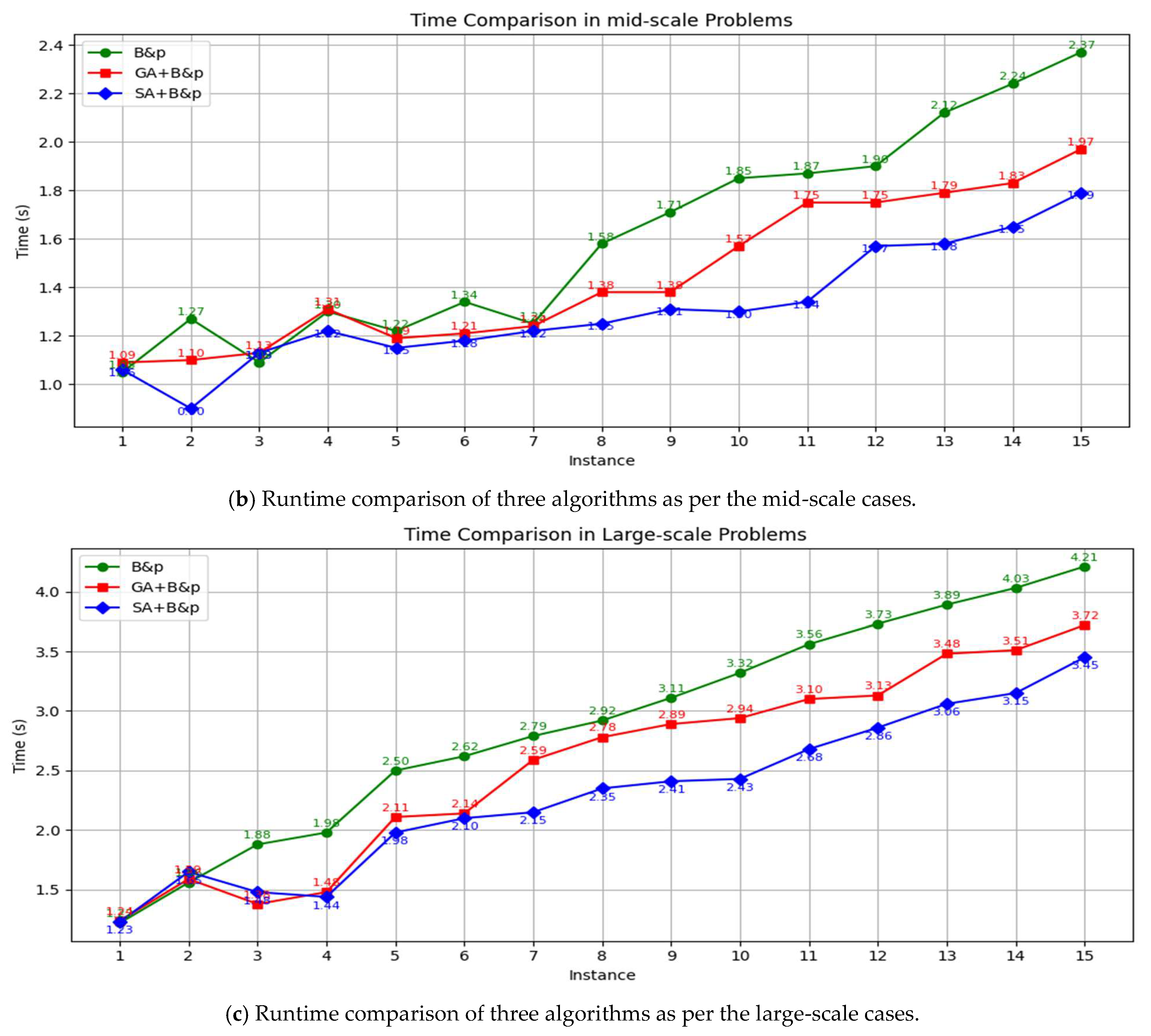
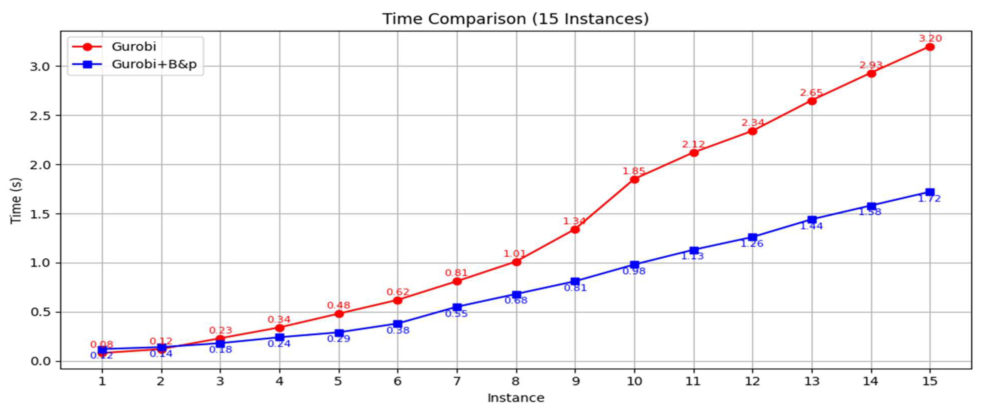
According to the experimental results across small, medium, and large-scale port combinations, the hybrid strategies that integrate GA or SA with the B&P algorithm consistently outperform traditional standalone algorithms. In particular, the SA + B&P method achieves the lowest total cost in most test cases, demonstrating superior stability and solution quality. As the number of visited ports and network complexity increase, the overall improvement rate becomes more significant—rising from approximately 0.19% to 1.9% in small-scale cases, 0.94% to 4.51% in medium-scale cases, and even exceeding 8% in large-scale scenarios—indicating that the hybrid approach is especially effective for complex route planning problems. While the standalone B&P algorithm performs well in some small instances, it tends to show fluctuations in efficiency and solution quality in larger cases. Overall, the proposed hybrid optimization approach not only improves the optimality of the objective function but also demonstrates strong scalability, making it suitable for real-world multi-port container liner scheduling optimization. In each case, 15 representative port combinations were selected to compare the runtime performance of hybrid heuristic (SA/GA) + exact algorithm (B&P) with that of the standalone exact algorithm (B&P), as well as with a commercial solver (Groubi), The specific comparisons are shown in Figure 9, Moreover, the BP algorithm is integrated into the commercial solver to obtain the optimized runtime comparison chart in Figure 10.

Figure 9.
Comparison of running times across three cases.
Figure 10.
Comparison between B&P with Gurobi.
The results on small, medium, and large-scale multi-port combinations show that compared with the traditional GA, the SA + B&P hybrid algorithm reduces the total transportation cost by approximately 0.81% to 8.08% on average, with a maximum optimization improvement of 8.08%, while cutting computation time by about 16.86% to 24.7%, demonstrating superior algorithmic stability and scalability. The incorporation of dynamic demand forecasting significantly enhances the adaptability and accuracy of scheduling plans, effectively mitigating uncertainties caused by fluctuations in loading volumes. The dynamic feeder allocation mechanism rationally distributes feeder transport resources, optimizes mainline load, and improves overall transportation efficiency. The multi-objective scheduling framework achieves a balanced trade-off between economic and time costs, meeting the diverse demands of practical operations. In summary, the integrated optimization proposed in this study improves both the cost-effectiveness and computational efficiency of multi-port liner scheduling. By incorporating dynamic demand forecasting, a three-level transportation network, and hybrid optimization methods, the study provides accurate, adaptive, and efficient scheduling solutions. The results demonstrate its practical value in reducing costs, saving running time, and enhancing overall transportation efficiency, offering solid support for the development of intelligent and digitalized liner shipping systems.
6. Conclusions
This study addresses the multi-port routing and scheduling issues in modern container liner shipping. We propose a comprehensive optimization framework that integrates dynamic demand forecasting, a three-level transportation network, and hybrid optimization strategies. Specifically, this framework unifies demand forecasting, network modeling, and algorithmic optimization to holistically characterize the interactions among demand fluctuations, hub-feeder coordination, and vessel scheduling decisions. The study establishes a hierarchical structure composed of hub ports, feeder ports, and cargo sources to achieve effective integration of trunk and feeder line transportation.
The three real cases evaluate the prediction accuracy, scheduling model’s effectiveness, and algorithm solution efficiency under different network scales. In all the cases, the port system is categorized into hub ports, feeder ports, and origin points, reflecting a real “trunk-feeder combined” transportation structure. In the medium- and large-scale cases, this hierarchical network structure is more pronounced, requiring coordinated scheduling between mainline and feeder routes. This setup highlights the advantages of integrated scheduling involving multiple ports, vessels, and transport segments, effectively overcoming the modeling limitations of traditional VRP or single-vessel approaches. Moreover, in all cases, port loading and unloading demands are predicted using deep learning techniques (i.e., LSTM), enabling more timely and accurate cargo flow information prior to optimization. This predictive mechanism improves voyage scheduling rationality and turnaround efficiency in the small-scale case. In medium- and large-scale networks, it becomes a crucial tool for achieving capacity matching and dynamic route adjustments during scheduling, thereby reducing empty sailing risks and minimizing resource waste. To further enhance the quality of scheduling solutions and the adaptability of the algorithm, this study evaluates the optimization performance of standalone heuristic algorithms (GA, SA) and hybrid strategies combining heuristics with exact algorithms (GA + B&P, SA + B&P) across the three cases. Among these, SA + B&P performs best in terms of cost reduction and computational efficiency.
In our future research plans, we will primarily focus on advancing the development of ship propulsion sources, expanding propulsion systems from traditional fuel-powered systems to hybrid power systems combining fuel and electricity. Simultaneously, we will integrate stochastic optimization and robust optimization methods to address uncertainties arising from demand forecasting errors, fluctuations in port turnaround times, and variations in navigation power supply under different sea states. Given that existing models typically assume port cooperation, while reality often involves competition between ports, we will address this limitation by incorporating competitive dynamics into our analysis. Furthermore, to enhance the practical applicability of machine learning-based demand forecasting, the research will further explore its robustness, ensuring the reliability of forecast results under various operating environments.
Author Contributions
Conceptualization, Z.C., T.Q., S.Z., H.S. and Y.T.; methodology, Z.C., T.Q., S.Z., H.S. and Y.T.; software, Z.C., T.Q., S.Z., H.S. and Y.T.; validation, Z.C., T.Q., S.Z., H.S. and Y.T.; formal analysis, Z.C., T.Q., S.Z., H.S. and Y.T.; investigation, Z.C., T.Q., S.Z., H.S. and Y.T.; resources, Z.C., T.Q., S.Z., H.S. and Y.T.; data curation, Z.C., T.Q., S.Z., H.S. and Y.T.; writing—original draft preparation, Z.C., T.Q., S.Z., H.S. and Y.T.; writing—review and editing, Z.C., T.Q., S.Z., H.S. and Y.T.; visualization, Z.C., T.Q., S.Z., H.S. and Y.T.; supervision, Z.C. and S.Z.; project administration, Z.C. and S.Z.; funding acquisition, Z.C. and S.Z. All authors have read and agreed to the published version of the manuscript.
Funding
This study is supported by the Nantong University Base of the Jiangsu Research Center for Xi Jinping Thought on Socialism with Chinese Characteristics for a New Era (25jdyb010), by the 2025 Jiangsu Provincial Science and Technology Think Tank Youth Initiative Program (JSKX 0125 086), by the Jiangsu Provincial Social Science Foundation Project (25ZHB022), and by the Engineering Research Center of Sustainable Urban Intelligent Transportation, Ministry of Education Open Project Funding (KCX2024-KF02).
Data Availability Statement
Data are contained within the article.
Conflicts of Interest
Author Haibo Song was employed by the company CRRC Intelligent Transportation Engineering Technology Co., Ltd. The remaining authors declare that the research was conducted in the absence of any commercial or financial relationships that could be construed as a potential conflict of interest.
Appendix A
The appendix presents detailed results of multi-port liner vessel routing and scheduling optimization experiments through Table A1, Table A2, Table A3, Table A4, Table A5 and Table A6. Table A1 lists the optimal main route sequences generated by various algorithms under different numbers of port visits (from 5 to 20 ports), and the “1*”represents hub port, which may be the same as the initial hub port or a different hub port. Table A2 provides the optimal routes for feeder transportation. Table A3, Table A4 and Table A5 compare the total costs (in thousand USD) of the algorithms in small, medium, and large-scale cases, indicating that dynamic demand forecasting and hybrid strategies can significantly reduce costs (with a maximum improvement of 8.08%). Finally, Table A6 compares the running times of the algorithms, demonstrating that the hybrid method improves computational efficiency while maintaining quality (saving up to 24.7% of time).
Table A1.
Optimal main routes for port visits in the range of 5 to 20.
Table A1.
Optimal main routes for port visits in the range of 5 to 20.
| Optimal Route (Ports Visited) | Small-Scale | Medium-Scale | Large-Scale | |||
|---|---|---|---|---|---|---|
| GA/SA | B&P + GA/SA | GA/SA | B&P + GA/SA | GA/SA | B&P + GA/SA | |
| 5 | (1, 3, 5, 4, 1) | (1, 3, 6, 4, 1) | (1, 2, 4, 3, 1) | (1, 2, 3, 4, 1) | (1, 6, 7, 5, 1 *) | (1, 2, 3, 4, 1 *) |
| 6 | (1, 2, 3, 5, 4, 1) | (1, 3, 2, 5, 6, 1) | (1, 4, 3, 5, 7, 1) | (1, 4, 6, 5, 7, 1) | (1, 3, 4, 5, 7, 1) | (1, 2, 4, 5, 7, 1 *) |
| 7 | (1, 2, 3, 5, 6, 4, 1) | (1, 3, 2, 5, 6, 4, 1) | (1, 7, 3, 5, 2, 4, 1) | (1, 6, 3, 5, 2, 4, 1) | (1, 2, 3, 5, 7, 6, 1*) | (1, 3, 2, 5, 7, 6, 1 *) |
| 8 | (1, 4, 3, 5, 7, 6, 2, 1) | (1, 3, 4, 5, 7, 6, 2, 1) | (1, 4, 7, 8, 6, 2, 3, 1) | (1, 2, 4, 8, 7, 5, 3, 1) | (1, 2, 3, 5, 8, 7, 6, 1 *) | (1, 5, 2, 3, 7, 6, 4, 1 *) |
| 9 | (1, 3, 4, 8, 7, 5, 6, 2, 1) | (1, 4, 3, 5, 8, 7, 2, 6, 1) | (1, 4, 7, 8, 9, 6, 2, 3, 1) | (1, 2, 4, 8, 9, 7, 5, 3, 1) | (1, 3, 4, 5, 9, 8, 7, 6, 1 *) | (1, 4, 3, 5, 7, 6, 4, 2, 1 *) |
| 10 | (1, 2, 3, 5, 6, 7, 4, 8, 9, 1) | (1, 3, 2, 5, 6, 7, 4, 8, 10, 1) | (1, 4, 5, 7, 8, 6, 2, 3, 9, 1) | (1, 4, 5, 6, 7, 9, 8, 3, 2, 1) | (1, 2, 4, 5, 6, 8, 9, 10, 7, 1 *) | (1, 5, 2, 3, 6, 8, 9, 10, 4, 1 *) |
| 11 | (1, 2, 3, 5, 6, 7, 4, 8, 9, 10, 1) | (1, 3, 2, 5, 6, 7, 4, 8, 10, 11, 1) | (1, 4, 5, 7, 8, 6, 2, 3, 9, 10, 1) | (1, 4, 5, 6, 7, 9, 8, 3, 2, 10, 1) | (1, 2, 4, 5, 6, 8, 9, 10, 7, 11, 1 *) | (1, 5, 2, 3, 6, 8, 9, 10, 4, 11, 1 *) |
| 12 | (1, 2, 3, 5, 6, 7, 4, 8, 9, 10, 11, 1) | (1, 3, 2, 5, 6, 7, 4, 8, 10, 11, 12, 1) | (1, 4, 5, 7, 8, 6, 2, 3, 9, 10, 11, 1) | (1, 4, 5, 6, 7, 9, 8, 3, 2, 10, 11, 1) | (1, 2, 4, 5, 6, 8, 9, 10, 7, 11, 12, 1 *) | (1, 5, 2, 3, 6, 8, 9, 10, 4, 11, 12, 1 *) |
| 13 | (1, 2, 3, 5, 6, 7, 4, 8, 9, 10, 11, 12, 1) | (1, 3, 2, 5, 6, 7, 4, 8, 10, 11, 12, 13, 1) | (1, 4, 5, 7, 8, 6, 2, 3, 9, 10, 11, 12, 1) | (1, 4, 5, 6, 7, 9, 8, 3, 2, 10, 11, 12, 1) | (1, 2, 4, 5, 6, 8, 9, 10, 7, 11, 12, 13, 1 *) | (1, 5, 2, 3, 6, 8, 9, 10, 4, 11, 12, 13, 1 *) |
| 14 | (1, 2, 3, 5, 6, 7, 4, 8, 9, 10, 11, 12, 13, 1) | (1, 3, 2, 5, 6, 7, 4, 8, 10, 11, 12, 13, 14, 1) | (1, 4, 5, 7, 8, 6, 2, 3, 9, 10, 11, 12, 13, 1) | (1, 4, 5, 6, 7, 9, 8, 3, 2, 10, 11, 12, 13, 1) | (1, 2, 4, 5, 6, 8, 9, 10, 7, 11, 12, 13, 14, 1 *) | (1, 5, 2, 3, 6, 8, 9, 10, 4, 11, 12, 13, 14, 1 *) |
| 15 | (1, 2, 3, 5, 6, 7, 4, 8, 9, 10, 11, 12, 13, 14, 1) | (1, 3, 2, 5, 6, 7, 4, 8, 10, 11, 12, 13, 14, 9, 1) | (1, 4, 5, 7, 8, 6, 2, 3, 9, 10, 11, 12, 13, 14, 1) | (1, 4, 5, 6, 7, 9, 8, 3, 2, 10, 11, 12, 13, 14, 1) | (1, 2, 4, 5, 6, 8, 9, 10, 7, 11, 12, 13, 14, 15, 1 *) | (1, 5, 2, 3, 6, 8, 9, 10, 4, 11, 12, 13, 14, 15, 1 *) |
| 16 | (1, 2, 3, 5, 6, 7, 4, 8, 9, 10, 11, 12, 13, 14, 15, 1) | (1, 3, 2, 5, 6, 7, 4, 8, 10, 11, 12, 13, 14, 15, 16, 1) | (1, 4, 5, 7, 8, 6, 2, 3, 9, 10, 11, 12, 13, 14, 15, 1) | (1, 4, 5, 6, 7, 9, 8, 3, 2, 10, 11, 12, 13, 14, 16, 1) | (1, 2, 4, 5, 6, 8, 9, 10, 7, 11, 12, 13, 14, 15, 16, 1 *) | (1, 5, 2, 3, 6, 8, 9, 10, 4, 11, 12, 13, 14, 15, 16, 1 *) |
| 17 | (1, 2, 3, 5, 6, 7, 4, 8, 9, 10, 11, 12, 13, 14, 15, 16, 1) | (1, 3, 2, 5, 6, 7, 4, 8, 10, 11, 12, 13, 14, 15, 16, 17, 1) | (1, 4, 5, 7, 8, 6, 2, 3, 9, 10, 11, 12, 13, 14, 15, 16, 1) | (1, 4, 5, 6, 7, 9, 8, 3, 2, 10, 11, 12, 13, 14, 16, 17, 1) | (1, 2, 4, 5, 6, 8, 9, 10, 7, 11, 12, 13, 14, 15, 16, 17, 1 *) | (1, 5, 2, 3, 6, 8, 9, 10, 4, 11, 12, 13, 14, 15, 16, 17, 1 *) |
| 18 | (1, 2, 3, 5, 6, 7, 4, 8, 9, 10, 11, 12, 13, 14, 15, 16, 17, 1) | (1, 3, 2, 5, 6, 7, 4, 8, 10, 11, 12, 13, 14, 15, 16, 17, 18, 1) | (1, 4, 5, 7, 8, 6, 2, 3, 9, 10, 12, 11, 13, 14, 15, 16, 17, 1) | (1, 4, 5, 6, 7, 9, 8, 3, 2, 10, 11, 12, 13, 14, 16, 17, 18, 1) | (1, 2, 4, 5, 6, 8, 9, 10, 7, 11, 12, 13, 14, 15, 16, 17, 18, 1 *) | (1, 5, 2, 3, 6, 8, 9, 10, 4, 11, 12, 13, 14, 15, 16, 17, 18, 1 *) |
| 19 | (1, 2, 3, 5, 6, 7, 4, 8, 9, 10, 11, 12, 13, 14, 15, 16, 17, 18, 1) | (1, 3, 2, 5, 6, 7, 4, 8, 10, 11, 12, 13, 14, 15, 16, 17, 18, 19, 1) | (1, 4, 5, 7, 8, 6, 2, 3, 9, 10, 11, 12, 13, 14, 15, 16, 17, 18, 1) | (1, 4, 5, 6, 7, 9, 8, 3, 2, 10, 11, 12, 13, 14, 16, 17, 18, 19, 1) | (1, 2, 4, 5, 6, 8, 9, 10, 7, 11, 12, 13, 14, 15, 16, 17, 18, 19, 1 *) | (1, 5, 2, 3, 6, 8, 9, 10, 4, 11, 12, 13, 14, 15, 16, 17, 18, 19, 1 *) |
| 20 | (1, 2, 3, 5, 6, 7, 4, 8, 9, 10, 11, 12, 13, 14, 15, 16, 17, 18, 19, 1) | (1, 3, 2, 5, 6, 7, 4, 8, 10, 11, 12, 13, 14, 15, 16, 17, 18, 19, 20, 1) | (1, 4, 5, 7, 8, 6, 2, 3, 9, 10, 11, 12, 13, 14, 15, 16, 17, 18, 19, 1) | (1, 4, 5, 6, 7, 9, 8, 3, 2, 10, 11, 12, 13, 14, 16, 17, 18, 19, 20, 1) | (1, 2, 4, 5, 6, 8, 9, 10, 7, 11, 12, 13, 14, 15, 16, 18, 17, 19, 20, 1 *) | (1, 5, 2, 3, 6, 8, 9, 10, 4, 11, 12, 13, 14, 15, 16, 17, 18, 19, 20, 1 *) |
Table A2.
Optimal feeder routes for port visits in the range of 5 to 20.
Table A2.
Optimal feeder routes for port visits in the range of 5 to 20.
| Optimal Route (Ports Visited) | Small-Scale | Medium-Scale | Large-Scale | |||
|---|---|---|---|---|---|---|
| GA/SA | B&P + GA/SA | GA/SA | B&P + GA/SA | GA/SA | B&P + GA/SA | |
| 5 | (2, 1) | (2, 1), (5, 4) | (1, 5, 6, 7, 1) | (1, 5, 6, 7, 1) | (2, 1), (3, 5), (4, 5) | (1, 5, 6, 7, 1) |
| 6 | (6, 7, 8, 9, 6) | (4, 3) | (2, 1), (6, 5) | (2, 1), (3, 4) | (2, 1), (6, 5) | (3, 4), (6, 5) |
| 7 | (7, 8, 9, 10, 7) | (7, 10, 11, 12, 7) | (5, 6, 7, 8, 5) | (5, 8, 7, 6, 5) | (7, 8, 9, 10, 7) | (7, 9, 8, 10, 7) |
| 8 | (8, 7, 9, 10, 8) | (9, 10, 1) | (9, 10, 11, 12, 9) | (9, 11, 10, 12, 9) | (8, 9, 10, 11, 8) | (8, 9, 11, 10, 8) |
| 9 | (9, 8, 10, 9) | (9, 7, 11, 9) | (10, 11, 12, 13, 10) | (10, 13, 12, 11, 10) | (10, 11, 12, 13, 10) | (10, 1213, 11, 10) |
| 10 | (10, 9) | (9, 8) | (11, 12, 13, 14, 11) | (11, 14, 13, 12, 11) | (11, 12, 13, 14, 11) | (11, 13, 12, 14, 11) |
| 11 | (11, 10) | (12, 8) | (12, 14, 13, 15, 12) | (12, 15, 13, 14, 12) | (12, 13, 14, 15, 12) | (12, 15, 14, 13, 12) |
| 12 | (12, 11) | (13, 8) | (13, 14, 15, 16, 13) | (13, 14, 16, 15, 13) | (13, 14, 15, 16, 13) | (13, 15, 16, 14, 13) |
| 13 | (13, 12) | (14, 8) | (14, 15, 16, 17, 14) | (14, 17, 15, 16, 14) | (14, 15, 16, 17, 14) | (14, 15, 17, 16, 14) |
| 14 | (14, 13) | (15, 8) | (15, 16, 17, 18, 15) | (15, 18, 16, 17, 15) | (15, 16, 17, 18, 15) | (15, 18, 16, 17, 15) |
| 15 | (15, 14) | (9, 14) | (16, 17, 18, 19, 16) | (16, 18, 19, 17, 16) | (16, 17, 18, 19, 16) | (16, 17, 19, 18, 16) |
| 16 | (16, 15) | (17, 16) | (17, 18, 19, 20, 17) | (17, 21, 19, 20, 17) | (17, 18, 19, 20, 17) | (17, 20, 18, 19, 17) |
| 17 | (17, 16) | (18, 17) | (18, 17, 20, 21, 18) | (18, 20, 21, 19, 18) | (18, 19, 20, 21, 18) | (18, 21, 20, 19, 18) |
| 18 | (18, 17) | (19, 18) | (19, 20, 21, 22, 19) | (19, 21, 22, 20, 19) | (19, 20, 21, 22, 19) | (19, 21, 22, 20, 19) |
| 19 | (19, 18) | (20, 19) | (18, 19, 20, 22, 21, 18) | (18, 20, 22, 21, 18) | (19, 21, 22, 24, 20, 19) | (19, 20, 22, 24, 21, 19) |
| 20 | (20, 21, 22, 23, 20) | (21, 22, 24, 21) | (17, 20, 21, 22, 17) | (17, 21, 22, 20, 17) | (20, 21, 23, 24, 20) | (20, 23, 21, 20) |
Table A3.
Objective value(/$1000) comparison under small-scale case with selected port visit numbers.
Table A3.
Objective value(/$1000) comparison under small-scale case with selected port visit numbers.
| Combination | Optimal Route (Ports Visited) | GA | SA | BP | GA + BP | SA + BP | Improvement Rate |
|---|---|---|---|---|---|---|---|
| (1, 7, 14) | 5 | 1853.4 | 1840.4 | 1833.3 | 1833.3 | 1826.7 | 1.44% |
| (1, 5, 10) | 5 | 1820.1 | 1806.7 | 1806.5 | 1805.4 | 1795.8 | 1.33% |
| (1, 6, 10) | 5 | 1857.6 | 1842.8 | 1840.2 | 1835.9 | 1843.5 | 1.17% |
| (1, 7, 11) | 6 | 1832.5 | 1821.5 | 1820.6 | 1819.4 | 1830.5 | 0.72% |
| (1, 7, 12) | 6 | 1845.4 | 1838.9 | 1839.9 | 1832.5 | 1830.8 | 0.79% |
| (1, 7, 10) | 6 | 1854.8 | 1853.7 | 1854.8 | 1833.7 | 1832.8 | 1.19% |
| (1, 8, 15) | 7 | 1857.8 | 1855.6 | 1857.3 | 1854.8 | 1832.9 | 1.3% |
| (1, 8, 14) | 7 | 1858.4 | 1856.8 | 1857.2 | 1855.4 | 1834.8 | 1.2% |
| (1, 8, 13) | 7 | 1868.4 | 1867.3 | 1866.5 | 1856.4 | 1836.3 | 1.7% |
| (1, 8, 12) | 8 | 1869.5 | 1866.8 | 1867.9 | 1865.7 | 1843.3 | 1.4% |
| (1, 8, 11) | 8 | 1870.8 | 1869.8 | 1870.1 | 1868.7 | 1833.8 | 1.9% |
| (1, 7, 15) | 8 | 1871.8 | 1868.7 | 1869.0 | 1868.4 | 1868.3 | 0.19% |
| (1, 7, 13) | 5 | 1872.8 | 1870.8 | 1871.8 | 1868.6 | 1867.3 | 0.29% |
| (1, 7, 9) | 5 | 1876.3 | 1874.5 | 1875.4 | 1873.5 | 1872.5 | 0.20% |
| (1, 7, 8) | 5 | 1875.8 | 1873.2 | 1873.5 | 1872.5 | 1871.5 | 0.23% |
Table A4.
Objective values(/$1000)—medium case selected port visits.
Table A4.
Objective values(/$1000)—medium case selected port visits.
| Combination | Optimal Route (Ports Visited) | GA | SA | BP | GA + BP | SA + BP | Improvement Rate |
|---|---|---|---|---|---|---|---|
| (1, 8, 15) | 6 | 2645.8 | 2648.7 | 2644.3 | 2630.5 | 2622.8 | 0.98% |
| (1, 8, 16) | 6 | 2655.7 | 2638.7 | 2621.8 | 2610.7 | 2589.6 | 2.49% |
| (1, 8, 17) | 6 | 2674.6 | 2666.8 | 2650.7 | 2643.8 | 2635.7 | 1.46% |
| (1, 8, 18) | 7 | 2688.7 | 2666.1 | 2653.7 | 2629.7 | 2611.8 | 2.86% |
| (1, 8, 19) | 7 | 2688.8 | 2666.3 | 2654.2 | 2621.5 | 2610.4 | 2.92% |
| (1, 9, 18) | 7 | 2699.2 | 2688.4 | 2665.7 | 2631.7 | 2610.8 | 3.28% |
| (1, 9, 19) | 8 | 2700.5 | 2699.3 | 2693.5 | 2681.2 | 2635.4 | 2.41% |
| (1, 10, 15) | 8 | 2740.8 | 2733.5 | 2730.7 | 2701.8 | 2689.6 | 1.87% |
| (1, 10, 16) | 8 | 2755.1 | 2744.6 | 2714.6 | 2700.8 | 2697.3 | 2.10% |
| (1, 12, 20) | 9 | 2786.3 | 2755.3 | 2740.1 | 2714.8 | 2700.5 | 3.08% |
| (1, 12, 18) | 9 | 2760.5 | 2739.8 | 2710.1 | 2700.7 | 2667.8 | 3.36% |
| (1, 12, 19) | 9 | 2755.8 | 2732.7 | 2690.0 | 2677.4 | 2660.3 | 3.47% |
| (1, 12, 15) | 10 | 2733.8 | 2730.8 | 2721.8 | 2688.6 | 2667.3 | 2.43% |
| (1, 12, 16) | 10 | 2746.3 | 2734.5 | 2643.4 | 2633.5 | 2622.5 | 4.51% |
| (1, 10, 18) | 10 | 2700.8 | 2698.2 | 2688.5 | 2681.5 | 2675.5 | 0.94% |
Table A5.
Objective value(/$1000) comparison under large-scale case with selected port visit numbers.
Table A5.
Objective value(/$1000) comparison under large-scale case with selected port visit numbers.
| Combination | Optimal Route (Ports Visited) | GA | SA | BP | GA + BP | SA + BP | Improvement Rate |
|---|---|---|---|---|---|---|---|
| (2, 10, 20) | 8 | 2069.5 | 2066.8 | 2067.9 | 2065.7 | 2043.3 | 1.27% |
| (2, 11, 21) | 8 | 2170.8 | 2169.5 | 2170.2 | 2168.8 | 2133.1 | 1.73% |
| (2, 12, 22) | 8 | 2271.8 | 2268.7 | 2369.0 | 2368.4 | 2368.3 | 4.23% |
| (2, 13, 23) | 9 | 2457.4 | 2455.0 | 2457.5 | 2453.1 | 2432.9 | 1.00% |
| (2, 14, 24) | 9 | 2558.8 | 2556.8 | 2557.2 | 2555.4 | 2534.4 | 0.95% |
| (2, 15, 25) | 9 | 2668.4 | 2667.2 | 2666.4 | 2646.7 | 2656.8 | 0.81% |
| (2, 15, 24) | 10 | 2769.5 | 2766.8 | 2767.9 | 2735.7 | 2713.3 | 2.02% |
| (2, 15, 23) | 10 | 2872.8 | 2879.8 | 2871.1 | 2818.7 | 2813.8 | 2.29% |
| (2, 15, 22) | 10 | 2958.4 | 2956.8 | 2957.2 | 2955.4 | 2924.8 | 1.13% |
| (2, 15, 21) | 11 | 3068.4 | 3067.3 | 3066.5 | 3016.4 | 3026.3 | 1.70% |
| (2, 14, 20) | 11 | 3169.5 | 3166.8 | 3167.9 | 3165.7 | 3033.3 | 4.30% |
| (2, 13, 24) | 11 | 3270.8 | 3269.8 | 3270.1 | 3268.5 | 3013.4 | 7.87% |
| (2, 13, 22) | 12 | 3371.3 | 3368.8 | 3369.4 | 3308.2 | 3098.8 | 8.08% |
| (2, 13, 21) | 12 | 3472.8 | 3470.8 | 3471.8 | 3458.8 | 3267.3 | 5.91% |
| (2, 12, 20) | 12 | 3476.3 | 3474.5 | 3475.4 | 3373.5 | 3272.5 | 5.87% |
Table A6.
Running times (/s) of executing different algorithms.
Table A6.
Running times (/s) of executing different algorithms.
| Optimal Route (Ports Visited) | Small-Scale | Medium-Scale | Large-Scale | |||
|---|---|---|---|---|---|---|
| B&P | B&P + GA/SA | B&P | B&P + GA/SA | B&P | B&P + GA/SA | |
| 5 | 1.55 | 1.32/1.20 | 1.56 | 1.22/1.20 | 1.50 | 1.22/1.20 |
| 6 | 1.68 | 1.56/1.52 | 1.78 | 1.56/1.32 | 1.88 | 1.56/1.32 |
| 7 | 1.80 | 1.88/1.72 | 1.80 | 1.88/1.92 | 1.80 | 1.78/1.72 |
| 8 | 1.75 | 1.98/1.93 | 1.85 | 1.98/1.99 | 2.25 | 1.98/1.90 |
| 9 | 2.38 | 2.25/1.80 | 1.98 | 2.15/2.10 | 2.38 | 2.25/1.80 |
| 10 | 2.68 | 2.35/2.05 | 2.01 | 2.35/2.05 | 2.68 | 2.35/2.05 |
| 11 | 2.77 | 2.36/2.26 | 2.45 | 2.46/2.56 | 3.00 | 2.56/2.36 |
| 12 | 2.88 | 2.87/2.68 | 2.85 | 2.67/2.68 | 3.15 | 2.77/2.64 |
| 13 | 2.98 | 2.88/2.72 | 3.39 | 2.80/2.72 | 3.38 | 2.80/2.72 |
| 14 | 3.00 | 2.95/2.88 | 3.50 | 2.89/2.75 | 3.57 | 2.89/2.55 |
| 15 | 3.15 | 2.96/2.89 | 3.61 | 3.35/3.18 | 3.58 | 3.35/3.28 |
| 16 | 3.16 | 3.00/3.05 | 3.69 | 3.68/3.52 | 3.69 | 3.66/3.42 |
| 17 | 3.20 | 3.01/3.06 | 3.85 | 3.25/3.86 | 4.85 | 4.25/3.86 |
| 18 | 3.32 | 3.10/3.22 | 4.00 | 3.77/3.79 | 4.80 | 4.35/3.80 |
| 19 | 3.42 | 3.18/3.38 | 4.12 | 3.80/3.82 | 4.82 | 4.38/3.88 |
| 20 | 3.52 | 3.25/3.66 | 4.13 | 3.99/3.42 | 4.99 | 4.78/4.55 |
References
- Yue, Z.; Mangan, J. A framework for understanding reliability in container shipping networks. Marit. Econ. Logist. 2024, 26, 523–544. [Google Scholar] [CrossRef]
- Xu, Y.; Peng, P.; Lu, F.; Claramunt, C. Uncovering the multiplex network of global container shipping: Insights from shipping companies. J. Transp. Geogr. 2024, 120, 103991. [Google Scholar] [CrossRef]
- Li, M.; Xie, C.; Li, X.; Karoonsoontawong, A.; Ge, Y.-E. Robust liner ship routing and scheduling schemes under uncertain weather and ocean conditions. Transp. Res. Part C Emerg. Technol. 2022, 137, 103593. [Google Scholar] [CrossRef]
- Dos Santos, P.T.G.; Borenstein, D. Multi-objective optimization of the maritime cargo routing and scheduling problem. Int. Trans. Oper. Res. 2024, 31, 221–245. [Google Scholar] [CrossRef]
- Zhao, Y.; Peng, P.; Zhou, J.; Wang, Y. Heuristic algorithm for integrated ship scheduling, routing and stowage problem in multi-vessel roll-on/roll-off shipping. J. Heuristics 2025, 31, 15. [Google Scholar] [CrossRef]
- Asnicar, F.; Thomas, A.M.; Passerini, A.; Waldron, L.; Segata, N. Machine learning for microbiologists. Nat. Rev. Microbiol. 2024, 22, 191–205. [Google Scholar] [CrossRef]
- Yang, L.; Zhang, Q.; Zhang, Y.; Lv, Z.; Wu, L.; Mao, H. Real-world emission characteristics of an ocean-going vessel through long sailing measurement. Sci. Total Environ. 2022, 810, 152276. [Google Scholar] [CrossRef]
- Wang, Z.; Xia, R.; Jiang, Y.; Cao, M.; Ji, Y.; Han, F. Evaluation and optimization of an engine waste heat assisted Carnot battery system for ocean-going vessels during harbor stays. J. Energy Storage 2023, 73, 108866. [Google Scholar] [CrossRef]
- Zhao, K.; Zhang, D.; Jin, J.G.; Dong, G.; Lee, D.-H. Vessel voyage schedule planning for maritime ore transportation. Ocean. Eng. 2024, 291, 116503. [Google Scholar] [CrossRef]
- Elmi, Z.; Li, B.; Liang, B.; Lau, Y.-Y.; Borowska-Stefańska, M.; Wiśniewski, S.; Dulebenets, M.A. An epsilon-constraint-based exact multi-objective optimization approach for the ship schedule recovery problem in liner shipping. Comput. Ind. Eng. 2023, 183, 109472. [Google Scholar] [CrossRef]
- Du, J.; Wu, N.; Zhao, X.; Wang, J.; Guo, L. Container liner shipping schedule optimization with shipper selection behavior considered. Marit. Policy Manag. 2024, 51, 1385–1409. [Google Scholar] [CrossRef]
- Sun, D.; Tang, L.; Baldacci, R.; Lim, A. An exact algorithm for the unidirectional quay crane scheduling problem with vessel stability. Eur. J. Oper. Res. 2021, 291, 271–283. [Google Scholar] [CrossRef]
- He, P.; Li, K.; Kumar, P.N.R. An enhanced branch-and-price algorithm for the integrated production and transportation scheduling problem. Int. J. Prod. Res. 2022, 60, 1874–1889. [Google Scholar] [CrossRef]
- Chen, J.; Chu, C.; Sahli, A.; Li, K. A branch-and-price algorithm for unrelated parallel machine scheduling with machine usage costs. Eur. J. Oper. Res. 2024, 316, 856–872. [Google Scholar] [CrossRef]
- Liu, S.; Zhang, Y.; Guo, W.; Tian, H.; Tang, K. Ship scheduling problem based on channel-lock coordination in flood season. Expert. Syst. Appl. 2024, 254, 124393. [Google Scholar] [CrossRef]
- Zhang, Y.; Liu, S.; Zheng, Q.; Tian, H.; Guo, W. Ship scheduling problem in an anchorage-to-quay channel with water discharge restrictions. Ocean. Eng. 2024, 309, 118432. [Google Scholar] [CrossRef]
- Cai, Z.; Li, L.; Yu, L.; Li, C.; Sun, M. Diversity, quality, and quantity of real ship data on the black-box and gray-box prediction models of ship fuel consumption. Ocean. Eng. 2024, 291, 116434. [Google Scholar] [CrossRef]
- Wang, C.; Huang, L.; Ma, R.; Wang, K.; Sheng, J.; Ruan, Z.; Hua, Y.; Zhang, R. A novel cooperative optimization method of course and speed for wing-diesel hybrid ship based on improved A* algorithm. Ocean. Eng. 2024, 302, 117669. [Google Scholar] [CrossRef]
- Nguyen, H.P.; Nguyen, C.T.U.; Tran, T.M.; Dang, Q.H.; Pham, N.D.K. Artificial intelligence and machine learning for green shipping: Navigating towards sustainable maritime practices. JOIV Int. J. Inform. Vis. 2024, 8, 1–17. [Google Scholar] [CrossRef]
- Mahmoodjanloo, M.; Chen, G.; Asian, S.; Iranmanesh, S.H.; Tavakkoli-Moghaddam, R. In-port multi-ship routing and scheduling problem with draft limits. Marit. Policy Manag. 2021, 48, 966–987. [Google Scholar] [CrossRef]
- Zhong, H.; Zhang, Y.; Gu, Y. A Bi-objective green tugboat scheduling problem with the tidal port time windows. Transp. Res. Part D Transp. Environ. 2022, 110, 103409. [Google Scholar] [CrossRef]
- Jin, J.; Ma, M.; Jin, H.; Cui, T.; Bai, R. Container terminal daily gate in and gate out forecasting using machine learning methods. Transp. Policy 2023, 132, 163–174. [Google Scholar] [CrossRef]
- El Mekkaoui, S.; Benabbou, L.; Berrado, A. Machine learning models for efficient port terminal operations: Case of vessels’ arrival times prediction. IFAC-PapersOnLine 2022, 55, 3172–3177. [Google Scholar] [CrossRef]
- Nejjarou, O.; Aqil, S.; Lahby, M. Hybrid meta-heuristic solving no-wait flow shop scheduling minimizing maximum tardiness. Evol. Intell. 2024, 17, 3935–3959. [Google Scholar] [CrossRef]
- Ma, Y.; Liu, Y.; Bai, X.; Guo, Y.; Yang, Z.; Wang, L.; Tao, T.; Zhang, L. DivideMerge: A multi-vessel optimization approach for cooperative operation and maintenance scheduling in offshore wind farm. Renew. Energy 2024, 229, 120758. [Google Scholar] [CrossRef]
- Tamburini, A.; Lange, N.; Pisinger, D. A rich model for the tramp ship routing and scheduling problem-Solved through column generation. Transp. Res. Part E 2025, 198, 104019. [Google Scholar] [CrossRef]
- Chen, J.; Ye, J.; Liu, A.; Fei, Y.; Wan, Z.; Huang, X. Robust optimization of liner shipping alliance fleet scheduling with consideration of sulfur emission restrictions and slot exchange. Ann. Oper. Res. 2024, 343, 1013–1043. [Google Scholar] [CrossRef]
- Song, R.; Spadon, G.; Pelot, R.; Matwin, S.; Soares, A. Enhancing global maritime traffic network forecasting with gravity-inspired deep learning models. Sci. Rep. 2024, 14, 16665. [Google Scholar] [CrossRef] [PubMed]
- Meng, H.; Xu, H.; Cui, Y.; Liu, J. International container intermodal competitiveness of hub ports: An empirical study of Chinese ports. Ocean. Coast. Manag. 2024, 254, 107178. [Google Scholar] [CrossRef]
- Wang, J.; Shao, Y.; Jiang, H.; An, Y. A multi-variable hybrid system for port container throughput deterministic and uncertain forecasting. Expert. Syst. Appl. 2024, 237, 121546. [Google Scholar] [CrossRef]
- Liu, Y.; Pang, K.-W.; Jin, Y.; Wang, S.; Zhen, L. Optimizing vessel scheduling in ports: An integer programming approach to mitigating extreme weather impacts. Comput. Ind. Eng. 2025, 205, 111134. [Google Scholar] [CrossRef]
- Ksciuk, J.; Kuhlemann, S.; Tierney, K.; Koberstein, A. Uncertainty in maritime ship routing and scheduling: A Literature review. Eur. J. Oper. 2023, 308, 499–524. [Google Scholar] [CrossRef]
- Golsefidi, M.M.; Sharifi, M.A.; Ghader, S. Containerships routing problem: Incorporating uncertain weather impact on fuel consumption by considering speed optimization. Ocean. Eng. 2025, 340, 122410. [Google Scholar] [CrossRef]
- Omholt-Jensen, S.; Fagerholt, K.; Meisel, F. Fleet repositioning in the tramp ship routing and scheduling problem with bunker optimization: A matheuristic solution approach. Eur. J. Oper. 2025, 321, 88–106. [Google Scholar] [CrossRef]
- Tirkistanli, T.T.; Uca, O.; Ozdemir, U.; Ece, N.J. Forecasting the ship Energy Efficiency Design Index (EEDI) for 2030 using machine learning: An analysis of bulk, container and tankers. Ocean Coast. Manag. 2025, 270, 107910. [Google Scholar] [CrossRef]
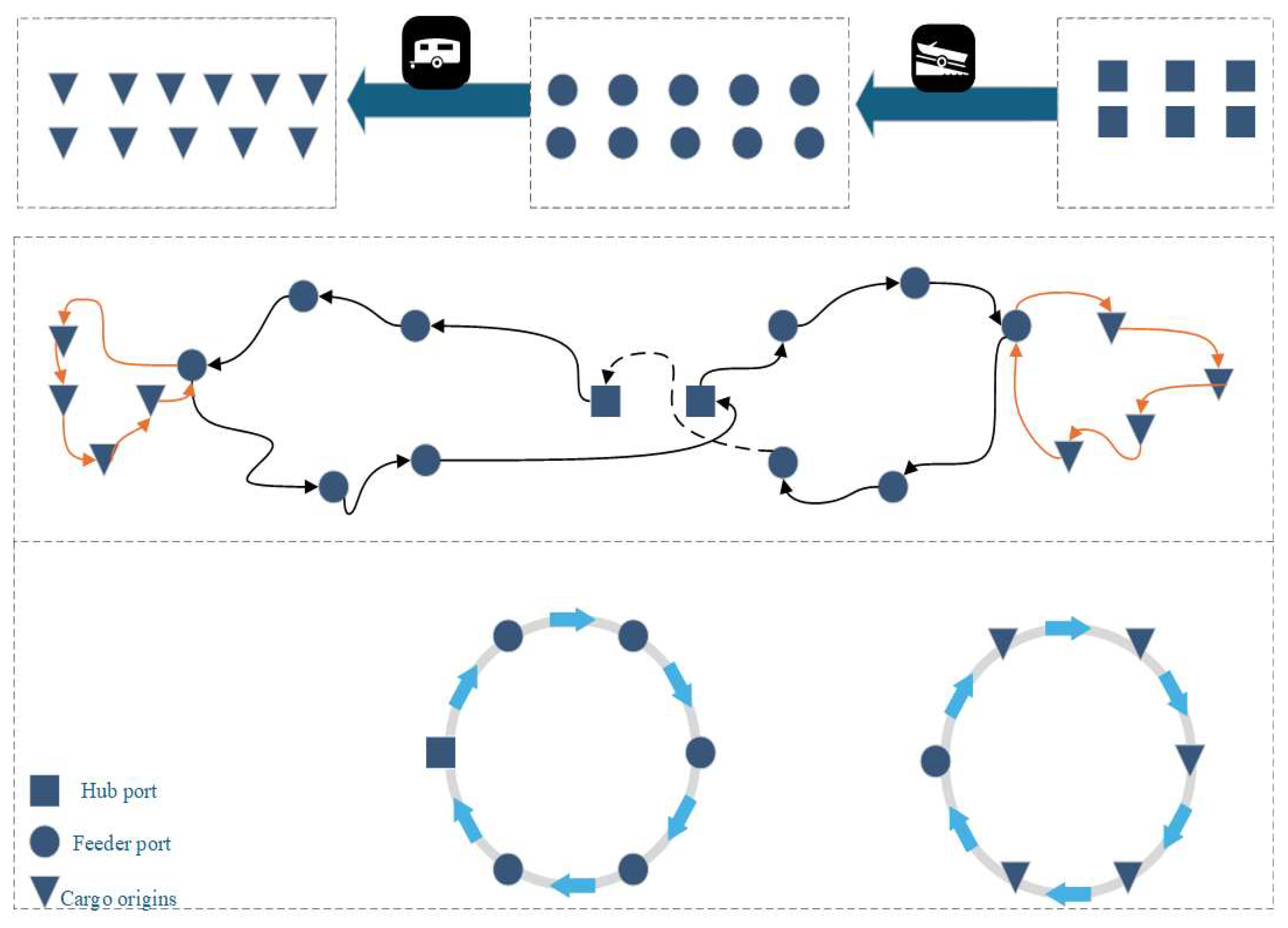
Disclaimer/Publisher’s Note: The statements, opinions and data contained in all publications are solely those of the individual author(s) and contributor(s) and not of MDPI and/or the editor(s). MDPI and/or the editor(s) disclaim responsibility for any injury to people or property resulting from any ideas, methods, instructions or products referred to in the content. |
© 2025 by the authors. Licensee MDPI, Basel, Switzerland. This article is an open access article distributed under the terms and conditions of the Creative Commons Attribution (CC BY) license (https://creativecommons.org/licenses/by/4.0/).