Recent Developments in Cross-Shore Coastal Profile Modeling

Abstract

Coastal profile models are frequently used for the computation of storm-induced erosion at (nourished) beaches. Attention is focused on new developments and new validation exercises for the detailed process-based CROSMOR-model for the computation of storm-induced morphological changes in sand and gravel coasts. The following new model improvements are studied: (1) improved runup equations based on the available field data; (2) the inclusion of the uniformity coefficient (C_u = d₆₀/d₁₀) of the bed material affecting the settling velocity of the suspended sediment and thus the suspended sediment transport; (3) the inclusion of hard bottom layers, so that the effect of a submerged breakwater on the beach–dune morphology can be assessed; and (4) the determination of adequate model settings for the accretive and erosive conditions of coarse gravel–shingle types of coasts (sediment range of 2 to 40 mm). The improved model has been extensively validated for sand and gravel coasts using the available field data sets. Furthermore, a series of sensitivity computations have been made to study the numerical parameters (time step, grid size and bed-smoothing) and key physical parameters (sediment size, wave height, wave incidence angle, wave asymmetry and wave-induced undertow), conditions affecting the beach morphodynamic processes. Finally, the model has been used to study various alternative methods of reducing beach erosion.

1. Introduction

Coastal profile models are very useful tools for the assessment of the morphological behavior of relatively uniform and long-stretched beach–dune systems (none with only minor alongshore gradients of water levels, incident wave height, sand transport, etc.). Most generally, the focus is on the behavior of nearshore mounds and berms, beach and dune erosion due to storm events and the lifetime estimation of shoreface nourishments and beach fills. Basically, two types of coastal profile models can be distinguished [1]: (1) process-based models for short-term (<3 years) predictions and (2) semi-empirical parametric models for long-term (decadal) predictions.

Typical examples of process-based models are the UNIBEST-model developed at Deltares (Stive 1986 [2], Roelvink et al., 1995 [3]); the DUROSTA-dune erosion model (Steetzel, 1993 [4]); the COSMOS-model developed at HR Wallingford (Nairn and Southgate, 1993 [5]); the CROSMOR-model of LVRS-Consultancy (Van Rijn and Wijnberg, 1996 [6], Van Rijn, 1998, 2009, 2025 [7,8,9], Van Rijn et al., 2003 [10]); the CSHORE-model developed by Kobayashi and Farhadzadeh, 2008 [11]; and the XBEACH-model developed by Roelvink et al., 2009 [12], and McCall et al. [13], which is an open source model with continuous improvements. This latter detailed model includes a unique non-stationary wave driver with directional spreading to account for wave-group generated surf and swash motions (infra-gravity waves). Most of these models predict beach–dune erosion under breaking waves rather well but cannot accurately address the subsequent recovery of the beach profile (e.g., onshore bar migration) under relatively quiescent wave conditions. Ruessink et al., 2007 [14], studied the model parameter settings required to simulate onshore bar migration. Near-bed wave skewness affecting bedload transport was found to have a dominant effect, whereas the effects of bound infra-gravity waves and near-bed streaming were found to be negligible. Various studies show that the prediction of on/offshore bar migration in near-equilibrium morphodynamic conditions using process-based models requires an extensive (often site-specific) parameter calibration at the present stage of research [15,16,17,18].

Typical examples of parametric models are the DUROS and DUROS+-dune erosion models [19,20]; the Dean profile model [21]; and the SBEACH-model (Storm-induced BEAch CHange), which has been developed at the U.S. Army Engineer Waterways Experiment Station to calculate beach and dune erosion under storm water levels and wave action [22,23]. This model calculates the net cross-shore sand transport rate in four zones from the dune or beach face, through the surf zone and into the offshore based on the inputs of initial profile, grain size, water level and wave height data. The wave model includes wave shoaling, refraction, breaking, breaking wave re-formation, wave- and wind-induced setup and set-down and runup. Larson et al., 2016 [24], proposed another model (CS-model) that can better represent the bar, berm, beach and dune morphology. This model consists of modules for calculating dune erosion and overwash, wind-blown sand transport and bar–berm material exchange. The key parameters modeled are the dune height, the locations of the landward dune foot, seaward dune foot, berm crest and shoreline and the bar volume. Marinho et al., 2020 [25], and Romao et al., 2024 [26], improved the CS-model concept to be able to better simulate the behavior of bars, berms and artificial beach nourishments and coupled the model to a coastline evolution model. Diez et al., 2017 [27], presented and tested a parametric model that describes the equilibrium shape of the dry beach in the cross-shore direction, i.e., an equation for the dry beach equilibrium profile. The model has equations with shape parameters to describe the foreshore, berm and beach morphology. The shape parameters are related to the nearshore wave climate and the sediment characteristics. Kettler et al., 2024 [28], proposed a diffusion-based cross-shore model (Crocodile-model) for a better simulation of beach nourishments on decadal time scales. The key model parameters are the profile volume, coastline position, beach width, cross-shore diffusion, sediment exchange with the dune and longshore sediment losses.

In the period of 2000–2025, a special class of Machine Learning parametric models (ML tools) has come up: ML tools (for example, TOPOFORMER) with supervised deep learning algorithms/architecture (including memory layers and neural networks), in which preferred known patterns can be imposed by the user to better identify the spatio-temporal and often non-linear dependencies of the multiple key parameters of the coastal system and databases (forcing variables, beach characteristics, satellite data) [29,30,31]. Large databases are required for training the models involved, which generally are not available for most coastal sites. Furthermore, these types of models, similar to all parametric models, are very site-specific, lacking generality. Once properly calibrated for a particular site, parametric models are very suitable for the evaluation of long-term morphological trends, including the effects of sea level rise.

In this paper, the attention is focused on the new developments and new validation exercises of the detailed process-based CROSMOR-model for sand and gravel coasts. The new model improvements are as follows: (1) improved runup equations based on the available field data; (2) the inclusion of the uniformity coefficient (C_u = d₆₀/d₁₀) of the bed material affecting the settling velocity of the suspended sediment and thus the suspended sediment transport [32]; (3) the inclusion of hard bottom layers, so that the effect of a submerged breakwater on the beach–dune erosion can be assessed; and (4) the determination of adequate model settings for the accretive and erosive conditions of coarse gravel–shingle types of coasts (sediment range of 2 to 40 mm). The improved model has been extensively validated for sand and gravel coasts using the available field data sets. Most profile models can only be applied for short-term storm-related erosion, but the CROSMOR-model can also simulate long-term morphological changes due to both onshore and offshore sand transport processes for strongly disturbed coastal profiles with nourishments and/or structures. However, the prediction of natural bar migration close to dynamic equilibrium morphology remains (too) problematic at the present stage of research.

The CROSMOR-model and the improvements (bed material composition, hard layers, wave runup) are briefly described in Section 2. The effects of numerical parameters on model accuracy are studied in Section 3. Many new validation cases for sand and gravel coasts are extensively analyzed in Section 4. The effects of the key physical parameters on beach erosion based on many sensitivity runs are studied in Section 5. Finally, in Section 6, the model is used to study the effects of various alternative methods to reduce beach erosion. A summary, discussion and conclusions are given in Section 7.

2. Model Description and Improvement

2.1. General

The CROSMOR-model is a one-dimensional FORTRAN model [7,8,9,10] for the computation of hydrodynamic parameters and bed profile changes in a cross-shore direction for given offshore wave conditions. The model and new developments are briefly described in Section 2.2 and Section 2.3. The model accuracy and the effect of numerical parameters based on sensitivity runs are studied in Section 3.

2.2. Model Description

The morphodynamic CROSMOR2025-model is the most recent updated version, which can be used to compute the cross-shore profile distribution of wave heights, peak orbital velocities, undertow velocity, longshore currents, bed and suspended load transport and the bed profile development as a function of time. Earlier versions of the model have been extensively validated by [7,8,9,10].

The propagation and transformation of individual waves (wave by wave approach based on Rayleigh distribution) along the cross-shore profile are described by a probabilistic model solving the wave energy equation for each individual wave. The number of wave classes can be set by the user. The individual waves shoal until an empirical criterion for breaking is satisfied. The maximum wave height is given by H_max = γ_br h, with γ_br = breaking coefficient and h = local water depth. The default wave breaking coefficient is represented as a function of the local wave steepness and bottom slope. The default breaking coefficient varies between 0.4 for a horizontal bottom and 0.8 for a very steep sloping bottom. The model can also be run with a constant breaking coefficient (input value). Wave height decay after breaking is modeled by using an energy dissipation method. Wave-induced setup and set-down and breaking-associated longshore currents are also modeled. Laboratory and field data have been used to calibrate and verify the model.

The complicated wave mechanics in the swash zone are not explicitly modeled, but are taken into account in a schematized way (supra swash model). The limiting water depth of the last (process) grid point is set by the user of the model (input parameter; typical values of 0.1 to 0.3 m). Based on the input value, the model determines the last grid point by an interpolation after each time step (variable number of grid points). The wave runup is part of the supra swash model between the last grid point and the wave runup point.

The cross-shore wave velocity asymmetry under shoaling and breaking waves is described by semi-empirical methods. Similarly, near-bed streaming effects in the surf zone and low frequency velocities in the swash zone are modeled by semi-empirical methods.

The depth-averaged return current (u_r) under the wave trough of each individual wave (summation over wave classes) is derived from the linear mass transport and the water depth (h_t) under the trough. The contribution of the rollers of broken waves to the mass transport and to the generation of longshore currents is taken into account.

The sand transport, including slope effects, is based on the sand transport formulations proposed by Van Rijn, 2007 [33,34,35]. The sand transport rate is determined for each wave (or wave class), based on the computed wave height, depth-averaged cross-shore and longshore velocities, orbital velocities, friction factors and sediment parameters. The total sediment transport is obtained as the sum of the net bed load (q_b) and net suspended load (q_s) transport rates. The net bed load transport rate is obtained by time-averaging (over the wave period) the instantaneous bed–shear stress, including waves and currents and the corresponding transport rate in the wave cycle. The net suspended load transport is obtained as the sum (q_s = q_s,c + q_s,w) of the current-related and the wave-related suspended transport components. The current-related suspended load transport (q_s,c) is defined as the transport of sediment particles by the time-averaged (mean) current velocities (longshore currents, rip currents, undertow currents). The second-order wave-related suspended sediment transport (q_s,w) is defined as the transport of suspended sediment particles by the oscillating fluid components (cross-shore orbital motion).

2.3. Model Improvements

2.3.1. Bed Material Composition and Hard Layers

Natural sand mixtures are inherently non-uniform, which means that the sand mixture consists of multiple sand fractions with slightly different particle sizes, as expressed by the particle size distribution (psd-curve). The basic parameters of the psd-curve are (1) the median particle diameter (d₅₀), (2) the uniformity coefficient (C_u = d₆₀/d₁₀) and (3) the grading coefficient C_c = (d₃₀)²/(d₆₀ d₁₀). Practice shows that finer sands are more uniform than coarser sands. Thus, the c_u-value increases for increasing median particle sizes. Very fine sands with d₅₀ < 0.2 mm generally have C_u-values < 2.5, and coarser sands with d₅₀ of about 0.5 mm generally have C_u-values ≅ 3.

So far, the bed was assumed to consist of uniform sediment in the CROSMOR-model. This means that the sediment in suspension (and settling velocity) is the same as that of the bed material, which is reasonably correct for storm conditions, but not for daily wave conditions. In daily conditions with lower waves, the finer sediments are washed out first from the bed material, resulting in finer suspended sediments and lower settling velocities. This effect can now be included by a function [32] which predicts the suspended sediment size (d_s) as function of the d₅₀, the C_u-coefficient and the wave conditions. For increasing wave conditions, the d_s of the suspended sediments gradually approaches the d₅₀ of the bed material.

Another model improvement is the inclusion of hard layers to represent a structure (submerged, shore-parallel breakwater) near the coast. Sediment can be deposited on the hard layer and eroded as long as sediment is present on the hard layer. In erosion conditions with no sediment present on the hard layer, the sediment transport remains constant above the structure.

2.3.2. Wave Runup Equations

Wave runup and swash are extremely important for beach erosion. Since the development of the CROSMOR-model around 2000, more laboratory and field data on runup have become available, and therefore the existing wave runup equation has been re-evaluated.

Wave runup and beach erosion mainly take place in the upper swash zone where water and sand are moved from the upper beach and dune towards the lower parts of the intertidal and subtidal beach. One single storm event can move large quantities of sand up to 300 m³/m/event away from the beach. A typical phenomenon is the generation of erosion cliffs at the upper beach, particularly for gravel beaches, but they also are present at nourished sand beaches after minor storms. The swash zone is the zone which is intermittently wet and dry, showing relatively large velocities during the uprush and backwash phases of the saw-tooth swash wave cycle due to bore propagation and bore collapse, often in combination with low-frequency oscillations which generally grow in amplitude towards the shoreline. It is a particularly complex nearshore zone where short and long waves, tides, sediments and groundwater flow (infiltration/percolation) all play an important role. Long waves are generated in the surf zone due to the release of bound long waves during the breaking process of short waves and by cross-shore variations in the short wave breakpoints (surf beat). The role of percolation is especially important on steep, coarse-grained beaches, leading to beach accumulation and steepening as a result of the diminished sediment-carrying capacity of the reduced backwash volume of water and velocity, following percolation into the coarse-grained bed. These effects will lead to a landward bias (asymmetry) in swash transport depending on grain size. The swash zone is the most dynamic part of the nearshore zone and is of vital importance for the behavior of sand and gravel beaches.

In Section 2.3.3, a brief summary of the most relevant wave runup equations for mild and steep beaches is given focusing on the available field data, which have been used to derive a new general runup equation for the CROSMOR-model, as described in Section 2.3.4.

2.3.3. Wave Runup Equations

Very basic to all profile models is the description of the wave runup across the beach and dune front. Dune and beach morphology strongly depends on the wave runup in addition to the wind-induced setup (surge).

Generally, the wave runup for irregular waves is expressed as R_2%, which is the runup exceeded by 2% of the waves. On average, the total wave runup above the still water level (SWL) consists of contributions of wave-setup (about 25%) and runup (about 75%). This latter runup consists of high-frequency (T < 20 s) and low-frequency contributions (T > 20 s; known as infra-gravity contributions).

Three types of relationships are used to describe the total wave runup, as follows:

• R_2% = αH_s,o; wave runup only depends on the offshore wave height H_s,o;
• R_2% = α(H_s,o L_s,o)^0.5 = α[H_s,oT_p²g/(2π)]^0.5; effect of the wave period is included;
• R_2% = αζ_oH_s,o; effect of the wave period and beach slope are included (ζ_o = tanβ/(H_s,o/L_s,o)^0.5, with tanβ = beach slope around water line).

Guza and Thornton, 1982 [36], analyzed the field data on wave runup in the USA and derived a simple expression:

R_2% = 0.035 + 0.71 H_s,o

(1)

which is independent of the beach slope. Some researchers (Douglass, 1992 [37]; Nielsen and Hanslow, 1991 [38]) have questioned the dependence of wave runup on the beach slope. Douglass, 1992 [37] analyzed the runup data of natural beaches and argued that the beach slope is not an important parameter for predicting wave runup on natural beaches. Given the problem of defining beach slope and the slope variability, Douglass suggested that beach slope can be eliminated from the runup equation.

Stockdon et al., 2006 [39], analyzed the wave runup data (with 0.1 < ζ_o < 2.5) of ten different field experiments (west and east coasts of USA and the coast of Terschelling Island of The Netherlands) based on video techniques. Their equation is described as follows:

R_2% = 0.043 [H_s,o L_s,o]^0.5 = (0.043/tanβ) H_s,o ζ_o for ζ_o < 1 (dissipative beaches)

(2a)

R_2% = 0.75 (sinβ)[H_s,oL_s,o]^0.5 ≅ 0.75 H_s,o ζ_o for ζ_o > 1 (reflective beaches)

(2b)

with H_s,o = the significant wave height in deep water.

Senechal et al., 2011 [40], performed field experiments in March–April of 2008 at the barred surf and beach zone of the Truc Vert site (sand 0.35 mm) on the Atlantic coast of France. Video measurements of wave runup were collected during extreme storm conditions, characterized by energetic long swells (peak period of 16.4 s and offshore wave heights up to 6.4 m) impinging on relatively steep foreshore beach slopes (0.06–0.08). The measured ζ_o-values are in the range of 0.5 to 0.9. Their observations show that the total vertical wave runup is dominated (75%) by the infra-gravity components with periods > 20 s. The highest measured runup value was about 2.5 m for an offshore wave height of 5 m (ζ_o = 0.58; tanβ = 0.069). They also found that the infra-gravity component becomes saturated (percentage of low frequency waves does not increase anymore) for offshore significant wave heights above 4 m. For minor storms with H_s,o < 4 m; the total wave runup can be represented as 0.6H_s,o, which is close to the runup Equation (1) of Guza and Thornton, 1982 [36]. The effect of the beach slope on the wave runup was not found to be very important (weak effect). The total wave runup data, consisting of high- and low-frequency contributions, of Senechal et al., 2011 [40], are herein represented by the following:

R_2% = α_s (ζ_o)^0.6 H_s,o; with α_s = 0.9 (best fit) and α_s = 1.15 for upper envelope

(3a)

R_2% = α_s[H_s,oL_s,o]^0.5 = α_s[H_o T_p² g/(2π)]^0.5

(3b)

with α_s = 0.06 (best fit) and α_s = 0.075 for upper envelope.

Equation (3b), which is plotted in Figure 1, is close to the wave runup Equation (2b) of Stockdon [39]. Clearly, the runup values for natural sand beach slopes are much smaller (factor 2) than those of impermeable slopes (Mase, 1989 [41], and Van Gent, 2001 [42]) for the same value of the surf similarity parameter, mainly due to the effects of beach permeability, nonuniform slope, wave breaking over bars and other factors (Hughes, 2004 [43]).

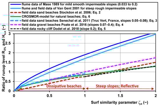
Figure 1. Dimensionless runup R_2%/H_s,o as function of the surf similarity parameter ζ_o [39,40,41,42,44,45].

Poate et al., 2016 [44], have studied the wave runup at gravel–shingle beaches at six sites in the UK (H_s,o = 2 to 6 m; tanβ = 0.07 to 0.4; d₅₀ = 2 to 160 mm; ζ_o = 0.5 to 5). At each site, the wave runup was measured using video data. Nearshore wave data were measured by directional waveriders at a depth of −10 m CD. The deep-water wave height (H_s,o) was obtained by de-shoaling the nearshore significant wave height using the spectral mean wave period for a 200 m water depth. The highest runup value of 12.5 m for an offshore wave height H_s,o = 6.5 m was measured at the very steep Chesil gravel barrier (d₅₀ = 40–50 mm; tanβ = 0.4 or 1 to 2.5; ζ_o ≅ 3; R_2%/H_s,o ≅ 2). The R_2% values can be roughly represented by the following:

R_2% = α (ζ_o)⁰.⁸ H_s,o with α = 1 (best fit) and α = 1.5 for upper data envelope

(4)

Equation (4) is shown in Figure 1 and Figure 2.

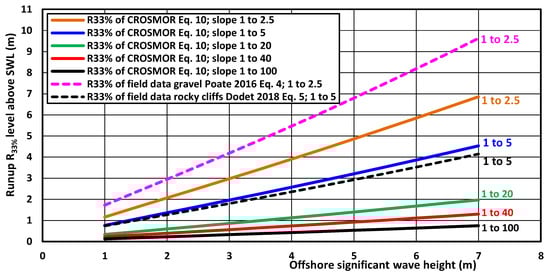
Figure 2. Runup levels (R_33%) above still water level (SWL) [44,45].

Dodet et al., 2018 [45], have studied the wave runup over steep impermeable rocky cliffs (October 2012 to May 2015) at Banneg Island, Brittany, France, in conditions with a tidal range of 2 to 8 m. The beach slope between LAT and HAT (distance of about 50 m) was tanβ = 0.2. The offshore wave rider buoy was at a 50 m water depth, 1 km from the shore. Four pressure sensors were deployed in the LAT-HAT zone. The highest sensor P4 was at 1.6 m above HAT. The η_2–value was measured, which is the 2% exceedance of the water level elevation above the still water level (SWL) of the highest pressure sensor P4. This η_2%-parameter is somewhat lower than the R_2%-parameter. The highest measured η_2%-value was 5.4 m in 131 events for H_s,o ≅ 4.5 m. The η_2%-values of sensor P4 for a cliff slope of tanβ = 0.2 can be roughly represented by the following:

η_2% = α (ζ_o)^0.8 H_s,o with α = 0.75 (best fit) and α = 0.9 for upper envelope

(5)

Equation (5) is shown in Figure 1 and Figure 2. Equation (5) for steep cliffs gives somewhat lower values (30%) than Equation (4) for gravel beaches. For natural steep rocky cliffs, the runup dynamics are more complex, with a higher reflection due to increased steepness, stronger dissipation due to increased drag over an irregular bottom, enhanced turbulence during the breaking processes affected by impacts, splash-ups and air entrapment and the volume loss of the swash tongue due to infiltration within fractured bed rock.

2.3.4. Wave Runup Equation of CROSMOR-Model

Analyzing all available runup data, the standard runup equation in the CROSMOR-model is described as follows (accuracy of 30%):

R_2% = 0.85 (ζ_o)^0.6 H_s,o

(6a)

R_33% = 0.7 R_2% = 0.6 (ζ_o)^0.6 H_s,o

(6b)

Equation (6) is only valid for natural sand beaches and is in good agreement with the runup values of Equation (3b), see Figure 1. It is noted that the beach erosion in the CROSMOR-model is based on R_33% (default setting), which is smaller than the R_2% (R_33% ≅ 0.7R_2%). The R_33%-value is most representative for the beach changes in the majority of the waves, while the R_2% is most important for dune crest overtopping by the most extreme wave heights. The model user can also apply the R_2%-value (frunup input parameter should be set to 1.4). A smaller runup value leads to a shorter wet beach length exposed to erosion (length between the last grid point and the runup point) and thus to a deeper erosion depth at the beach. All flume and field data in terms of the ζ_o-parameter are shown in Figure 1. The most striking results are the following:

• The wave runup values for the sand beaches of Stockdon et al., 2006 [39], are somewhat smaller than those of Senechal et al., 2011 [40]; the CROSMOR values are closest to the values of Senechal et al., 2011 [40];
• The wave runup values for steep gravel beaches are higher (30%) than at sand beaches; the wave runup values for rocky cliffs are much lower than at gravel beaches, but are reasonably in agreement with the CROSMOR equations for wave runup;
• The wave runup values for the mild and steep, smooth, impermeable slopes of Mase, 1989 [41], and Van Gent, 2001 [42], are much higher (factor 1.5 to 2) than those at gravel beaches.

Figure 2 shows the computed runup levels of Equation (6) in terms of R_33% (R_33% ≅ 0.7 R_2%) as function of the offshore wave height, H_s,o = 1 to 7 m (T_P = 6 to 12 s), for beach slopes of 1 to 1/10/20/40/100. The results of the field data using Equation (4) of Poate et al., 2018 [44], for gravel beaches and Equation (5) of Dodet et al., 2018 [45], for rock slopes are also shown. The most striking features are the following:

• The wave runup of Equation (6) of the CROSMOR-model is relatively small (about 1 m for H_s,o = 7 m) for mild slopes between 1 and 100 and 1 and 40;
• The wave runup of Equation (6) increases to 2 m for a slope of 1 to 20, to 4 m for a slope of 1 to 5 and to 7 m for a slope of 1 to 2.5 in the case of H_s,o = 7 m;
• The wave runup values for cliff and gravel slopes are relatively high and reasonably represented by the CROSMOR Equation (6) for slopes up to 1 to 5; Equation (6) underpredicts for steep gravel slopes (1 to 2.5).

3. Model Accuracy and Numerical Behavior

The accuracy of the bed evolution is strongly influenced by the grid size (DX), the time step (factime) and the bed-smoothing parameters (facsmooth, sw), particularly for long-term computations. Short-term computations for storm erosion on the time scale of a few days generally are quite accurate. Bed-smoothing is applied at each time step for reasons of computational stability for long-term time scales (years). The bed level in the main computational domain is smoothed by the facsmooth coefficient, while the bed level in the supra swash zone is smoothed by the sw coefficient. It is noted that, in nature, substantial smoothing may occur due to horizontal water circulation in the surf zone.

The bed-smoothing in the computational domain is part of the bed level computation method based on the explicit Lax–Wendorf scheme [9], which reads as follows:

z_b,i,t+Δt = z_b,i,t − γ Δt/(2Δx) [S_i+1,t − S_i−1,t] + α[z_b,i+1,t − 2z_b,i,t + z_b,i−1,t]

(7)

with: z_b = bed level (m) to a datum at location x and at time t; S = q_b,x + q_s,x = bed load transport plus suspended load transport (kg/m/s); γ = 1/((1 − p)ρ_s) = coefficient, where p = porosity factor of bed material and ρ_s = sediment density (kg/m³); Δt = time step; Δx = horizontal grid size; and α = smoothing coefficient (including facsmooth coefficient).

The most optimum values of DX, factime, facsmooth and sw can only be determined by trial and error through a series of runs with a systematic variation in these parameters. It is best to start with a small time step and grid size and relatively high smoothing parameters, which are then systematically adjusted to obtain stable and accurate results.

The grid size is particularly important for the steep bed sections, where the grid size should be in the range of 0.5 to 2 m. The time step should be as small as possible (factime in range of 0.5 to 2; default = 1), but it should be realized that a smaller time step also means that the bed-smoothing procedure is applied more often. The bed-smoothing parameter should also be as small as possible (facsmooth in range of 5 to 15; default = 10). Facsmooth values smaller than 5 may easily lead to bed level instability and model failure; facsmooth values larger than 15 may result in inaccurate results.

The model accuracy is tested for a very complex profile of a land reclamation site with a rather steep bed section of 1 to 5 between x = 3300 m and 3345 m, in combination with an excessive wave height of H_s,o = 10.5 m in the wave climate. The beach landward of x = 3345 m also has a relatively steep slope of 1 to 20. The dune crest lies at 5 m above MSL. The schematized annual wave climate consists of four wave conditions, with H_rms,o = 0.35, 1.0, 2.1 and 3.5 m, and one extreme storm of H_rms,o = 7.45 m (H_s,o = 10.5 m, T_p = 13 s). The offshore wave incidence angle is 5° to the shore normal for all conditions. This case is a very severe test of the CROSMOR-model for a beach with very steep slopes and high waves. The input data for a long-term run over 730 days are given in Table 1.

Table 1. Input data of CROSMOR-model.

Input Parameters	Parameter Abbreviation	Values
Tide water level Tidal current (longshore, cross-shore)	WS VNUL1; VNUL2	−0.15, +0.15 m; 0.1; m/s
Bed profile to MSL (m)	HMSL	−50 m at deep water to +5 m at dune crest
Number of grids along profile	NSTAP	0 to 100
Storm level above MSL (m)	HSTORM	0 to 2 m
Maximum dune slope SL	SL	50° (sliding if slope is larger)
Boundary depth near beach (m)	HGRENS	0.3 m (last grid point)
Grid size (m)		20 m offshore; 1 m nearshore
Profile of hard layer to MSL (m)	HRMSL	None
Number of wave classes per wave height	NHW	1
RMS-wave height, period and wave incidence angle at deep water	HRMS, T, THETA	Hrms = 0.35 to 7.45 m (Hs,o = 0.5 to 10.5 m); Tp = 7 to 13 s, angle = 5°
Wave asymmetry method	SWIT1	Isobe-Horikawa 1982 [46]
Wave breaking (−); roller coefficient (−)	GAMMA CRL	0 (automatic); 0.5
Runup coefficient (−)	FRUNUP	0.5 (default = 1)
Coefficients wave averaging for undertow and longshore current	COEF6 COEF5	3 for field; 1 laboratory cases 3 for field; 1 laboratory cases
Longuet–Higgins streaming (−);	CLH	0.5 (default = 1)
Grain diameter sand d50 (m) Cu-coefficient (−)	D50 CU	0.45 mm; 2
Coefficients sand transport formulas facbed; facsus; facsusw (−)	FACBED FACSUS FACSUSW	0.7; 0.7; 0.3 (default 1)
Coefficient extra sand entrainment in dune zone	SEF	1 (default = 1; range 1–2)
Coefficient bed concentration landward of hard layer (−)	FSAND	1 (default)
Coefficient undertow (−)	FRIP	1 (default)
Bed roughness (m)	KS	0 (automatic)
Bed smooth factors (−)	FACSMOOTH SW	30 (default = 10); 0.05 (default = 0.05)
Time step factor (−)	FACTIME	1 (default = 2)
Temperature (°C); Salinity (promille)	TE; SA	10 °C and 30 promille
Files		case3.inp; case3-k.inp

The following input parameters have been varied for this case:

• Grid size: The accuracy can be improved by reducing the grid size from 1 m to 0.5 m at the steep section x = 3300 to 3345 m; see Figure 3;
  

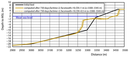  Figure 3. Effect of grid size.
• Time step and bed-smoothing parameters (factime and facsmooth): The effect of bed-smoothing can be seen at point x = 3000 where the sediment transport is very small and the deposition is mainly caused by the bed-smoothing procedure; the most accurate run is for factime = 2 and facsmooth = 5; see Figure 4; the run with factime = 1 and facsmooth = 5 has a lower smoothing coefficient but the smoothing procedure is applied more often due to the smaller time step (factime = 1), which leads to more smoothing of the bed;
  

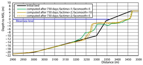  Figure 4. Effect of time step (factime) and bed-smoothing parameter (facsmooth).
• Effect of bed-smoothing in the swash zone (sw): sw = 0.005 and 0.01 instead of sw = 0.05 gives somewhat more erosion because less smoothing is applied; sw = 0.01 is sufficiently accurate; see Figure 5; slight instability (minor saw-tooth pattern) along the bed can be seen between x = 3275 and 3300 m; the bed comes unstable for SW < 0.005 (run breaks off).
  

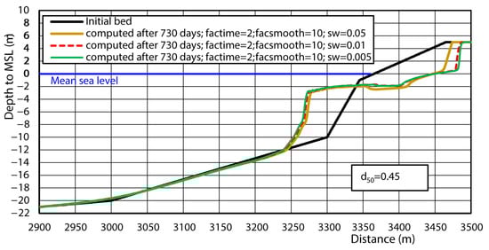  Figure 5. Effect of bed-smoothing parameter (sw).

4. Model Validation for Sand and Gravel/Shingle Beaches

4.1. Model Validation Sand Beaches

The CROSMOR-model has been validated earlier based on dune erosion experiments in a large-scale wave flume [8,9]. Reliable field data were not available at that time. Now, the focus is on additional accurate field data of beach–dune erosion at sites in Belgium [47,48,49] and in The Netherlands [50]. Recently, two test dunes have been constructed and monitored [50] during the storm season at the Sand Motor site in The Netherlands. These field data have been used for a more detailed validation of the CROSMOR-model.

The Brier Skill Score BSS [10] is used to express the model performance. The BSS-parameter compares whether the computed bed profile at time t is closer to the measured bed profile at time t than the initial profile of t = 0. BSS = 0.8–1 = excellent; BSS = 0.6–0.8 is good; BSS = 0.3–06 = fair/reasonable; and BSS < 0.3 = poor.

4.1.1. Beach–Dune Erosion of Test Dunes at Site Sand Motor, The Netherlands

In the winter period of October 2021 to March 2022, two test dunes of sand (d₅₀ ≅ 0.3 mm) have been constructed and monitored along the coastline of the Sand Motor site in the south-west part of the Holland coast (Van Wiechen et al., 2022 [50]). The crest of the dunes is at +5 m NAP (Dutch Ordnance Datum ≅ −0.1 m below MSL). Dune 2 has a slightly different orientation, with more oblique incoming waves. Three minor storm events with maximum offshore significant wave heights of H_s,o,max = 3.04 m (T_p = 8.3 s), 4.27 m (T_p = 9.5) and 4.03 m (T_p = 9.6 s) occurred in the period from 6 November 2021 to 6 January 2022. The offshore wave incidence angle to the shore normal was about 10° for Dune 1 and 20° for Dune 2 to the local shore normal. Herein, it is assumed that each storm consists of 6 h with H_s,o = 0.5H_s,o,max, 3 h with H_s,o = H_s,o,max and 3 h with H_s,o = 0.5 H_s,o,max (total duration 3 × 12 = 36 h). The local tidal range is about 2 m. The maximum water level was about 2.2 m (storm setup of about 1.5 m). The most important model settings for both cases are the following: facbed = 0.5, facsus = 1.1, SEF = 2; slope angle dune front SL = 50°. Figure 6 and Figure 7 show measured and computed bed profiles before and after the storm period. All measured data are shown (x > 7100 m and >7140 m). Quite a good agreement can be observed. The computed and measured dune erosion is about 23 m³/m. The Brier Skill Score [10] is 0.9 for Dune 1 and 2, which means an excellent hindcast prediction.

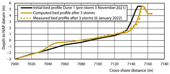
Figure 6. Measured and computed beach–dune profiles for Test Dune 1 at Sand Motor site.

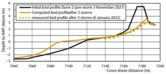
Figure 7. Measured and computed beach–dune profiles for Test Dune 2 at Sand Motor site.

4.1.2. Beach–Dune Erosion at Site De Haan, Belgium

Between 25 January and 1 March of 1990, the coast of Belgium was hit by a record number of storms, with maximum wind gusts up 165 km/h in a period of just over a month. The effective storm period with the highest waves is 5.5 days. The coastal damage was substantial along the entire coastline of about 60 km. The retreat of the dune profile at the beach village of De Haan due to the storms was measured in March 1990 [47,48,49]; see Figure 8. The maximum dune retreat is about 7 m and the total eroded volume is about 85 m³/m. The CROSMOR-model was applied for a storm period of 5.5 days with a maximum wave height of between H_rms,o = 1.1 and 3.4 m (H_s,o = 1.55 to 4.8 m; T_p = 4.3 to 7 s, wave angle = 5°; file case2m.inp). The tidal range is about 4.5 m. The sediment size is d₅₀ = 0.23 mm. The key model settings are as follows: SEF = 1.5; facbed = 0.5, facsus = 1.0. The computed beach–dune profile is in good agreement with the measured profile; see the upper part of Figure 8. The Brier Skill Score [10] is 0.82, which means an excellent hindcast prediction. This case has also been used for Monte Carlo simulations (20 runs). The following parameters have been varied: d₅₀ ± 15%; C_u ± 15%; SEF ± 15%; facbed ± 55%; facsus ± 15%. Each set of these five parameters has been selected by random number generation from the given variation range. The lower part of Figure 8 shows the computed bed profiles: the average profile and the average ± 1 standard deviation profiles. The average bed profile (red) is close to the bed profile computed with the mean parameter values (yellow). Many more runs (about 100) are required for a perfect match. The total erosion can be expressed as 85 ± 40 m³/m after the storm period, with an uncertainty of ±50%. This order of uncertainty is quite normal and acceptable for complex morpho-dynamic simulations in the coastal zone.

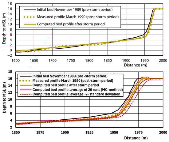
Figure 8. Measured and computed beach–dune profiles for storm period 1990, De Haan.

4.1.3. Beach–Dune Erosion at the Site HBZ Petten, Netherlands

Before 2015, the coastal section from Petten to Camperduin of the Holland coast was protected by an asphalt-type dike over an alongshore distance of about 6 km. Around 2015, a new natural sand dune was constructed in front of the dike. As this section was protected since 1600, while the adjacent coastal sections suffered from chronic erosion and retreat, the new sand dune protrudes into the sea over a distance of about 200 m with respect to the adjacent coastlines. This leads to erosional losses requiring regular maintenance nourishment. The CROSMOR-model has been used to estimate the erosion losses at profile km 25. The long-term annual wave climate is schematized into eight wave conditions, with H_s,o between 1.5 and 3.2 m, and one storm condition, with H_s,o = 5 m and duration of 12 h (file HBZ25.inp). The storm represents an event with a recurrence period of 5 years, which is applied each year over the computation period of 3 years (conservative approach). The vertical tide is between +1 and −0.8 m NAP. The maximum flood/ebb velocities in deep water are set to 0.3/0.25 m/s. The median sand size is d₅₀ = 0.3 mm. The measured bed profile at km 25 of 2015 is used as the initial construction profile, which has a flat beach at +2 m over 100 m (Rijkswaterstaat, JARKUS-database [51]).

Figure 9 shows the measured and the computed bed profiles after 3 years. The computed erosion volume landward of x = 1900 m is about 300 to 330 m³/m after 3 years, which is in reasonable agreement with the measured value of 340 m³/m. However, the computed erosion profile shows more erosion in the upper beach zone (x > 2200 m) compared to the measured profile. The eroded sediments are deposited in the bar trough zone at x = 1900 m, which is not observed in nature. This is caused by the relatively strong longshore current around the new protruding sand dune, which continuously removes the deposited sediments in the bar trough zone, carrying it along the coast. This 3D mechanism is absent in the 2D model, which has a closed sand balance in cross-shore direction. The measured profile only shows erosion without deposition (no closed sand balance). Nevertheless, the CROSMOR-model predicts a reasonable erosion loss from the new sand dune, which can be used to estimate the maintenance volume and re-nourishment cycle time. The Brier Skill Score [10] is 0.55 (fair/reasonable) without the bar trough area.

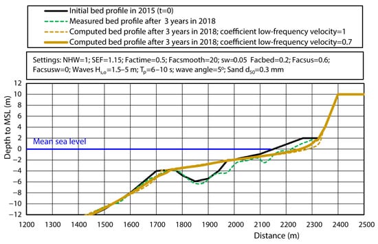
Figure 9. Measured and computed bed profiles, km 25, North Holland, The Netherlands.

4.2. Model Validation Gravel/Shingle Beaches

The new CROSMOR version 25 August 2025 has also been used to study the erosion of gravel–shingle gravel beaches. Beaches of gravel–shingle material generally extend down to −2 depth below MSL; seaward of this depth line, the bed usually consists of sandy sediments. This composite situation can also be modeled by the CROSMOR-model.

To justify that the CROSMOR-model produces realistic results for steep gravel beaches, four cases have been studied:

• Gravel transport rates in a unidirectional flow (river flow) computed by the CROSMOR-model (in river mode) are compared to the measured values of the gravel flume experiments of Meyer-Peter and Mueller, 1948 [52];
• Gravel longshore transport rates of the CROSMOR-model are compared to the measured longshore gravel transport at two field sites (Shoreham and Hurst Castle Spit [53,54]);
• CROSMOR simulation runs are made for gravel profiles in large-scale wave flumes;
• CROSMOR simulation runs are made for coastal gravel beach profiles at the field sites of Chesil beach (UK) and at Slapton Sands beach (UK).

4.2.1. Measured Bed Load Transport Rates of Gravel in Unidirectional Current

Very relevant for coastal gravel transport are the flume experiments of Meyer-Peter and Mueller, 1948 [52], with relatively large water depths in the range of 0.5 to 1 m. Gravel of 28.7 mm was tested in a wide flume (2 m). Gravel of 5.2 mm was tested in a small-scale flume (0.35 m). The initiation of motion starts at a velocity of about 1.8 m/s; see also Figure 10. The transport of gravel with d₅₀ = 28.7 mm is relatively low (<0.03 kg/m/s) for a current velocity of about 2 m/s. The transport rate of gravel increases to about 8 kg/m/s for a current velocity of 3 m/s. These results show that peak velocities of 2 to 3 m/s are required to produce the intensive transport of gravel in the coastal zone. Most likely, the gravel transport in field conditions is somewhat smaller than that in ideal flume conditions. Limiting factors in field conditions are wider size ranges and local armoring effects.

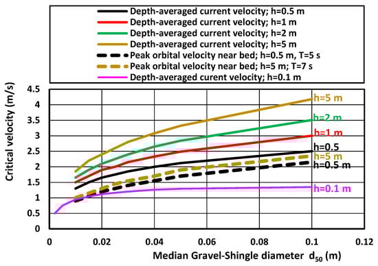
Figure 10. Initiation of motion for coarse (gravel) materials.

Figure 11 shows the measured bed load transport values (assumed error range of ±50%) as a function of the depth-averaged current velocity. Other measured values [36] are also shown. To show that the sediment transport equations of the CROSMOR-model can also be used to simulate gravel transport as measured in [52], the CROSMOR-model has been used in river mode (no waves; input file gravelr.inp) for a channel with a gravel bed.

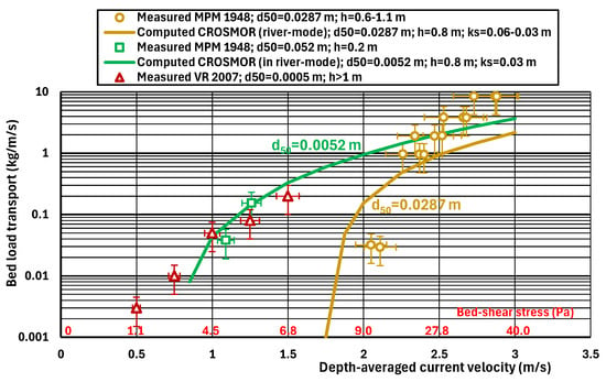
Figure 11. Measured and computed bed load transport rates for coarse sediments.

In the model run with gravel of 5.2 mm, the water depth was increased to take the side wall roughness of the small flume into account, resulting in a lower bed–shear stress and lower bed load transport. The bed roughness was set to k_s = 0.03–0.06 m to represent the bed form roughness. The computed bed load transport values are somewhat too small (factor of 2) for gravel of 28.7 mm, which can easily be calibrated. The effect of the sediment size decreases with increasing current velocity. Overall, the agreement between the measured and computed values is quite reasonable.

4.2.2. Measured Longshore Gravel Transport Data at Shoreham and Hurst Castle Spit, UK

Measured longshore transport data for gravel/shingle at field sites are rather scarce. Herein, measured data from two sites in the UK are used (Figure 12): Shoreham (Chadwick, 1989 [53]) and Hurst Castle Spit (Nicholls and Wright, 1991 [54]). A schematized cross-shore profile has been used in the model. The beach with d₅₀ = 20 mm has a steep slope of 1 to 8. The shoreface has a slope of 1 to 20. The tidal range is 4 m. The offshore significant wave height H_s,o is varied in the range of 0.7 to 8 m (H_rms,o = 0.5 to 5.7 m). The bed roughness values are taken equal to the median grain sizes (k_s = d₅₀).

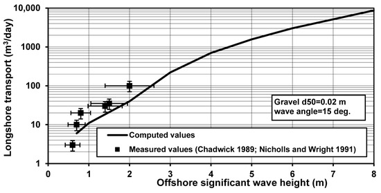
Figure 12. Measured and computed longshore transport as function of offshore wave height [53,54].

Figure 12 shows the measured and computed values (in m³/day) of the longshore transport integrated over the surf zone of the cross-shore profile. The computed model values vary roughly between 5 m³/day and 9000 m³/day (including pores). About 70% of the longshore transport occurs in the surf zone landward of the −4 m depth line. The computed longshore transport rates (in m³/day) for coarse gravel/shingle of 20 to 32 mm roughly are a factor of 2 to 3 too small for low wave conditions. This confirms that the CROSMOR-model underpredicts coarse gravel conditions (d₅₀ > 20 mm).

4.2.3. CROSMOR Simulation Runs for Coastal Gravel Profiles in Large-Scale Wave Flumes

Various experiments on the behavior of gravel and shingle beaches have been performed by Deltares, 1989 [55], in the large-scale Deltaflume. The gravel sizes were d₅₀ = 4.8 mm and d₅₀ = 21 mm. The initial beach slope was 1 to 5 (plane sloping beach) in all experiments. Similar experiments have been performed in the large-scale GWK flume in Hannover, Germany (López et al., 2006 [56]). The shingle material was d₅₀ = 20 mm. The initial slope of the beach was 1 to 8. In June and July 2008, large-scale experiments on gravel barriers (d₅₀ = 11 mm) were performed in the Deltaflume (Buscombe et al., 2008 [57]). The test results with a constant sea level show the formation of a typical swash bar landward of the still water level.

The most characteristic features observed in these flume tests are the following:

• The formation of swash bar above SWL (up to 2.5 m) due to onshore transport; see Figure 13; the swash bar extends substantially above SWL, indicating the effect of wave runup; the bar size increases with increasing wave height and increasing wave period;
  

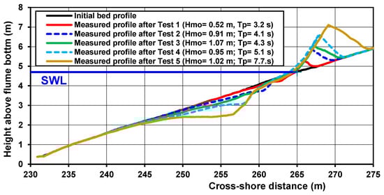  Figure 13. Measured bed profiles of shingles (d₅₀ = 0.02 m); accretive waves; GWK flume.
• The generation of a scour pit below SWL; scour depth extends substantially below SWL;
• The formation of a small breaker bar (below SWL) for relative fine gravel (d₅₀ = 4.8 mm);
• The generation of ripples with length scales of 1 to 3 m and height scales of 0.1 to 0.4 m at the lower part of the fine gravel slope (d₅₀ = 4.8 mm).

The formation of the swash berm/bar (Figure 13) is strongly related to the wave uprush and downrush near the water line. The uprush, with velocities in the range of 1 to 2 m/s, is much stronger than the downrush due to the percolation of water through the porous gravel bed surface, resulting in a relatively strong velocity asymmetry in the swash zone and hence net onshore transport of gravel particles. The total accretion area for the profiles of Figure 13 is about 10 m³/m. The transport of shingles passing the water line is about 10/57,100 = 0.0000175 m²/s or 15 m³/m/day for H_m,o ≅ H_s,o= 1 m.

The measured bed profiles of two large-scale wave flume experiments have been used for validation of the CROSMOR-model under accretive conditions. The validation cases are as follows: Test 1 of the Deltaflume experiments and Test B3 of the BARDEX experiments, with H_rms,o = 0.55 m (H_s,o = 0.7 m; T_p = 5 s). The basic model settings are the following: hgrens = 0.25 m; NHW = 6; facbed = 1; facsus = 1; facsusw = 0; frip = 1; sef = 1; k_s = 2d₅₀. The measured and computed bed profiles for Test 1 are shown in Figure 14.

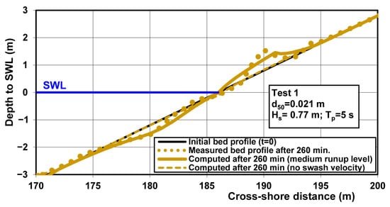
Figure 14. Measured and computed bed profiles for Test 1 of Deltalfume experiments.

In a qualitative sense, the results of the CROSMOR-model are in reasonable agreement with the measured values. A swash bar of the right order of size is generated above the waterline, but the computed swash bar is less peaked compared to the measured swash bar, which has a distinct triangular shape. The computed erosion zone is somewhat too large. The computed swash bar of Test 1 is much too small (only 0.05 m high) if the swash velocity is neglected in the model (C_sw = 0).

Figure 15 shows the simulation results of the CROSMOR-model for TEST B3 with H_rms,o = 0.7 m (H_s,o = 1 m, T_p = 5 s). The computed swash bar area is of the right order of magnitude (2 m³/m). The computed erosion volume is also of the right order of magnitude, but its position on the profile (below SWL) is much too low.

Figure 15. Measured and computed bed profiles for Test B3 of BARDEX experiments.

4.2.4. CROSMOR Simulation Runs for Chesil Gravel–Shingle Beach (UK)

Chesil beach on the south-west coast of the UK is a coarse shingle barrier (d₅₀ ≅ 40 mm) with the crest at approximately 12 m above OD (OD = Ordnance Datum Newlyn ≅ −0.2 m below MSL). This beach faces into the winter swells coming from the Atlantic Ocean. The tidal range is about 2 m. Offshore wave data have been measured by a directional wave buoy at a 12–15 m water depth at about 7 km from the beach. One storm event is considered: event CB02 from the data of McCall et al., 2015 [13]; see Figure 16.

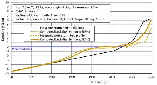
Figure 16. Measured and computed bed profiles for storm event CB02 of Chesil beach (UK).

Event CB02 is an extremely energetic event, with H_s,o = 7.6 m, T_p = 13.9 s. The morphodynamic impact on the beach backed by a seawall was very severe, with beach erosion of about 35 m³/m after about 22 h and deposition of sediment below MSL; see Figure 16. During this event, the beach profile changes were continuously measured by a tower-mounted laser scanner landward of the beach.

Figure 16 shows the measured and computed bed profiles for storm event CB02. The basic CROSMOR settings are as follows: NHW = 7, frunup = 1, facbed = 0.3, facsus = 3 (default = 1), facsusw = 0, frip = 3 (default = 1), slope = 50°, CLC = 1. The agreement between measured and computed results for these settings is quite good for SEF = 2 (Brier Skill Score = 0.85). The computed erosion is much too high for SEF = 3. The computed maximum undertow velocity in the nearshore zone for frip = 3 is about 2.25 m/s in the seaward direction. The setting facsus = 3 (default = 1) means that the offshore-directed sediment transport of coarse material had to increase substantially to obtain a good simulation result. Using the standard model settings, the sediment transport of very coarse material is underestimated, which was also found earlier (see Figure 11).

4.2.5. CROSMOR Simulation Runs for Slapton Sands Gravel Beach (UK)

Slapton Sand Beach on the south-west coast of the UK is a tidal beach with fine gravel (d₅₀ = 6 mm), with the crest at approximately 6.5 m above OD; see Figure 17. The initial slope is about 1 to 7 (slope angle of 8°).

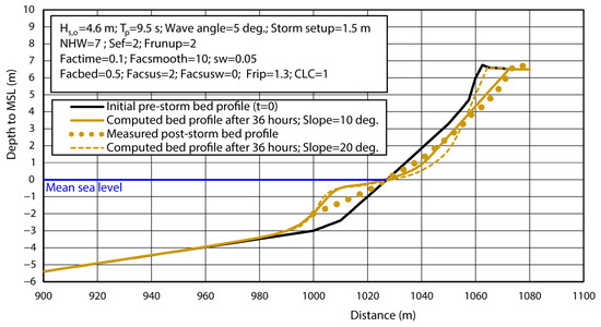
Figure 17. Measured and computed bed profiles for storm event SS02 of Slapton Beach (UK).

This beach is attacked by diffracted waves from the Atlantic Ocean and waves generated by local winds in the English Channel. The tidal range is about 2 m. Offshore wave data have been measured by a directional wave buoy at a 10–15 m water depth at about 0.5 km from the beach. One storm event is considered: event SS02 from the data of McCall et al., 2015 [13]. Event SS02 is a major storm event with H_s,o = 4.6 m, which resulted in severe beach erosion of 32 m³/m (crest was overtopped; crest retreat of 11 m) and a deposition of sediment at the toe of the beach.

Figure 17 shows the measured and computed bed profiles for storm event SS02. The basic CROSMOR settings are as follows: NHW = 7, frunup = 2, facbed = 0.5, facsus = 2 (default = 1), facsusw = 0, frip = 1.3 (default = 1), CLC = 1. The agreement between the measured and computed results for these settings is rather good (Brier Skill Score of 0.8) for a slope of 10°. The overall erosion volume is almost the same as the observed value (about 32 m³/m). However, the crest retreat of 11 m is somewhat underpredicted and the observed deposition is more seaward than predicted.

5. Model Sensitivity Tests; Effect of Key Physical Parameters

5.1. General

Based on the validation tests of Section 4, the parameter ranges of the model input are now better known. Using the case described in Section 3 (sand profile with d₅₀ = 0.45 mm), the effects of the key physical parameters on the bed profile changes are studied. The following parameters are considered:

• Representative wave height (number of wave classes);
• Wave height and wave incidence angle;
• Undertow, wave asymmetry (orbital velocities) and wave runup;
• Sand grain size and sand transport rates.

5.2. Effect of Representative Wave Height

A record of irregular non-breaking waves is mostly represented by the rms-wave height H_rms. Generally, the wave height of this record has a Rayleigh-type distribution, with higher and smaller waves. It is not, a priori, clear what the representative wave height is for sediment transport. The CROSMOR-model has been used to study this problem. Each wave height condition can be represented by either one (representative) wave height or by a series of Rayleigh-distributed waves. The number of Rayleigh wave classes to be used can be selected by the model user (input parameter NHW = 1 or NHW > 1).

If NHW > 1, the sediment transport is computed for each individual wave height and then summed over all wave heights, taking the frequencies of occurrence into account. It is noted that NHW > 1 is not very suitable for long-term runs because of excessive run times.

If NHW = 1, the representative wave height for sediment transport is set to H_{representative} = γ_rH_rms, with γ_r between 1 and 1.41 (set by model user). If γ_r = 1.41 is used, the significant wave height (H_s) is basically used as a representative wave height for sand transport.

Sensitivity runs with NHW = 1 have been made to assess the most appropriate γ_r-value compared to a similar run with NHW = 7. Two different cases are considered: 1) a storm with H_rms,o = 7.45 m (T_p = 14 s, θ_o = 10°, duration = 1 day) attacking a relatively steep beach profile of 1 to 5 between −10 m and −1 m and 2) a storm with H_rms,o = 3.55 m (T_p = 14 s, θ_o = 10°, duration = 2 day) attacking a relatively mild beach profile of 1 to 20 between −3 m and 0 m.

Figure 18 for case 1 shows that the computed beach erosion is substantially smaller for NHW = 7. Using NHW = 1, the γ_r-value should be set to 1 to have the best agreement with the profile for NHW = 7.

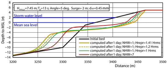
Figure 18. Effect of representative wave height (number of wave classes); storm case 1.

Figure 19 for case 2 shows that the computed beach erosion is somewhat larger for NHW = 7. Using NHW = 1, the γ_r-value should be set to 1.41 to have the best agreement with the profile for NHW = 7. Similar results were obtained for a run with d₅₀ = 0.25 mm and for a run with a lower wave height of H_rms,o = 2.12 m.

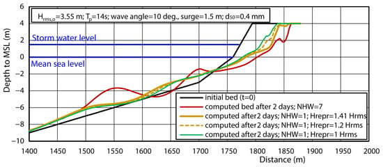
Figure 19. Effect of representative wave height (number of wave classes); storm case 2.

Based on these two cases, the type of bed profile (steep or mild slope) affecting the wave breaking processes has a significant effect on the most appropriate γ_r-value. The best approach for practical cases is to first determine the best γ_r-value for short-duration storm runs. This value can then be used for long-term runs.

5.3. Effect of Wave Height and Wave Incidence Angle

The effect of the offshore wave climate and wave incidence angle are shown in Figure 20. The schematized wave climate over 1 year consists of four wave conditions, with H_rms,o = 0.35 m (85 days), 1.0 m (150 days), 2.1 m (100 days) and 3.5 m (30 days), and one extreme storm (1 day) of H_rms,o = 7.45 m (H_s,o = 10.5 m, T_p = 13 s; file case3.inp). The wave incidence angle is 5° to the shore normal for all conditions. The storm occurs for 210 days from t = 0. The numerical settings are as follows: factime = 2, facsmooth = 10, sw = 0.05, NHW = 1. This wave climate produces a total beach erosion volume of 400 m³/m after 1 year. The beach erosion is about 120 m³/m after 210 days (start of extreme storm) and about 330 m³/m after 211 days (end of storm). Thus, the extreme storm of 1 day produces an erosion volume of 210 m³/m. The computed beach erosion is substantially less (about 270 m³/m after 1 year) if the extreme storm is excluded from the input wave data (replaced by H_rms = 1 m, T_p = 7 s). The computed beach erosion is also shown for H_rms,o = 3.5 m (T_p = 8 s, setup = 0.9 m) and H_rms,o = 7.45 m (T_p = 13 s, setup = 2 m) with a duration of 1 day, attacking the initial bed profile (file case3s.inp). The erosion caused by the minor storm of H_rms,o = 3.5 m is very minor (about 50 m³/m after 1 day). The major storm of H_rms,o = 7.45 m produces a beach erosion volume of about 300 m³/m after 1 day. This latter erosion value is related to the initial bed profile. When the bed profile is deformed due to lower waves creating a nearshore platform/berm at −2 m depth, the impact of a severe storm is much less (erosion volume of 210 m³/m between day 210 and 211), as the waves will break on the berm further away from the beach. Thus, wave event chronology is important.

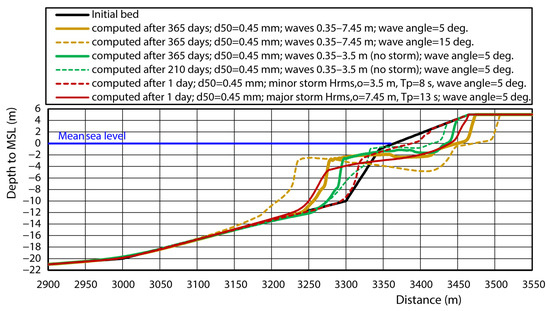
Figure 20. Effect of offshore wave climate and wave angle on beach erosion.

The effect of the offshore wave incidence angle is also quite strong. When this value is increased from 5° to 15°, the longshore current velocity in the surf zone increases substantially, resulting in higher sand transport rates causing substantially more beach erosion (about 700 m³/m after 1 year; almost a factor of 2 higher).

5.4. Effect of Undertow Current, Wave Asymmetry and Wave Runup

Important hydrodynamic processes in the upper surf zone are i) the offshore-directed undertow current due to breaking waves and ii) the asymmetry of the near-bed orbital velocities (higher onshore-directed and lower offshore-directed velocities). The undertow current can be increased or decreased by a linear scaling input parameter (frip in the range of 0.5 to 1.5, default = 1). The wave asymmetry can be described by two methods (input switch): by Isobe-Horikawa 1982 [46] or by Ruessink et al., 2012 [58].

The effects of the undertow current and the wave asymmetry are shown in Figure 21. Variation in the frip input parameter in the range of 0.5 to 1.5 gives a substantially lower (about 40%) and higher (almost a factor of 2) beach erosion after 1 year. A higher undertow current in the surf zone leads to a higher offshore-directed sediment transport in the surf zone (particularly suspended load transport), and thus to more beach erosion. Values of the maximum undertow current for the two wave conditions from the wave input data are given in Table 2. The highest undertow current in the shallow surf zone with breaking waves is 0.75 m/s for frip = 1 and H_rms,o = 7.45 m, which increases to 1.125 m/s for frip = 1.5.

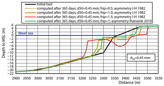
Figure 21. Effect of undertow current and wave asymmetry on long-term beach erosion.

Table 2. Values of undertow velocity and asymmetry of orbital velocity; x = 3358 m is last computation grid point).

Parameter		Hrms,o = 1 m; Tp = 7 s	Hrms,o = 7.45 m; Tp = 13 s
Undertow velocity	frip = 0.5	0.04 m/s at x = 3358 m	0.375 m/s at x = 3358 m
	frip = 1	0.08 m/s at x = 3358 m	0.75 m/s at x = 3358 m
	frip = 1.5	0.12 m/s at x = 3358 m	1.125 m/s at x = 3358 m
Asymmetry of peak orbital velocity	Uon/Uoff	1.33/0.56 m/s at x = 3344 m	2.64/1.17 m/s at x = 3326 m
	I-H 1982 [46]	0.69/0.42 m/s at x = 3358 m	0.6/0.4 m/s at x = 3358 m
	Uon/Uoff	1.62/1.14 m/s at x = 3344 m	2.54/1.6 m/s at x = 3183m
	Ruessink 2012 [58]	0.8/0.62 m/s at x = 3358 m	0.65/0.53 m/s at x = 3358 m

The wave asymmetry has a marked effect on the bed load transport, but not so much on the suspended load transport. Hence, storm-related beach erosion on the time scale of a few days is not significantly affected by the wave asymmetry method [9]. The long-term beach profile changes due to lower daily waves are more affected by the wave asymmetry method, as shown in Figure 21. The method of Isobe-Horikawa 1982 [46] (default method) produces more erosion than the method of Ruessink 2012 [58], mainly because the latter method produces higher peak onshore velocities for low daily waves, resulting in a higher onshore-directed bed load transport in the surf zone, which reduces erosion due to suspended load transport; see values for H_rms,o = 1 m in Table 2.

The effect of wave runup (frunup = 0 to 2) on beach erosion is shown in Figure 22. The input parameter frunup is a multiplication factor with respect to the standard runup (frunup = 1 = default). Frunup = 0.5 only has a minor effect, but frunup = 2 leads to more erosion at the upper beach. Frunup = 0 and 0.1 lead to much less beach erosion.

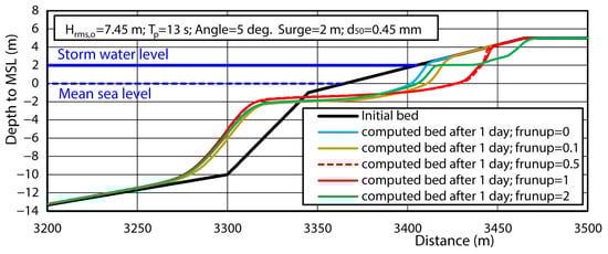
Figure 22. Effect of wave runup for short-term storm case; H_rms,o = 7.45 m (1 day).

5.5. Effect of Sediment Size and Sediment Transport

A novelty is the inclusion of the uniformity coefficient C_u = d₆₀/d₁₀, which is set to 2. This parameter affects the suspended sediment size and thus the settling velocity [32]. More graded sediments have a higher C_u-value, resulting in a smaller suspended sediment size and settling, since the finer particles are winnowed from the bed. This effect is now included in the model, but only has a minor effect [9,32]. The median size d₅₀ has a much stronger effect. Figure 23 shows the computed beach erosion after 1 year (365 days) for four types of sand, d₅₀ = 0.25, 0.45, 0.65 and 1.3 mm, with C_u = 2. The computed beach erosion after 1 year is about 700 m³/m for d₅₀ = 0.25 mm; about 400 m³/m for d₅₀ = 0.45 mm; about 250 m³/m for d₅₀ = 0.65 mm; and about 50 m³/m for d₅₀ = 1.3 mm.

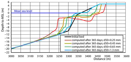
Figure 23. Effect of sand grain size on computed bed profile.

It is clear that the beach erosion reduces substantially when coarser sand is used. The computed beach erosion for sand with d₅₀ = 1.3 mm is more than a factor of 10 smaller than that for sand with d₅₀ = 0.25 mm. The use of fine sand (0.25 mm) is problematic because of excessive erosion after 1 year, requiring immediate maintenance. Overall, the beach is flattened into a submerged platform/berm of deposited sediment at about −2 m below MSL for sand of 0.25 to 0.65 mm. The case with very coarse sand of 1.3 mm shows minor erosion. It is noted that the deposition volume for coarse materials of 1.3 mm landward of x = 3250 m is somewhat larger than the erosion volume because of the supply of sediment from more offshore depths due to wave asymmetry. The bed in the model consists of very coarse sand (1.3 mm) in the whole computational domain, while in practice coarse sand will only be present in the nearshore zone.

The effect of the sand transport rates on the beach erosion is shown in Figure 24.

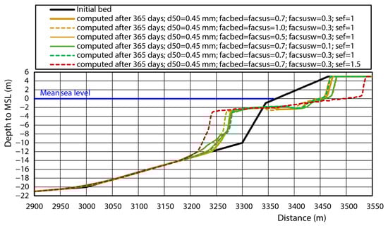
Figure 24. Effect of sediment transport on the beach erosion.

Three modes of sand transport are included in the CROSMOR-model: (i) bed load transport, (ii) offshore-directed current-related suspended load transport and (iii) onshore-directed wave asymmetry-related suspended load transport. These transport rates can be linearly scaled (calibrated) by the following input parameters: facbed, facsus and facsusw (default = 1). Practical experience has shown that the facsusw parameter should be set to a value smaller than 0.3, otherwise too much beach growth is predicted due to onshore transport. A variation in facbed and facsus in the range of 0.5 to 1 shows a limited variation (±10%) in the computed beach erosion after 1 year. Similarly, a variation in the facsusw parameter in the range of 0.1 to 0.3 shows a minor variation (±10%) of the beach erosion.

Finally, the effect of the sef input parameter (range = 1–2; default = 1) is shown. This parameter enhances the bed–shear stress and sediment erosion at steep slopes (dune face). The beach and dune erosion increases substantially (almost factor of 2) for sef = 1.5.

6. Effect of Erosion Reducing Measures

6.1. General

Various alternative methods can be used to reduce beach erosion as much as possible: (1) mild beach slopes, (2) layers of coarse gravel/shingle on top of the sand beach and (3) the construction of a submerged or emerged breakwater in the surf zone at some distance from the shoreline [56]. The effect of mild and steep beach slopes on the beach erosion due to storms has been extensively studied earlier [9,32,59]. Herein, the attention is focused on the effects of a coarse top layer and the construction of a breakwater in the surf zone.

It is noted that the two erosion-reducing options are presented solely in terms of physical performance. For decision-making support, these options should also be studied from a cost–benefit analysis (CBA) perspective. Established CBA methodologies/tools exist, as well as examples already applied to coastal interventions [60,61].

6.2. Effect of Coarse Gravel-Type Top Layer

The placement of a top layer of coarse gravel/shingle (20–40 mm) material on a sandy beach is a promising method to reduce beach erosion, particularly in the case of an artificial land reclamation of sand. This method was used along the beach of Magdalen Island, Saint Lawrence Bay, Canada [62].

The CROSMOR-model has been used to assess to what extent the use of a layer of coarse materials can reduce the beach erosion due to a storm event (H_s,o = 5 m, T_p = 14 s, wave incidence angle θ_o = 10°; file case4ge.inp). The beach profile is a relatively steep profile of a land reclamation of sand with d₅₀ = 0.4 mm. Conservative model settings are used, and the storm duration is set to 3 days (72 h) to promote erosion. The reference case is a beach profile consisting of sand, with d₅₀ = 0.4 mm resulting in an excessive erosion volume of about 380 m³/m after 3 days; see Figure 25. When a coarse top layer is placed along the whole profile, the beach erosion at the upper beach is reduced to about 10 m³/m after 3 days, and slightly more after 10 days of storm. Minor deposition can be observed at the toe of the beach. The bed profile seaward of the −3 m depth line remains stable.

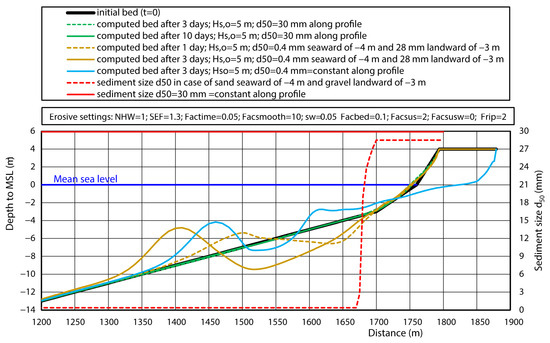
Figure 25. Effect of top layer of coarse materials on beach erosion; major storm, H_s,o = 5 m.

The placement of coarse material along the whole profile is not practical or economical. Observations of gravel transport at gravel/shingle coasts show that coarse materials are, in the long term, always carried onshore due to wave asymmetry effects. Therefore, a more economical solution is the placement of coarse materials in the nearshore zone landward of −3 m depth, while the bed seaward of −3 m depth remains as a sand bed (0.4 mm). This type of composite bed with sand and gravel can be represented by the CROSMOR-model using the multiple fractions method. In all, seven fractions have been used: mostly sand (0.4 mm) seaward of −4 m depth, a transition zone between −4 m and −3 m consisting of both sand and gravel and a coarse gravel layer (28 mm) landward of −3 m depth; see Table 3. It is noted that this is an exploratory computation given the lack of experience with this type of complex composite bed modeling. The computed bed levels are shown in Figure 25. The sediment size is d₅₀ = 0.4 mm for x < 160 m and 29 mm for x > 1700 m. The sediment size increases strongly from 0.4 mm to 28 mm in the transition layer between x = 1650 and 1700 m. The bed profile after a storm with H_s,o = 5 m with a duration of 3 days shows that the upper beach of gravel is rather stable, while the sand bed shows severe erosion and deposition in the form of a breaker bar. The breaker bar at x = 1400 m is rather high, which is caused by the long duration of the storm with a constant maximum wave height (3 days with H_s,o = 5 m), which is not very realistic.

Table 3. Sediment fractions used in CROSMOR-model (file cas4fre.inp; cas4fra.inp).

X-location (m) (bed level)	Fr 1 0.2–0.6 (mm)	Fr 2 0.6–1.8 (mm)	Fr 3 1.8–3.6 (mm)	Fr 4 3.6–7.2 (mm)	Fr 5 7.2–14.4 (mm)	Fr 6 14.4–28.8 (mm)	Fr 7 28.8–57.6 (mm)
0 (−37 m)	0.9	0.02	0.02	0.02	0.02	0.01	0.01
1650 (−4 m)	0.9	0.02	0.02	0.02	0.02	0.01	0.01
1700 (−3 m)	0.02	0.02	0.02	0.02	0.02	0.1	0.8
1760 (0 m)	0.02	0.02	0.02	0.02	0.02	0.1	0.8
1794 (4 m)	0.02	0.02	0.02	0.02	0.02	0.1	0.8
1879 (4 m)	0.02	0.02	0.02	0.02	0.02	0.1	0.8

Figure 26 shows the model results for a minor storm event, with H_s,o = 3 m (T_p = 13 s; wave incidence angle θ_o = 10°; file case4ga.inp). Under these conditions, the coarse materials tend to move onshore (accretive conditions). Therefore, more accretive model settings are used. In the case of a fully sand bed with d₅₀ = 0.4 mm, beach erosion is dominant (about 200 m³/m after 3 days). When a coarse top layer is placed along the whole profile, a swash bar is generated by the onshore movement of coarse materials. The material is eroded from the zone between x = 1550 m and 1690 m. This swash bar is absent when the bed seaward of the −4 m depth consists of sand, and a minor breaker bar is generated at the sand bed.

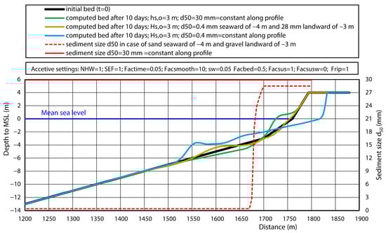
Figure 26. Effect of top layer of coarse materials on beach erosion; minor storm, H_s,o = 3 m.

Overall, it is concluded that the CROSMOR-model produces realistic bed profiles for a composite bed consisting of sand in the deeper water and coarse gravel in the nearshore beach zone. The beach erosion is significantly reduced when the beach is covered with a top layer of coarse materials (20 to 40 mm). More research is required to better understand the model behavior with multiple sediment fractions.

6.3. Effect of Breakwater in the Surf Zone

Another method to reduce beach erosion is the construction of a submerged/emerged breakwater in the surf zone at some distance from the shoreline; see Figure 27.

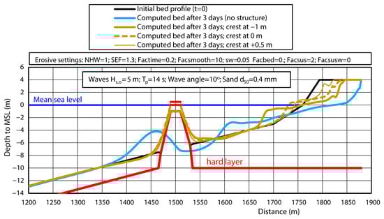
Figure 27. Effect of breakwater on beach erosion; storm, H_s,o = 5 m.

The crest should be designed at −1 m below MSL or higher to be effective. A structure can be represented in the CROSMOR-model as a hard layer. Sand on top of the hard layer can be eroded, but sand under the hard layer cannot be eroded. Sand transport over the exposed hard layer is kept constant, as no sand can be eroded. The deposition of sand on the hard layer can always take place.

Figure 27 shows the computed bed profiles for a storm of H_s,o = 5 m (T_p = 14 s, wave incidence angle θ_o = 10°, storm setup = 1.5 m) with a duration of 3 days. The tidal range is 1.8 m. The bed is sand, with d₅₀ = 0.4 mm. The beach erosion for the case without structure is about 380 m³/m after 3 days, which can be reduced to about 200 m³/m (reduction of 45%) for a breakwater with a crest at −1 m, to about 110 m³/m (reduction of 70%) for a crest at 0 m and to about 65 m³/m (reduction of 85%) for a crest at +0.5 m.

A breakwater with a low crest below −1 m is not very effective. The main reason is that relatively high waves can pass over the crest in conditions with tides and storm setup values of 1 to 2 m [25]. This was also found by Musumeci et al., 2012 [63], for a perched beach with a sill crest at −2.5 m below MSL at a coastal site in Italy. The observed beach retreat at the field site with a sill was of the order of 10 to 15 m after 2 years. Groenewoud et al., 1996 [64], made a scale model (1 to 15) of a sill with a crest at −1.5 m protecting a beach with a slope of 1 to 15 (sand d₅₀ = 0.1 mm). The approach storm wave height was H_s,o = 2 m at a depth of 6 m (on the seaward side of the sill). The beach erosion was reduced by not more than 15%.

Finally, it is noted that the construction of a breakwater in the surf zone is relatively expensive, but an advantage is that the beach can still be used for recreation, which is more problematic if the beach is armored with a coarse top layer.

7. Summary, Discussion and Conclusions

A detailed process-based coastal profile model (CROSMOR) is described, improved and validated for sand and gravel coasts. The new model improvements are (1) an improved more general runup equation based on the available field data; (2) the inclusion of the uniformity coefficient (C_u = d₆₀/d₁₀) of the bed material affecting the settling velocity of the suspended sediment; (3) the inclusion of hard bottom layers, so that the effect of a submerged breakwater on the beach–dune erosion can be assessed; and (4) the determination of adequate model settings for the accretive and erosive conditions of coarse gravel–shingle types of coasts (sediment range of 2 to 40 mm). The improved model has been extensively validated for sand and gravel coasts. The sand validation cases refer to the storm-related erosion of two test dunes constructed and monitored at the Sand Motor site (The Netherlands) in the winter period of 2021–2022 and to a natural sand dune at the beach site De Haan in Belgium. The hindcast simulations were quite good, with high Brier Skill Scores of 0.8 to 0.9. The main calibration parameters of the field validation cases are summarized in Table 4. The bed load transport correction coefficient (facbed) is found to be smaller (0.5) than the default value of 1. The suspended load transport correction coefficient (facsus) is close to the default value of 1. The onshore-directed suspended load transport is negligible (facsusw = 0) for storm events. The SEF parameter (sediment entrainment due to direct wave impact on steep faces) is close to the default value of 2 for storm-related dune erosion. The hindcast simulation for the long-term run over 3 years for the nourishment coastal profile of km 25 at the Petten site (Netherlands) is also reasonable, with a Brier Skill Score of 0.55 for the nearshore zone landward of the bar trough area. This latter area is strongly influenced by 3D effects (erosion due to longshore current), which cannot be represented by the profile model. The facbed parameter has to be set to a low value of 0.2, otherwise too much sand is carried onshore in the long term.

Table 4. Calibration parameters of CROSMOR field validation cases.

Parameters	Sand Dune Erosion Sand Motor (NL)	Sand Dune Erosion De Haan (BE)	Sand Beach Erosion Petten (NL)	Gravel Slapton Sands (UK)	Gravel Chesil Beach (UK)
Waves Hs,o (m	1.4–4.3	1.7–4.8	1.4–5.1	4.7	7.7
Wave period Tp (s)	6–10	4.8–7.3	5–10	9.5	13.9
Wave angle θo (°)	10	5	5	5	5
Grain diameter d50 (mm)	0.3	0.23	0.3	6	40
Uniformity Cu (−)	2	2	2	2	2
Coefficient BLT facbed (−)	0.5	0.5	0.2	0.5	0.3
Coefficient SLT facsus (−)	1.1	1.0	0.6	2	3
Coefficient SLT facsusw (−)	0	0	0	0	0
Coefficient extra sand entrainment dune zone SEF (−)	2	1.5	1.15	2	2
Increased undertow frip (−)	1	1	1	f	3
Bed roughness (m)	0	0	0	0.02	0.08
Brier Skill Score (−)	0.9	0.82	0.55	0.85	0.8

The model has also been extensively tested and validated for a coarse gravel coast. The correction factor (frip) of the undertow velocity has to be increased for a steep gravel coast (frip > 1). The sediment transport formulations of the model can also be used for gravel, although the model tends to underpredict for very coarse gravel. This can be corrected by the facsus parameter being 2 for 6 mm gravel and 3 for 40 mm gravel. Hindcast simulations for the gravel profiles at Chesil beach and Slapton Sands in the UK show significantly high Brier Skill Scores (0.8–0.85).

An extensive series of sensitivity computations have been made to study the key physical parameters (sediment size, wave height, wave incidence angle, wave asymmetry, wave-induced undertow, wave runup), conditions which have a relatively strong effect on the beach erosion processes.

Of course, the wave height and the wave chronology are important parameters. The beach erosion increases strongly for increasing offshore wave height, but the chronology of a major storm is also important, particularly for a new coast (land reclamation or beach nourishment). A major storm hitting the new coastal profile soon after the completion of the construction work causes much more damage than later when the profile has been deformed into a profile with nearshore bars, berms and platforms. The offshore wave incidence angle also has a strong effect on beach erosion because stronger longshore currents are generated for more oblique incoming waves. Similarly, wave asymmetry under shoaling and breaking waves, cross-shore return current (undertow) and wave runup are all key influential parameters which should be varied by changing input parameters to obtain a proper feeling for the variability of these parameters on the computed bed profiles, particularly for long-term runs. A basic parameter is the sediment size, which is fixed for an existing coast but can be changed to some extent for a beach nourishment or a land reclamation site. Beach erosion decreases strongly for coarser sediments. The beach erosion is a factor of 10 smaller for a beach with coarse sand of 1.3 mm compared to a beach with fine sand of 0.25 mm.

Beach erosion at a land reclamation site can be strongly reduced by placing a layer of coarse gravel (20 to 40 mm) on the sand beach. The placement of coarse materials along the whole profile is not practical or economical. Observations of gravel transport at gravel/shingle coasts show that coarse materials are, in the long term, always carried onshore due to wave asymmetry effects. Therefore, the coarse materials should only be placed in the nearshore zone landward of the −3 m depth line, while the bed seaward of the −3 m depth line can remain as a sand bed. This type of composite bed with sand and gravel can be represented by the CROSMOR-model using the multiple fractions method, but at the present stage of research these types of complex computations are still very exploratory due to a lack of experience. More research is required to better understand the behavior of multiple sediment fractions in the nearshore zone. Another method to reduce beach erosion is the construction of a submerged or emerged breakwater in the surf zone at some distance from the shoreline. The crest should be designed at −1 m below MSL or higher to be really effective. A structure can be represented in the CROSMOR-model as a hard layer. The sand on top of the hard layer can be eroded, but the sand under the hard layer cannot be eroded. Sand transport over the exposed hard layer is kept constant, as no sand can be eroded. The deposition of sand on the hard layer can always take place. Example computations show that beach erosion can be significantly reduced by a structure with a relatively high crest level. An advantage of a breakwater structure over the use of a coarse top layer is that the beach can still be used for beach recreation.

Special attention should always be given to model accuracy by using small grid sizes in the nearshore where the cross-shore gradients of wave heights and sediment transport are relatively large. Sensitivity runs should be performed by reducing the grid sizes until the computed bed profiles only show marginal differences. This should also be performed for the (inevitable) bed-smoothing coefficients, which are necessary for obtaining stable bed profiles, particularly for long-term runs over years.

Overall, it is concluded that process-based profile models are quite powerful tools for quick insights on wave heights, cross-shore and longshore currents, sediment transport and beach profile erosion for sand and gravel coasts. This type of model should be available t the desktop of a coastal engineer. The new more generally valid wave runup equation produces more accurate values. The new C_u-coefficient can be used for a bed of non-uniform sand (wide size distribution) to better represent the finer suspended load. The inclusion of hard layers makes it possible to represent submerged breakwaters, but the wave transmission across the breakwater has to be improved (future research). The CROSMOR-model has a simple input file and runs can be made quickly (< 1 h), which makes the model very suitable for quick-scan analysis to obtain a better understanding of the physical processes (nearshore waves, setup, runup, currents) and to study erosion-reducing measures. Output files can be simply imported in Excel for the plotting of results. Run times are very small (1 to 10 min) for short-term runs, but can take hours for long-term runs (years). Finally, it is noted that these types of models perform best in the short term for a system which is out equilibrium (nourishments, structures, etc.). Long-term predictions to find the equilibrium situation including breaker bars remain (too) problematic [15,16,17,18].

References

- Roelvink, J.A.; Broker, I. Cross-shore profile models. Coast. Eng. 1993, 21, 163–191. [Google Scholar] [CrossRef]
- Stive, M.J.F. A model for cross-shore sediment transport. In Proceedings of the 8th ICCE, Taipeh, Taiwan, 1 September 1986; pp. 1550–1554. [Google Scholar]
- Roelvink, J.A.; Meijer, T.; Houwman, K.; Bakker, W.; Spanhoff, R. Field validation and application of a coastal profile model. In Coastal Dynamics; ASCE: Gdansk, Poland, 1995; pp. 818–828. [Google Scholar]
- Steetzel, H. Cross-Shore Transport During Storm Surges. Ph.D. Thesis, Delft University of Technology, Delft, The Netherlands, 1993. [Google Scholar]
- Nairn, R.B.; Southgate, H.N. Deterministic profile modelling of nearshore processes; Part 2, Sediment transport and beach profile development. Coast. Eng. 1993, 19, 57–96. [Google Scholar] [CrossRef]
- Van Rijn, L.C.; Wijnberg, K. One-Dimensional modelling of individual waves and wave-induced currents in the surf zone. Coast. Eng. 1996, 28, 121–145. [Google Scholar] [CrossRef]
- Van Rijn, L.C. The effect of sediment composition on cross-shore bed profiles. In Proceedings of the 26th ICCE, Copenhagen, Denmark, 22–26 June 1998. [Google Scholar]
- Van Rijn, L.C. Prediction of dune erosion due to storms. Coast. Eng. 2009, 56, 441–457. [Google Scholar] [CrossRef]
- Van Rijn, L.C. Crosmor-Applications. 2025. Available online: www.leovanrijn-sediment.com (accessed on 1 September 2025).
- Van Rijn, L.C.; Walstra, D.J.R.; Grasmeijer, B.; Sutherland, J.; Pan, S.; Sierra, J.P. The predictability of cross-shore bed evolution of sandy beaches at the time scale of storms and seasons using process-based profile models. Coast. Eng. 2003, 47, 295–327. [Google Scholar] [CrossRef]
- Kobayashi, N.; Farhadzadeh, A. Cross-Shore Numerical Model CSHORE for Waves, Currents, Sediment Transport and Beach Profile Evolution; Report CACR-08-01; Center for Applied Coastal Research, Ocean Engineering Laboratory; University of Delaware: Newark, DE, USA, 2008. [Google Scholar]
- Roelvink, D.; Reniers, A.; Van Dongeren, A.; Van Thiel de Vries, J.; McCall, R.; Lescinski, J. Modelling storm impacts on beaches, dunes and barrier islands. Coast. Eng. 2009, 56, 1133–1152. [Google Scholar] [CrossRef]
- McCall, R.T.; Masselink, G.; Poate, T.G.; Roelvink, J.A.; Almeida, L.P. Modelling the morphodynamics of gravel beaches during storms with XBeach-G. Coast. Eng. 2015, 103, 52–66. [Google Scholar] [CrossRef]
- Ruessink, B.G.; Kuriyama, Y.; Reniers, A.J.H.M.; Roelvink, J.A.; Walstra, D.J.R. Modeling cross-shore sandbar behavior on the timescale of weeks. J. Geophys. Res. 2007, 112, 1–15. [Google Scholar] [CrossRef]
- Grasmeijer, B.T.; Van Rijn, L.C.; Walstra, D.J. Modeling cross-shore bar behavior on storm and seasonal time scales. In Proceedings of the 28th ICCE, Cardiff, UK, 16–19 September 2002. [Google Scholar]
- Walstra, D.J.; Ruesink, G. Process-based modelling of cyclic bar behaviour on yearly scales. In Proceedings of the Coastal Dynamics 2009: Impacts of Human Activities on Dynamic Coastal Processes, Tokyo, Japan, 7–11 September 2009; p. 54. [Google Scholar] [CrossRef]
- Rafati, Y.; Hsu, T.J.; Elgar, S.; Raubenheimer, B.; Quataert, E.; Van Dongeren, A. Modeling the hydrodynamics and morphodynamics of sand bar migration events. Coast. Eng. 2021, 166, 103885. [Google Scholar] [CrossRef]
- Zhang, J.; Tsai, B.; Rafati, Y.; Hsu, T.J.; Puleo, J.A. Cross-shore hydrodynamics and morphodynamics modeling of an erosive event in the inner surf zone. Coast. Eng. 2025, 196, 104662. [Google Scholar] [CrossRef]
- Vellinga, P. Beach and Dune Erosion During Storm Surges. Ph.D. Thesis, Delft University of Technology, Delft, The Netherlands, 1986. [Google Scholar]
- Deltares. Technical Report Dune Erosion; Report H4357; Delft Hydraulics: Delft, The Netherlands, 2007. (In Dutch) [Google Scholar]
- Dean, R.G. Equilibrium beach profiles: Characteristics and applications. J. Coast. Res. 1991, 7, 53–84. [Google Scholar]
- Larson, M.; Kraus, N.C. SBEACH: Numerical Model for Simulating Storm-Induced Beach Change; Report 1: Empirical Foundation and Model Development; Technical Report CERC-89-9; U.S. Army Engineer Water-Ways Experiment Station: Vicksburg, MS, USA, 1989. [Google Scholar]
- Larson, M.; Kraus, N.C. Mathematical modelling of the fate of beach fill. In Artificial Beach Nourishments: Coastal Engineering; Special Issue; Niemayer, H.D., van Overeem, J., van de Graaff, J., Eds.; Elsevier: Amsterdam, The Netherlands, 1991; Volume 16, pp. 83–114. [Google Scholar]
- Larson, M.; Palalane, J.; Fredriksson, C.; Hanson, H. Simulating cross-shore material exchange at decadal scale. Theory and model component validation. Coast. Eng. 2016, 116, 57–66. [Google Scholar] [CrossRef]
- Marinho, B.; Coelho, C.; Larson, M.; Hanson, H. Cross-shore modelling of multiple nearshore bars at a decadal scale. Coast. Eng. 2020, 159, 103722. [Google Scholar] [CrossRef]
- Romao, F.; Coelho, C.; Lima, M.; Ásmundsson, H.; Myer, E.M. Cross-Shore Modeling Features: Calibration and Impacts of Wave Climate Uncertainties. J. Mar. Sci. Eng. 2024, 12, 760. [Google Scholar] [CrossRef]
- Diez, J.; Uriarte, A.; Canovas, V.; Medina, R. A parametric model for dry beach equilibrium profiles. Coast. Eng. 2017, 127, 134–144. [Google Scholar] [CrossRef]
- Kettler, T.; de Schipper, M.; Luijendijk, A. Simulating decadal cross-shore dynamics at nourished coasts with Crocodile. Coast. Eng. 2024, 190, 104491. [Google Scholar] [CrossRef]
- Kim, J.; Kim, T.; Chang, S.; Kim, J.; Kim, I. Prediction of beach profile changes using spatiotemporal graph neural networks for beach morphological evolution modeling. Ocean Eng. 2025, 340, 122282. [Google Scholar] [CrossRef]
- Ken Muroi, S.; Bertone, E.; Cartwright, N.; Alvarez, F. Machine Learning methods for predicting shoreline change from submerged breakwater simulations. Eng. Appl. Artif. Intell. 2025, 125, 110726. [Google Scholar] [CrossRef]
- Munian, S.; Karakus, O.; Russell, W.; Nelson, G. Topoformer: Integrating Transformers and ConvLSTMs for Coastal Topography Prediction. arXiv 2025, arXiv:2501.06494v1. [Google Scholar]
- Van Rijn, L.C.; Mol, A.; Kroeders, M. Design of artificial beaches at sheltered and exposed sites. J. Environ. Earth Sci. 2025, 7, 588–610. [Google Scholar] [CrossRef]
- Van Rijn, L.C. Unified view of sediment transport by currents and waves, I: Initiation of motion, bed roughness, and bed-load transport. J. Hydraul. Eng. 2007, 133, 649–667. [Google Scholar] [CrossRef]
- Van Rijn, L.C. Unified view of sediment transport by currents and waves, II: Suspended transport. J. Hydraul. Eng. 2007, 133, 668–689. [Google Scholar] [CrossRef]
- Van Rijn, L.C. Unified view of sediment transport by currents and waves, III: Graded Beds. J. Hydraul. Eng. 2007, 133, 761–775. [Google Scholar] [CrossRef]
- Guza, R.T.; Thorton, E.B. Swash oscillations on a natural beach. J. Geophys. Res. 1982, 87, 483–490. [Google Scholar] [CrossRef]
- Douglass, S.L. Estimating extreme values of runup on beaches. Journal of Waterway, Port, Coastal, and Ocean Engineering. Am. Soc. Civ. Eng. 1992, 118, 220–224. [Google Scholar]
- Nielsen, P.; Hanslow, D.J. Wave runup distributions on natural beaches. J. Coast. Res. 1991, 7, 1139–1152. [Google Scholar]
- Stockdon, H.F.; Holman, R.A.; Howd, P.A.; Sallenger, A.H. Empirical parameterization of setup, swash and runup. Coast. Eng. 2006, 53, 73–588. [Google Scholar] [CrossRef]
- Senechal, N.; Coco, G.; Bryan, K.R.; Holman, R.A. Wave runup during extreme storm conditions. J. Geophys. Res. 2011, 116, C07032. [Google Scholar] [CrossRef]
- Mase, H. Random wave runup height on gentle slope. J. Waterw. Port Coast. Ocean Eng. Am. Soc. Civ. Eng. 1989, 115, 649–661. [Google Scholar] [CrossRef]
- Van Gent, M.R.A. Wave runup on dikes with shallow foreshores. J. Waterw. Port Coast. Ocean Eng. 2001, 127, 254–262. [Google Scholar] [CrossRef]
- Hughes, S.A. Estimation of wave runup on smooth, impermeable slopes using the wave momentum flux parameter. Coast. Eng. 2004, 51, 1085–1104. [Google Scholar] [CrossRef]
- Poate, T.G.; McCall, R.T.; Masselink, G. A new parameterisation for runup on gravel beaches. Coast. Eng. 2016, 117, 176–190. [Google Scholar] [CrossRef]
- Dodet, G.; Leckler, F.; Sous, D.; Ardhuin, F.; Filipet, J.F.; Suarez, S. Wave runup over steep rocky cliffs. JGR Ocean. 2018, 123, 7185–7205. [Google Scholar] [CrossRef]
- Isobe, M.; Horikawa, K. Study on water particle velocities of shoaling and breaking waves. Coast. Eng. Jpn. 1982, 25, 109–123. [Google Scholar] [CrossRef]
- Malherbe, B.; Helewaut, M. Design and execution of beach nourishments in Belgium. In Proceedings of the Coastal Zone 93, New Orleans, LA, USA, 19–23 July 1993. [Google Scholar]
- Fordeyn, J.; Malherbe, B. Coastal Defence of Lowlands with Sand: Morpho-Dynamic Concepts of Beach-Dune System Rehabilitation. In Proceedings of the 8th International Conference on Coastal and Port Engineering in Developing Countries, COPEDEC, Madras, India, 20–24 February 2012. [Google Scholar]
- Malherbe, B.; Fordeyn, J. Smart beach and dune nourishments to achieve sustainable coastal protection. In Proceedings of the WODCON XX 2013—World Dredging Congress, Brussels, Belgium, 3–7 June 2013. [Google Scholar]
- Van Wiechen, P.; Rutten, J.; Mieras, R.; Anarde, K.; Wrobel, M.; Tissier, M.; De Vries, S. The real dune/reflex experiment at the sand engine 75–77). In Book of Abstracts Building Coastal Resilience; Special Publication; Strypsteen, G., Roest, B., Bonte, D., Rauwoens, P., Eds.; Flemish Institute for the Sea: Oostende, Belgium, 2022; p. 89. [Google Scholar] [CrossRef]
- Rijkswaterstaat. JARKUS Database. 2025. Available online: www.data/overheid.nl (accessed on 23 August 2025).
- Meyer-Peter, E.; Mueller, R. Formulas for bed load transport. In Proceedings of the IAHR 2nd Meeting, Stockholm, Sweden, 7 June 1948; pp. 41–64. [Google Scholar]
- Chadwick, A.J. Field measurements and numerical model verification of coastal shingle transport, Chapter 27. In Advances in Water Modelling and Measurements; Palmer, M.H., Ed.; BHRA, Fluid Engineering Centre: Bedford, UK, 1989; pp. 381–402. [Google Scholar]
- Nicholls, R.J.; Wright, P. Longshore transport of pebbles: Experimental estimates of K-factor. In Coastal Sediments; ASCE: Seattle, WA, USA, 1991; pp. 920–933. [Google Scholar]
- Deltares/Delft Hydraulics. Scale Effects in Stability of Gravel and Stone Slopes Under Wave Attack in Deltaflume; Report M1983 Part IV; Deltares/Delft Hydraulics: Delft, The Netherlands, 1989. (In Dutch) [Google Scholar]
- López de San Román-Blanco, B.; Coates, T.; Holmes, P.; Chadwick, A.; Bradbury, A.; Baldock, T.; Pedrozo Acuña, A.; Lawrence, J.; Grune, J. Large scale experiments on gravel and mixed beaches. Coast. Eng. 2006, 53, 349–362. [Google Scholar] [CrossRef]
- Buscombe, D.; Williams, J.J.; Masselink, G. Barrier Dynamics Experiments (BARDEX), Experimental Procedure, Technical Information and Data Report; School of Geography, University of Plymouth: Plymouth, UK, 2008. [Google Scholar]
- Ruessink, B.G.; Ramaekers, G.; Van Rijn, L.C. On the parameterization of the free-stream non-linear wave orbital motion in nearshore morphodynamic models. Coast. Eng. 2012, 65, 56–63. [Google Scholar] [CrossRef]
- Van Rijn, L.C. Design and effectiveness of coastal protection structures; case studies and modeling approaches. J. Environ. Earth Sci. 2025, 7, 72–95. [Google Scholar] [CrossRef]
- Pais-Barbosa, J.; Ferreira, A.M.; Lima, M.; Magalhães Filho, L.; Roebeling, P.; Coelho, C. Cost-benefit analysis of artificial nourishments: Discussion of climate change adaptation pathways at Ovar (Aveiro, Portugal). Ocean Coast. Manag. 2023, 244, 106826. [Google Scholar] [CrossRef]
- Lima, M.; Coelho, C. Assessing costs and benefits of coastal structures to mitigate erosion. In Coastal Structures; Goseberg, N., Schlurmann, T., Eds.; Bundesanstalt fur Wasserbau: Karlsruhe, Germany, 2019. [Google Scholar] [CrossRef]
- Van Rijn, L.C. Modelling of Longshore Gravel Transport at Gravel Beach Nourishment Magdalen Island, Saint Lawrence Bay, Canada; Technical Report; LVRS-Consultancy: Blokzijl, The Netherlands, 2025; Available online: www.leovanrijn-sediment.com (accessed on 1 September 2025).
- Musumeci, R.E.; Cavallaro, L.; Foti, E. Performance of perched beach nourishments. In Proceedings of the 33rd International Conference on Coastal Engineering ICCE, Santander, Spain, 1–3 August 2012. [Google Scholar]
- Groenewoud, M.D.; Van de Graaff, J.; Claessen, E.W.M.; Van der Biezen, S.C. Effect of submerged breakwater on profile development. In Proceedings of the 25th ICCE, Orlando, FL, USA, 2 September 1996; pp. 2428–2441. [Google Scholar]
Disclaimer/Publisher’s Note: The statements, opinions and data contained in all publications are solely those of the individual author(s) and contributor(s) and not of MDPI and/or the editor(s). MDPI and/or the editor(s) disclaim responsibility for any injury to people or property resulting from any ideas, methods, instructions or products referred to in the content. |
© 2025 by the authors. Licensee MDPI, Basel, Switzerland. This article is an open access article distributed under the terms and conditions of the Creative Commons Attribution (CC BY) license (https://creativecommons.org/licenses/by/4.0/).