Influence of Bed Variations on Linear Wave Propagation beyond the Mild Slope Condition

Abstract

As water waves travel from deep to shallow waters, they experience increased nonlinearity and decreased dispersion due to the reduced water depth. While the impact of bed slope on wave propagation celerity is documented, it is often overlooked in commonly used depth-integrated wave models. This study uses the WKB approximation and solves higher-order slope-related terms to analyze the influence of varying depth, including the gradient and laplacian of water depth. One result is an extended longwave for linear wave reflection and transmission on a ramp to deeper waters. The main outcome and focus of this work, however, is a new, simple analytical expression for linear dispersion that includes bed variations. The results are applied to two cases: wind-generated water wave propagation in the nearshore, emphasizing corrections to bathymetry inversion methods, and tsunami propagation over the continental slope, highlighting the limitations of neglecting slope on dispersion and the significant role of the Laplacian of water depth.

1. Introduction

As wind-generated water waves travel from the depths of the ocean toward shallower coastal regions, the diminishing depth has significant implications for their propagation. In deep waters, nonlinear effects are usually minimal, and the waves remain unaffected by the seabed, meaning that their propagation is independent of depth. In this regime, dispersive effects dominate, leading to different celerities for different wave frequencies. However, as waves enter intermediate to shallow waters, where they begin to feel the bottom—i.e., where wave propagation is influenced by water depth—nonlinear effects can become significant, and dispersive effects are reduced. In fact, in shallow waters, celerity depends solely on water depth and becomes independent of wave frequency (i.e., there is no dispersion).

For both practical and scientific purposes, water wave propagation models must be computationally efficient. This necessity leads to a key simplification: depth-integrating the governing equations to derive a system of two-dimensional equations [1,2,3,4]. Additionally, it is common practice to assume that the flow is inviscid and irrotational, which is a good approximation except within the thin bottom boundary layer and during wave breaking. The effects of the boundary layer and wave breaking are typically incorporated into the energy equation [5,6,7]. Further simplifications involve time-averaging the governing equations to bypass resolving the wave phase, allowing a focus on wave statistics over large spatial domains [8].

Regarding phase-resolving equations, which is the focus here, although depth-integrated and irrotational, they must still effectively capture nonlinear, dispersive, and bed slope effects. These models can be broadly categorized into two largely complementary families: those derived from Airy theory and those based on the Shallow-Water Equations (SWEs).

Airy theory is fully dispersive, i.e., valid for arbitrary depths, but it is applicable only to small-amplitude waves [2,9]. Further, it is limited to flat beds. Despite its simplicity, Airy theory provides linear equations that yield useful approximate expressions for velocity profiles, pressure fields, and other wave characteristics. One fundamental result from Airy theory is the dispersion relationship, which relates the wave angular frequency, $\omega =2\pi /T$ ($T=$ wave period), the wavenumber, $k=2\pi /L$ ($L=$ wavelength), and the water depth, h. This relationship, valid in principle for flat beds, is given by [10] (Burnside)

$${\omega }^2=gktanhkh,$$

(1)

where g is the gravitational acceleration. Because of the asymptotic behavior of the hyperbolic tangent, it is commonly considered that $kh\gtrsim \pi$ indicates deep water conditions (where ${\omega }^2=gk$), while $kh\lesssim \pi /10$ indicates shallow waters (where ${\omega }^2=g{k}^{2}h$) [2].

There are two main extensions of the Airy linear theory. The first is Stokes theory [1,11], which introduces a perturbative approach based on wave amplitude to account for nonlinear effects to some extent. While Stokes theory has limitations in shallow waters, it is valuable for applications such as the harmonic decomposition of waves [1]. The second extension involves the Mild-Slope Equations (MSEs) [12,13] and related variants, including the “Modified” and “Complementary” MSEs, e.g., [14,15,16,17]. This family of equations is particularly useful for addressing bed-related phenomena such as wave shoaling, refraction, and diffraction. Given that the MSEs implicitly account for two characteristic lengths—namely, the wavelength and the length scale over which the bed bathymetry changes—the WKB (Wentzel–Kramers–Brillouin) perturbative method is particularly well suited for their derivation [1,18]. Notably, although the MSEs account for bed slope effects, the dispersion Equation (1) remains unchanged. This is because, at the perturbative order considered, the bed can be considered locally flat with respect to dispersion.

On the other hand, the SWEs can handle arbitrary nonlinearity (large-amplitude waves) but only in shallow waters, where the water depth is small compared to the wavelength [19]. Starting from the SWEs and using perturbative techniques, Boussinesq-type equations (BTEs) are derived to incorporate dispersive effects, extending the range of applicability to deeper waters [20,21,22,23,24]. The ability of the BTEs to manage dispersive conditions is typically assessed by comparing the performance of the linearized BTEs against the linear Airy theory, specifically in terms of wave celerity and shoaling behavior [24,25].

The above models do not fully capture the influence of bed slope on wave dispersion, particularly in fully dispersive conditions. This work addresses this gap by introducing a new formulation that incorporates bed slope effects into the dispersion Equation (1). In order to achieve this, we apply the WKB approximation to a sufficient order, enabling us to accurately capture the effects of bed slope on the dispersion. Actually, the limitations of the Burnside equation are already well documented. Broadly speaking, if $\sigma$ represents the slope, its influence can be neglected only when [18]

$${\displaystyle \frac{\sigma }{kh}},$$

is small. Importantly, it is not just $\sigma$ that must be small, but rather $\sigma /k$ must be small compared to h, where $\sigma /k=2\pi \sigma L$ is a measure of the depth change over a wavelength. Thus, the same slope $\sigma$ can be considered mild or steep depending on $kh$, with slopes appearing milder in deep waters (large $kh$) and steeper in shallow waters (small $kh$). For values of $kh$ ranging from approximately $0.46$ to $0.86$, Booij [26] found that the mild slope hypothesis holds when $\sigma \lesssim 1/3$ (expressed in terms of ${\omega }^{2}h/g$ instead of $kh$ in the original work). Therefore, the mild slope condition can be more precisely stated as

$${\displaystyle \frac{\sigma }{kh}}\lesssim 0.38\left\{={\displaystyle \frac{1/3}{0.86}}\right\}.$$

(2)

For very shallow waters and a sloped plane bed, the problem has already been addressed by Ehrenmark [27] (see also [28]). The expression by Ehrenmark [27] reads

$${\omega }^2=gktanh\left({\displaystyle \frac{arctan\sigma }{\sigma }}kh\right),$$

through an asymptotic analysis. Since the above holds only for very shallow waters, the hyperbolic tangent tends to the identity, and

$$k={\displaystyle \frac{\omega }{\sqrt{gh}}}\sqrt{{\displaystyle \frac{\sigma }{arctan\sigma }}}=k_0\left(1+{\displaystyle \frac{{\sigma }^2}{6}}+\mathcal{O}\left({\sigma }^4\right)\right),$$

(3)

where $k_0=\omega /\sqrt{gh}$ is the Burnside solution for shallow waters. According to Equation (3), $k⩾k_0$, so the celerity $c=\omega /k$ is reduced by the slope.

The previous approach is valid only for the asymptotic case of very shallow waters. For the fully dispersive regime, Ge et al. [29] recently presented a dispersion relationship that incorporates bed slope effects, but it is limited to the specific case of sinusoidal bathymetry. In contrast, we derive a more general expression that is fully dispersive and applicable to arbitrary bathymetry. We employ a WKB approach following [1,18] but extend the analysis to higher-order terms. The resulting equation bears a striking resemblance to that proposed by Ge et al. [29], with the critical difference of an opposite sign—a distinction that is highly significant. We then apply the proposed dispersion equation to several important cases to demonstrate the impact of accounting for (or neglecting) bed slope variations in the dispersion relationship.

2. Governing Equations

Throughout the work, $\mathbf{x}=\left(x,y\right)$ will refer to the horizontal coordinates, and z to the vertical one, with $z=0$ at the mean sea water level, $z=\eta$ at the free surface, and $z=-h$ at the bottom (Figure 1 for the one-dimensional case). We use the notation usually employed in water-wave textbooks as, e.g., those by Dean and Dalrymple [2] or Svendsen [3]. Also, as usual in depth-integrated models and many other wave propagation models, the flow is considered inviscid and irrotational [1,2,3,18], and the potential of the velocity is denoted with $\mathsf{\Phi }$. In assuming, hereinafter, a rigid bed, the linearized equations for $\mathsf{\Phi }$ are [18]

$$\begin{array}{ccc}\hfill {\nabla }^2\mathsf{\Phi }+{\displaystyle \frac{{\partial }^2\mathsf{\Phi }}{\partial z^2}}& =0,\hspace{1em}\hspace{1em}\hspace{1em}\hfill & \hfill -h⩽z⩽0,\end{array}$$

(4)

$$\begin{array}{ccc}\hfill \nabla \mathsf{\Phi }·\nabla h+{\displaystyle \frac{\partial \mathsf{\Phi }}{\partial z}}& =0,\hspace{1em}\hspace{1em}\hspace{1em}\hspace{1em} \hfill & \hfill z=-h,\end{array}$$

(5)

$$\begin{array}{ccc}\hfill {\displaystyle \frac{{\partial }^2\mathsf{\Phi }}{\partial t^2}}+g{\displaystyle \frac{\partial \mathsf{\Phi }}{\partial z}}& =0\hspace{1em}\hspace{1em}\hspace{1em}\hspace{1em}\hspace{1em}\hfill & \hfill z=0,\end{array}$$

(6)

where ∇ stands for the horizontal gradient $\left(\partial /\partial x,\partial /\partial y\right)$.

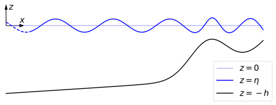
Figure 1. Coordinates x and z (one-dimensional case), and elevations of the mean sea level ($z=0$), free surface ($z=\eta$), and bed ($z=-h$).

Equations (4)–(6) are, respectively, the mass conservation, the kinematic boundary condition at the bottom, and a combination of the kinematic and the dynamic boundary conditions at the free surface. The Bernoulli equation, as well as the kinematic and dynamic boundary conditions at the free surface, is avoided so that the equations are expressed exclusively using the potential $\mathsf{\Phi }$ [3,18]. The linearized kinematic and dynamic boundary conditions at the free surface are, for future use,

$$\begin{array}{ccc}\hfill {\displaystyle \frac{\partial \eta }{\partial t}}-{\displaystyle \frac{\partial \mathsf{\Phi }}{\partial z}}& =0\hspace{1em}\hspace{1em}\hfill & \hfill z=0,\end{array}$$

(7)

$$\begin{array}{ccc}\hfill {\displaystyle \frac{\partial \mathsf{\Phi }}{\partial t}}+g\eta & =0\hspace{1em}\hspace{1em} \hfill & \hfill z=0.\end{array}$$

(8)

The depth-integrated continuity and momentum equations are, e.g., [18],

$$\begin{array}{cc}\hfill \nabla ·{\int }_{-h}^0\nabla \mathsf{\Phi }+{\displaystyle \frac{\partial \eta }{\partial t}}& =0,\hfill \end{array}$$

(9)

$$\begin{array}{cc}\hfill g\nabla \eta +\nabla {\displaystyle \frac{\partial {\mathsf{\Phi }}_{z=0}}{\partial t}}& =0,\hfill \end{array}$$

(10)

and the depth-integrated and time-averaged energy equation is

$$⟨\nabla ·{\int }_{-h}^0{\displaystyle \frac{\partial \mathsf{\Phi }}{\partial t}}\nabla \mathsf{\Phi }dz⟩=0,$$

(11)

where $⟨·⟩$ stands for the time average (i.e., over one wave period anticipating the time-harmonic flow conditions).

2.1. Equations for Time-Harmonic Free-Surface Flows

Assuming a time-harmonic solution, we consider

$$\begin{array}{cc}\hfill \mathsf{\Phi }& ={\mathsf{\Phi }}_{1}exp\left(-i\omega t\right)+complex conjugate,\hfill \end{array}$$

(12)

$$\begin{array}{cc}\hfill \eta & ={\eta }_{1}exp\left(-i\omega t\right)+complex conjugate,\hfill \end{array}$$

(13)

with $\omega$ as the wave angular frequency; ${\mathsf{\Phi }}_1$ and ${\eta }_1$, two complex valued functions of $\mathbf{x}$ and z; and $i=\sqrt{-1}$, the imaginary unit hereinafter. From free-surface boundary condition (8), it is

$${\eta }_1={\displaystyle \frac{i\omega }{g}}{\mathsf{\Phi }}_{1,z=0},$$

(14)

so that ${\eta }_1$ is known if ${\mathsf{\Phi }}_1$, which is the focus herein, is resolved.

As any complex variable, the time-independent ${\mathsf{\Phi }}_1\left(\mathbf{x},z\right)$ can be expressed in its polar form as

$${\mathsf{\Phi }}_1=A\left(\mathbf{x},z\right)exp\left(i\theta \left(\mathbf{x},z\right)\right),$$

(15)

with A and $\theta$ as two real functions (the amplitude and the phase, respectively). Introducing the above Equations (12) and (15) into Equations (4)–(6), we obtain a set of equations with the following real part:

$$\begin{array}{ccc}\hfill {\nabla }^{2}A-A{k}^2+{\displaystyle \frac{{\partial }^{2}A}{\partial z^2}}-A{\displaystyle \frac{\partial \theta }{\partial z}}{\displaystyle \frac{\partial \theta }{\partial z}}& =0,\hspace{1em}\hspace{1em}\hfill & \hfill -h⩽z⩽0,\end{array}$$

(16)

$$\begin{array}{ccc}\hfill \nabla A·\nabla h+{\displaystyle \frac{\partial A}{\partial z}}& =0,\hspace{1em}\hspace{1em}\hspace{1em}\hspace{1em}\hspace{1em}\hspace{1em}\hspace{1em} \hfill & \hfill z=-h,\end{array}$$

(17)

$$\begin{array}{ccc}\hfill -{\omega }^{2}A+g{\displaystyle \frac{\partial A}{\partial z}}& =0,\hspace{1em}\hspace{1em}\hspace{1em}\hspace{1em}\hspace{1em}\hspace{1em} \hfill & \hfill z=0,\end{array}$$

(18)

with $k^2=\nabla \theta ·\nabla \theta$. The imaginary part is

$$\begin{array}{ccc}\hfill 2\nabla A·\nabla \theta +A{\nabla }^2\theta +2{\displaystyle \frac{\partial A}{\partial z}}{\displaystyle \frac{\partial \theta }{\partial z}}+A{\displaystyle \frac{{\partial }^2\theta }{\partial z^2}}& =0,\hspace{1em}\hspace{1em}\hspace{1em}\hspace{1em}\hspace{1em}\hfill & \hfill -h⩽z⩽0,\end{array}$$

(19)

$$\begin{array}{ccc}\hfill A\nabla \theta ·\nabla h+A{\displaystyle \frac{\partial \theta }{\partial z}}& =0,\hspace{1em}\hspace{1em}\hspace{1em}\hspace{1em}\hspace{1em}\hspace{1em}\hspace{1em}\hspace{1em}\hspace{1em}\hspace{1em}\hspace{1em}\hspace{1em}\hfill & \hfill z=-h,\end{array}$$

(20)

$$\begin{array}{ccc}\hfill gA{\displaystyle \frac{\partial \theta }{\partial z}}& =0,\hspace{1em}\hspace{1em}\hspace{1em}\hspace{1em}\hspace{1em}\hspace{1em}\hspace{1em}\hspace{1em}\hspace{1em}\hspace{1em}\hspace{1em}\hspace{1em} \hfill & \hfill z=0.\end{array}$$

(21)

Similarly, in recalling Equation (14), the depth-integrated continuity and energy Equations (9) and (11) read

$$\begin{array}{cc}\hfill \nabla ·{\int }_{-h}^0\left(\nabla A+iA\nabla \theta \right)exp\left(i\theta \right)dz+{\displaystyle \frac{{\omega }^2}{g}}{A}_{z=0}exp\left(i{\theta }_{z=0}\right)& =0,\hfill \end{array}$$

(22)

$$\begin{array}{cc}\hfill \nabla ·{\int }_{-h}^0{A}^2\nabla \theta dz& =0,\hfill \end{array}$$

(23)

The momentum Equation (10) is automatically satisfied in this time-harmonic flow case. In recalling Equations (12) and (13), Equation (10) becomes

$$g\nabla {\eta }_1-i\omega \nabla {\mathsf{\Phi }}_{1,z=0}=0,$$

which is automatically satisfied if, as stated in Equation (14), ${\eta }_1=i{g}^{-1}\omega {\mathsf{\Phi }}_{1,z=0}$.

2.2. The Imaginary Part: Vertical Profile of the Phase

In multiplying by A, Equation (19) is

$$\nabla ·\left(A^2\nabla \theta \right)+{\displaystyle \frac{\partial }{\partial z}}\left(A^2{\displaystyle \frac{\partial \theta }{\partial z}}\right)=0,$$

(24)

so that, by integrating in z from $-h$ to z and using bottom boundary condition (20), we obtain

$${\displaystyle \frac{\partial \theta }{\partial z}}=-{\displaystyle \frac{1}{A^2}}\nabla ·{\int }_{-h}^z{A}^2\nabla \theta dz.$$

(25)

Taking into account the free surface boundary condition (21), the above reduces to (energy) Equation (23) for $z=0$. Equation (25) provides insight into the vertical variation in the phase $\theta$. In the derivation of the Mild-Slope Equation and relatives, the phase is typically assumed to be uniform with respect to the vertical coordinate, i.e., $\partial \theta /\partial z=0$. Solving the (non-uniform) vertical profile to a higher-order accuracy will, however, be necessary to obtain the modified dispersion relationship.

3. The WKB Approximation

Equations in Section 2.1, which do not require any condition on the bottom slope being small, do not have analytical solutions other than trivial solutions. To obtain analytical non-trivial solutions that allow us to understand some relevant aspects of wave propagation (wave celerity, wave shoaling, ...), the bed is usually considered to vary slowly to obtain MSEs and relatives. In this Section 3, we introduce the WKB approximation, the same method used to obtain MSEs, which allows us to rigorously apply this assumption.

Following the usual WKB approximation in water wave propagation problems [18,30], with $\chi$ as a characteristic small value of the bed slope, the slow spatial coordinates ${\mathbf{x}}_{★}=\chi \mathbf{x}$ are introduced. The space derivatives relative to this variable are ${\nabla }_{★}={\chi }^{-1}\nabla$, and consequently,

$${\nabla }_{★}h={\chi }^{-1}\nabla h={\chi }^{-1}\mathrm{𝒪}\left(\chi \right)=\mathrm{𝒪}\left(1\right),$$

i.e., ${\mathbf{x}}_{★}$ allows for the depth variations for that coordinate to be order one. Further, A and $\theta$ are expanded in WKB as (see Dingemans [30], pp. 60–63, for a detailed rationale behind these equations)

$$A=A_0+{\chi }^2{A}_1+\mathrm{𝒪}\left({\chi }^4\right),\theta ={\chi }^{-1}\left({\theta }_0+{\chi }^2{\theta }_1+\mathrm{𝒪}\left({\chi }^4\right)\right),$$

(26)

assuming that $A_i$ and ${\theta }_i$ are slow variables, so that their derivatives ${\nabla }_{★}$ and ${\nabla }_{★}^2$ are order one. From the above expansions, we obtain, e.g.,

$$\nabla A=\chi {\nabla }_{★}{A}_0+{\chi }^3{\nabla }_{★}^2{A}_1+\mathrm{𝒪}\left({\chi }^5\right),{\nabla }^{2}A={\chi }^2{\nabla }_{★}^2{A}_0+\mathrm{𝒪}\left({\chi }^4\right),$$

and

$$\nabla \theta ={\nabla }_{★}{\theta }_0+{\chi }^2{\nabla }_{★}{\theta }_1+\mathrm{𝒪}\left({\chi }^4\right).$$

From the last equation, $\mathbf{k}=\nabla \theta$ and ${\mathbf{k}}_{\mathbf{0}}={\nabla }_{★}{\theta }_0$ are the wavenumber vector and its leading order approximation, respectively, with $\mathbf{k}={\mathbf{k}}_{\mathbf{0}}+\mathrm{𝒪}\left({\chi }^2\right)$, and further,

$$\begin{array}{c}k=\sqrt{\nabla \theta ·\nabla \theta }=\sqrt{{\nabla }_{★}{\theta }_0·{\nabla }_{★}{\theta }_0+2{\chi }^2{\nabla }_{★}{\theta }_0·{\nabla }_{★}{\theta }_1+\mathrm{𝒪}\left({\chi }^4\right)}\hfill \\ \hfill \hspace{1em}\hspace{1em}\hspace{1em}\hspace{1em}\hspace{1em}\hspace{1em}\hspace{1em}\hspace{1em}\hspace{1em}\hspace{1em}\hspace{1em}\hspace{1em}\hspace{1em}\hspace{1em}=\sqrt{{\nabla }_{★}{\theta }_0·{\nabla }_{★}{\theta }_0}+{\chi }^2{\displaystyle \frac{{\nabla }_{★}{\theta }_0·{\nabla }_{★}{\theta }_1}{\sqrt{{\nabla }_{★}{\theta }_0·{\nabla }_{★}{\theta }_0}}}+\mathrm{𝒪}\left({\chi }^4\right),\end{array}$$

i.e.,

$$k=k_0+{\chi }^2{k}_1+\mathrm{𝒪}\left({\chi }^4\right),$$

(27)

where $k_0^2={\nabla }_{★}{\theta }_0·{\nabla }_{★}{\theta }_0$ and $k_1=k_0^{-1}{\nabla }_{★}{\theta }_0·{\nabla }_{★}{\theta }_1$. The main goal of this work is, actually, to obtain the expressions for $k_0$ and $k_1$, and therefore the (linear) dispersion relationship including the influence of the bed variations.

For future use, it is also of interest that, from Equation (25),

$${\displaystyle \frac{\partial \theta }{\partial z}}=-{\displaystyle \frac{\chi }{A_0^2}}{\nabla }_{★}·{\int }_{-h}^z{A}_0^2{\nabla }_{★}{\theta }_{0}dz+\mathrm{𝒪}\left({\chi }^3\right)=\mathrm{𝒪}\left({\chi }^1\right),$$

(28)

so that, in recalling the expansions in Equation (26),

$${\displaystyle \frac{\partial {\theta }_0}{\partial z}}=\left(\chi +\mathrm{𝒪}\left({\chi }^2\right)\right){\displaystyle \frac{\partial \theta }{\partial z}}=\mathrm{𝒪}\left({\chi }^2\right),$$

and therefore,

$${\displaystyle \frac{\partial {\mathbf{k}}_{\mathbf{0}}}{\partial z}}={\displaystyle \frac{\partial }{\partial z}}{\nabla }_{★}{\theta }_0={\nabla }_{★}{\displaystyle \frac{\partial {\theta }_0}{\partial z}}=\mathrm{𝒪}\left({\chi }^2\right).$$

(29)

In order to obtain Equation (28), it has been considered, e.g., that

$${\displaystyle \frac{1}{A^2}}={\displaystyle \frac{1}{A_0^2+2{\chi }^2{A}_0{A}_1+\mathrm{𝒪}\left({\chi }^4\right)}}={\displaystyle \frac{1}{A_0^2}}+\mathrm{𝒪}\left({\chi }^2\right).$$

These kinds of manipulations will often be carried out without being explicitly shown.

4. The Leading-Order Solution

By introducing Expansion (26) into Equations (16)–(18) and noting $\partial \theta /\partial z=\mathrm{𝒪}\left({\chi }^1\right)$ from Equation (28), we obtain, to the leading order,

$$\begin{array}{ccc}\hfill -A_0{k}_0^2+{\displaystyle \frac{{\partial }^2{A}_0}{\partial z^2}}& =0,\hspace{1em}\hspace{1em}\hspace{1em}\hspace{1em}\hfill & \hfill -h⩽z⩽0,\end{array}$$

(30)

$$\begin{array}{ccc}\hfill {\displaystyle \frac{\partial A_0}{\partial z}}& =0,\hspace{1em}\hspace{1em}\hspace{1em}\hspace{1em}\hspace{1em}\hspace{1em}\hspace{1em}\hspace{1em} \hfill & \hfill z=-h,\end{array}$$

(31)

$$\begin{array}{ccc}\hfill -{\omega }^2{A}_0+g{\displaystyle \frac{\partial A_0}{\partial z}}& =0,\hspace{1em}\hspace{1em}\hspace{1em}\hspace{1em}\hspace{1em}\hspace{1em}\hfill & \hfill z=0.\end{array}$$

(32)

4.1. Solution for the Equations

The solution of the above equations, and all the results in this Section 4.1, are well known and given here without detailed explanations [3]. The amplitude $A_0$ is

$$A_0=K_{c0}cosh{q}_0,\left[q_0=k_0\left(z+h\right)\right].$$

(33)

From the free surface condition (32), we obtain

$${\omega }^2=g{k}_{0}tanh{\mu }_0,$$

(34)

which is the leading-order Burnside [10] dispersion relationship. Equations (33) and (34), with constant $K_{c0}$, constitute the Airy solution for water-wave propagation over flat beds [2]. Many interesting phenomena can already be understood from these two equations (deep and shallow water conditions, good approximations of the velocity profile and the pressure field, standing waves, ...).

Even within this leading-order solution, the variations in $K_{c0}$, which is a representation of the wave height, can be estimated due to the water depth changes. From Equation (23), the leading order is

$$\nabla ·\left(K_{c0}^2\left(sinh2{\mu }_0+2{\mu }_0\right){\mathbf{s}}_{\mathbf{0}}\right)=0,\left[{\mu }_0=k_{0}h\right],$$

(35)

where ${\mathbf{s}}_{\mathbf{0}}={\mathbf{k}}_{\mathbf{0}}/k_0$ is the unit vector in the direction of the wave propagation. Expression (35) relates $K_{c0}$ with the water depth, embedded in ${\mu }_0$. It is a fundamental equation in the MSE family.

From Equation (15), ${\mathsf{\Phi }}_1=K_{c0}cosh{q}_{0}exp\left(i\theta \right)$, and from Equation (14),

$${\eta }_1={\displaystyle \frac{i\omega }{g}}{\mathsf{\Phi }}_{1,z=0}={\displaystyle \frac{i\omega }{g}}{K}_{c0}cosh{\mu }_{0}exp\left(i{\theta }_{z=0}\right),$$

or

$${\eta }_1={\displaystyle \frac{i{H}_0}{4}}exp\left(i{\theta }_{z=0}\right),\mathrm{with}{H}_0={\displaystyle \frac{4\omega }{g}}{K}_{c0}cosh{\mu }_0,$$

which is the wave height. In using the wave height, energy Equation (35) is

$$\nabla ·\left(H_0^2{\mathbf{c}}_{\mathbf{g}\mathbf{0}}\right)=0,\mathrm{with}{\mathbf{c}}_{\mathbf{g}\mathbf{0}}={\displaystyle \frac{\partial \omega }{\partial k_0}}{\mathbf{s}}_{\mathbf{0}},$$

which is the group celerity vector. The latter equation has been widely used to understand the shoaling in terms of the wave height as it approaches the shore, and Green’s law is a particular case for shallow waters [2]. Introducing a drag term on the right-hand side has been used to understand the wave attenuation associated with bottom friction [7].

4.2. Spatial Derivatives

To obtain higher-order approximations of the solution in the following Section 5 and Section 6, the gradient and the Laplacian of the main functions obtained in the leading-order solution will be required. For any function f of h, it is

$$\nabla f={\displaystyle \frac{df}{dh}}\nabla h,{\nabla }^{2}f={\displaystyle \frac{df}{dh}}{\nabla }^{2}h+{\displaystyle \frac{d^{2}f}{d{h}^2}}{|\nabla h|}^2,$$

and therefore, $df/dh$ and $d^{2}f/d{h}^2$ suffice to obtain $\nabla f$ and ${\nabla }^{2}f$ as functions of $\nabla h$ and ${\nabla }^{2}h$. Following Schäffer and Madsen [31], we define

$${\alpha }_f=-{\displaystyle \frac{h}{f}}{\displaystyle \frac{df}{dh}},{\beta }_f=-{\displaystyle \frac{h^2}{f}}{\displaystyle \frac{d^{2}f}{d{h}^2}},$$

which are dimensionless, by construction, and it turns out that for the functions we are interested in, they depend solely on ${\mu }_0$. The gradient and Laplacian can be expressed as

$$\nabla f=-{\alpha }_f{\displaystyle \frac{f}{h}}\nabla h,{\nabla }^{2}f=-{\alpha }_f{\displaystyle \frac{f}{h}}{\nabla }^{2}h-{\beta }_f{\displaystyle \frac{f}{h^2}}{|\nabla h|}^2.$$

As shown in Appendix A,

$$\begin{array}{cc}\hfill {\alpha }_{k_0}={\displaystyle \frac{G_0}{1+G_0}},\hspace{1em}\hspace{1em}\hspace{1em}& \hfill G_0={\displaystyle \frac{2{\mu }_0}{sinh2{\mu }_0}},\end{array}$$

(36)

$$\begin{array}{cc}\hfill {\alpha }_{K_{c0}}={\displaystyle \frac{G_0{M}_0}{2{\left(1+G_0\right)}^2}},\hspace{1em}\hspace{1em}\hspace{1em}& \hfill M_0=cosh2{\mu }_0+1.\end{array}$$

(37)

Other functions, such as ${\alpha }_{{\mu }_0}$, ${\beta }_{k_0}$, and ${\beta }_{K_{c0}}$, are also included in Appendix A. In addition, as $q_0=k_0\left(z+h\right)$, we have

$${\displaystyle \frac{d{q}_0}{dh}}={\displaystyle \frac{d{k}_0}{dh}}\left(z+h\right)+k_0={\displaystyle \frac{d{k}_0}{dh}}{\displaystyle \frac{q_0}{k_0}}+k_0={\displaystyle \frac{-{\alpha }_{k_0}{q}_0+{\mu }_0}{h}},$$

(38)

and after manipulation,

$$\begin{array}{cc}\hfill {\displaystyle \frac{\partial A_0}{\partial h}}& ={\displaystyle \frac{K_{c0}}{h}}\left({\delta }_{c0}cosh{q}_0+\left({\delta }_{s1}{q}_0+{\delta }_{s0}\right)sinh{q}_0\right),\hfill \end{array}$$

(39)

$$\begin{array}{cc}\hfill {\displaystyle \frac{{\partial }^2{A}_0}{\partial h^2}}& ={\displaystyle \frac{K_{c0}}{h^2}}\left(\left({ϵ}_{c2}{q}_0^2+{ϵ}_{c1}{q}_0+{ϵ}_{c0}\right)cosh{q}_0+\left({ϵ}_{s1}{q}_0+{ϵ}_{s0}\right)sinh{q}_0\right),\hfill \end{array}$$

(40)

where the functions $\delta$ and $ϵ$ are shown in Table 1.

Table 1. Expressions for $\delta$ and $ϵ$—see Appendix A for $\alpha$ and $\beta$.

	${\delta }_{s1}=-{\alpha }_{k_0}$
${\delta }_{c0}=-{\alpha }_{K_{c0}}$	${\delta }_{s0}={\mu }_0$
${ϵ}_{c2}={\alpha }_{k_0}^2$
${ϵ}_{c1}=-2\mu {\alpha }_{k_0}$	${ϵ}_{s1}=2{\alpha }_{K_{c0}}{\alpha }_{k_0}-{\beta }_{k_0}$
${ϵ}_{c0}={\mu }_0^2-{\beta }_{K_{c0}}$	${ϵ}_{s0}=-2{\mu }_0\left({\alpha }_{K_{c0}}+{\alpha }_{k_0}\right)$

5. Solution to $\mathbf{𝒪}\mathbf{\left(}{\mathit{\chi }}^{\mathbf{1}}\mathbf{\right)}$

Section 5 presents results for $\partial \theta /\partial z$ based on the leading-order solution, which, as shown in Equation (28), is $\mathrm{𝒪}\left({\chi }^1\right)$. The implications of this solution on the classical problem of the wave reflection over a ramp are hinted at.

5.1. The Vertical Profile of the Phase

In recalling the expansions and introducing the solution into Equation (25),

$${\displaystyle \frac{\partial {\theta }_0}{\partial z}}=-{\displaystyle \frac{{\chi }^2}{K_{c0}^2{cosh}^2{q}_0}}{\nabla }_{★}·{\int }_{-h}^z{K}_{c0}^2{cosh}^2{q}_0{\mathbf{k}}_{\mathbf{0}}dz+\mathrm{𝒪}\left({\chi }^4\right).$$

(41)

In taking into account that ${\mathbf{k}}_{\mathbf{0}}$ varies slowly in z—see Equation (29)—the above can be integrated to obtain $\partial {\theta }_0/\partial z$ and, further, to obtain

$${\theta }_0={\theta }_{0b}+{\displaystyle \frac{{\chi }^2{q}_0}{2{\mu }_0}}\left(2{\alpha }_{K_{c0}}tanh{q}_0+{\alpha }_{k_0}{q}_0-2{\mu }_0\right){\nabla }_{★}h·{\mathbf{s}}_{\mathbf{0}}+\mathrm{𝒪}\left({\chi }^4\right),$$

(42)

with ${\mathbf{s}}_{\mathbf{0}}$ being the above-mentioned unit vector in the direction of the wave propagation, and ${\theta }_{0b}$ as a function of $\mathbf{x}$ only—not of z. In recalling that $\theta ={\chi }^{-1}{\theta }_0+\cdots$

$$\theta ={\theta }_b+{\displaystyle \frac{q_0}{2{\mu }_0}}\left(2{\alpha }_{K_{c0}}tanh{q}_0+{\alpha }_{k_0}{q}_0-2{\mu }_0\right)\nabla h·{\mathbf{s}}_{\mathbf{0}}={\theta }_b+\mathrm{𝒪}\left(\chi \right),$$

(43)

with ${\theta }_b={\chi }^{-1}{\theta }_{0b}$.

5.2. Transmission and Reflections on a Ramp

The above results, particularly the vertical profile obtained in Equation (43) for the phase, which has not been described in the literature to the author’s knowledge, allow us here to extend the longwave theory of wave transmission and reflection on a ramp, e.g., ref. [1] to include the dispersion effects. This section is not required for the rest of the work and can be skipped if the reader’s interest is solely in the dispersion relationship including the bed slope influence. Moreover, it is not the author’s intention to thoroughly analyze all the implications of the previous result beyond a brief illustration of the reflection problem over a ramp, as the primary objective here is to establish a dispersion relation that incorporates the effects of the bed slope. Analyzing the impact of the above results on the Bragg resonance analysis, e.g., falls out of the scope of this work.

In introducing the results in Section 4.1 and Section 5.1 into Expansion (26), the solution is

$${\mathsf{\Phi }}_1={\displaystyle \frac{g{H}_0}{4\omega }}{\displaystyle \frac{cosh{q}_0}{cosh{\mu }_0}}exp\left(i\theta \right),{\eta }_1={\displaystyle \frac{i{H}_0}{4}}exp\left(i{\theta }_{z=0}\right),$$

(44)

where $\theta$ is given in Equation (43). This is the solution to order $\mathrm{𝒪}\left({\chi }^1\right)$.

For the analysis of wave transmission and reflection on a ramp for the one-dimensional case, we now follow the procedure as in Mei [1], but considering the vertical variations in the phase $\theta$. A key issue is the fact that the water flux,

$$Q_1={\int }_{-h}^0{\displaystyle \frac{\partial {\mathsf{\Phi }}_1}{\partial x}}dz,$$

introduces the function $\theta$, which is now a function of z through $q_0$, into ${\mathsf{\Phi }}_1$. In using the results above, the continuity and momentum depth-integrated equations, instead of the Saint-Venant equations used by Mei [1] for longwaves, are as follows:

$$\begin{array}{cc}\hfill {\displaystyle \frac{\partial Q_1}{\partial x}}-i\omega {\eta }_1& =0,\hfill \end{array}$$

(45)

$$\begin{array}{cc}\hfill -i\omega Q_1\left({\displaystyle \frac{{\mu }_0}{tanh{\mu }_0}}+ifs{\displaystyle \frac{dh}{dx}}\right)+gh{\displaystyle \frac{d{\eta }_1}{dx}}& =0.\hfill \end{array}$$

(46)

where $s=+1$ if the wave propagates in the direction of x, and $s=-1$ otherwise, and

$$f={\displaystyle \frac{\left({\alpha }_{k_0}-G_0{\alpha }_{K_{c0}}\right)tanh{\mu }_0+{\mu }_0{\alpha }_{K_{c0}}\left({tanh}^2{\mu }_0-1\right)}{{tanh}^2{\mu }_0}}.$$

Note that in using the definitions of the functions involved in f, in shallow waters, we have, for the first term in Equation (46),

$$\underset{{\mu }_0\to 0}{lim}\left({\displaystyle \frac{{\mu }_0}{tanh{\mu }_0}}+ifs{\displaystyle \frac{dh}{dx}}\right)=1-i{\displaystyle \frac{{\mu }_0}{3}}s{\displaystyle \frac{dh}{dx}}\to 1,$$

so that the bed slope effect becomes negligible in shallow waters, with Equations (45) and (46) reducing to the Saint-Venant equations. Departing now from Equations (45) and (46) and following the same reasoning as that by Mei [1], the solution is (here “+” stands for the incident component traveling in the direction of x, and “−” stands for the reflected one)

$${\eta }_1={\displaystyle \frac{E_{+}exp\left(i\left(+{\theta }_b+S_{+}\right)\right)+E_{-}exp\left(i\left(-{\theta }_b+S_{-}\right)\right)}{\sqrt{c_{g0}}}},$$

(47)

where $S_{+}$ and $S_{-}$ are constants of integration used to arbitrarily set lags between the incident and the reflected components (often omitted), and $c_{g0}=\partial \omega /\partial k_0$ is the group celerity. Also, $E_{+}$ and $E_{-}$, the energies, satisfy the equations

$$\begin{array}{cc}\hfill {\displaystyle \frac{d{E}_{+}}{dx}}& ={\displaystyle \frac{r}{h}}{\displaystyle \frac{dh}{dx}}exp\left(i\left(-2{\theta }_b+S_{-}-S_{+}\right)\right)E_{-},\hfill \end{array}$$

(48)

$$\begin{array}{cc}\hfill {\displaystyle \frac{d{E}_{-}}{dx}}& ={\displaystyle \frac{r}{h}}{\displaystyle \frac{dh}{dx}}exp\left(i\left(+2{\theta }_b+S_{+}-S_{-}\right)\right)E_{+}.\hfill \end{array}$$

(49)

with

$$r={\displaystyle \frac{{\mu }_0{\alpha }_{K_{c0}}\left(1-{tanh}^2{\mu }_0\right)}{tanh{\mu }_0}}.$$

In Equations (47)–(49), the phase ${\theta }_b$ can be replaced with $\theta$, because the differences between them are $\mathrm{𝒪}\left({\chi }^1\right)$, therefore corresponding to the following order of accuracy in the WKB perturbative framework. Figure 2 shows the new function $r\left({\mu }_0\right)$; note that in shallow waters, r tends to $1/4$, and Equations (48) and (49) reduce to Equation (4.5.13) in Mei [1]—after some rewriting of Mei’s equations.

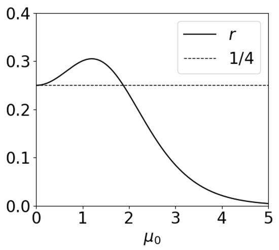
Figure 2. Function $r=r\left({\mu }_0\right)$ for the transmission and reflection on a ramp.

6. Solution to $\mathrm{𝒪}\left({\chi }^2\right)$

The main result of this work, to find a dispersion relationship to express $k=k_0+{\chi }^2{k}_1$ as a function of the wave angular velocity and the water depth while taking into account the varying bed, is presented in this section by solving the order $\mathrm{𝒪}\left({\chi }^2\right)$ of Equations (16)–(18).

6.1. Equations for $A_1$

In introducing Expansion (26) into the partial differential Equation (16) and retaining all the terms up to order $\mathrm{𝒪}\left({\chi }^2\right)$, and after some rearrangements,

$$\begin{array}{c}\stackrel{{\displaystyle I}}{\overbrace{-A_0{k}_0^2+{\displaystyle \frac{{\partial }^2{A}_0}{\partial z^2}}}}+{\chi }^2\left({\nabla }_{★}^2{A}_0-2A_0{k}_0{k}_1-A_1{k}_0^2+{\displaystyle \frac{{\partial }^2{A}_1}{\partial z^2}}\right)\hfill \\ \hfill \hspace{1em}\hspace{1em}\hspace{1em}\hspace{1em}\hspace{1em}\hspace{1em}\hspace{1em}\hspace{1em}\hspace{1em}\hspace{1em}\hspace{1em}\hspace{1em}\hspace{1em}\hspace{1em}\hspace{1em}\hspace{1em}\hspace{1em}\hspace{1em}\hspace{1em}\hspace{1em} -{\chi }^{-2}{A}_0{\displaystyle \frac{\partial {\theta }_0}{\partial z}}{\displaystyle \frac{\partial {\theta }_0}{\partial z}}=\mathrm{𝒪}\left({\chi }^4\right).\end{array}$$

(50)

The last term on the left-hand side includes $\partial {\theta }_0/\partial z=\mathrm{𝒪}\left({\chi }^2\right)$, so it is $\mathrm{𝒪}\left({\chi }^2\right)$ and is to be retained. Furthermore, according to the leading-order solution in Equation (30), the first two terms, $I=-A_0{k}_0^2+{\partial }^2{A}_0/\partial z^2$, cancel out if the are evaluated using $k_0$. However, we are to find the solutions using (and evaluating $A_0$ at) $k=k_0+{\chi }^2{k}_1$. A Taylor expansion gives

$$\begin{array}{c}I=-A_0\left(k=k_0+{\chi }^2{k}_1\right)k_0^2+{\displaystyle \frac{{\partial }^2{A}_0}{\partial z^2}}\left(k=k_0+{\chi }^2{k}_1\right)=\hfill \\ \hfill \hspace{1em}\hspace{1em}\hspace{1em}\hspace{1em}\hspace{1em}\hspace{1em}\hspace{1em}\hspace{1em}\hspace{1em}\hspace{1em}\hspace{1em}\hspace{1em}\hspace{1em} -A_0{k}_0^2+{\displaystyle \frac{{\partial }^2{A}_0}{\partial z^2}}-{\chi }^2{k}_1{\displaystyle \frac{\partial A_0}{\partial k}}{k}_0^2+{\chi }^2{k}_1{\displaystyle \frac{\partial }{\partial k}}{\displaystyle \frac{{\partial }^2{A}_0}{\partial z^2}},\end{array}$$

(51)

where all the evaluations on the right-hand side are at $k_0$, so that $-A_0{k}_0^2+{\partial }^2{A}_0/\partial z^2=0$ on the right-hand side of Equation (51), and therefore,

$$I={\chi }^2\left(-{\displaystyle \frac{\partial A_0}{\partial k}}{k}_0^2+{\displaystyle \frac{\partial }{\partial k}}{\displaystyle \frac{{\partial }^2{A}_0}{\partial z^2}}\right)k_1,$$

(52)

with the evaluations of $A_0$ and its derivatives performed at $k_0$. Note, however, that the evaluations of these terms could also be carried out at $k=k_0+{\chi }^2{k}_1$, since they add terms that are, overall, $\mathrm{𝒪}\left({\chi }^4\right)$ and negligible.

Since $A_0=K_{c0}cosh{q}_0$, the above expression (52) is also, after manipulation,

$$I=2{\chi }^2{A}_0{k}_0{k}_1,$$

so that Equation (50) is also (recall that $\partial {\theta }_0/\partial z=\mathrm{𝒪}\left({\chi }^2\right)$, and thus, all the terms below are the same order)

$$-A_1{k}_0^2+{\displaystyle \frac{{\partial }^2{A}_1}{\partial z^2}}=-{\nabla }_{★}^2{A}_0+{\chi }^{-4}{A}_0{\displaystyle \frac{\partial {\theta }_0}{\partial z}}{\displaystyle \frac{\partial {\theta }_0}{\partial z}}.$$

The above corresponds to the terms $\mathrm{𝒪}\left({\chi }^2\right)$ of continuity Equation (16). In proceeding similarly with boundary conditions (17) and (18), the equations for $A_1$ are

$$\begin{array}{ccc}\hfill -A_1{k}_0^2+{\displaystyle \frac{{\partial }^2{A}_1}{\partial z^2}}& =-{\nabla }_{★}^2{A}_0-{\chi }^{-4}{A}_0{\displaystyle \frac{\partial {\theta }_0}{\partial z}}{\displaystyle \frac{\partial {\theta }_0}{\partial z}},\hspace{1em}\hspace{1em}\hspace{1em}\hspace{1em}\hfill & \hfill -h⩽z⩽0,\end{array}$$

(53)

$$\begin{array}{ccc}\hfill {\displaystyle \frac{\partial A_1}{\partial z}}& =-{\nabla }_{★}{A}_0·{\nabla }_{★}h,\hspace{1em}\hspace{1em}\hspace{1em}\hspace{1em}\hspace{1em}\hspace{1em}\hspace{1em}\hspace{1em}\hspace{1em}\hspace{1em}\hspace{1em} \hfill & \hfill z=-h,\end{array}$$

(54)

$$\begin{array}{ccc}\hfill -{\omega }^2{A}_1+g{\displaystyle \frac{\partial A_1}{\partial z}}& =g{K}_{c0}m{k}_1,\hspace{1em}\hspace{1em}\hspace{1em}\hspace{1em}\hspace{1em}\hspace{1em}\hspace{1em}\hspace{1em}\hspace{1em}\hspace{1em}\hfill & \hfill z=0,\end{array}$$

(55)

with

$$m={\mu }_{0}tanh{\mu }_{0}sinh{\mu }_0-sinh{\mu }_0-{\mu }_{0}cosh{\mu }_0.$$

(56)

Equations (53) and (54) will allow us to solve for $A_1$, and then $k_1$ will be obtained from Equation (55).

6.2. Analytical solutions for $\partial {\theta }_0/\partial z=0$

The forcing term including the squared $\partial {\theta }_0/\partial z$ in Equation (53) prevents analytical solutions to exist. For illustration and also practical purposes, it is useful to first introduce the solution of the problem ignoring this forcing term.

The gradient and the Laplacian of $A_0$ in Equations (53) and (54) are

$${\nabla }_{★}{A}_0={\displaystyle \frac{\partial A_0}{\partial h}}{\nabla }_{★}h,{\nabla }_{★}^2{A}_0={\displaystyle \frac{\partial A_0}{\partial h}}{\nabla }_{★}^{2}h+{\displaystyle \frac{{\partial }^2{A}_0}{\partial h^2}}{\left|{\nabla }_{★}h\right|}^2,$$

where $\partial A_0/\partial h$ and ${\partial }^2{A}_0/\partial h^2$ are known from Equations (39) and (40). Differential Equation (53) happens to have an analytical solution. Already imposing boundary condition (54), the solution is

$$\begin{array}{c}{\displaystyle \frac{A_1}{K_{c0}}}=\left(-{\displaystyle \frac{{\delta }_{s1}}{4}}{q}_0^2-{\displaystyle \frac{{\delta }_{s0}}{2}}{q}_0\right)cosh{q}_0{\displaystyle \frac{h{\nabla }_{★}^{2}h}{{\mu }_0^2}}\hfill \\ \hspace{1em}\hspace{1em}+\left({\displaystyle \frac{-2{\delta }_{c0}+{\delta }_{s1}}{4}}{q}_0+{\displaystyle \frac{{\mu }_0}{2}}\right)sinh{q}_0{\displaystyle \frac{h{\nabla }_{★}^{2}h}{{\mu }_0^2}}\\ \hspace{1em}\hspace{1em}\hspace{1em}+\left({\displaystyle \frac{-{ϵ}_{s1}+{ϵ}_{c2}}{4}}{q}_0^2+{\displaystyle \frac{-2{ϵ}_{s0}+{ϵ}_{c1}}{4}}{q}_0\right)cosh{q}_0{\displaystyle \frac{|{\nabla }_{★}{h|}^2}{{\mu }_0^2}}\\ \hspace{1em}\hspace{1em}\hspace{1em}+\left(-{\displaystyle \frac{{ϵ}_{c2}}{6}}{q}_0^3-{\displaystyle \frac{{ϵ}_{c1}}{4}}{q}_0^2+{\displaystyle \frac{-2{ϵ}_{c0}+{ϵ}_{s1}-{ϵ}_{c2}}{4}}{q}_0-{\displaystyle \frac{{\alpha }_{k_0}{\mu }_0}{2}}\right)sinh{q}_0{\displaystyle \frac{|{\nabla }_{★}{h|}^2}{{\mu }_0^2}}\\ \hfill \hspace{1em}\hspace{1em}\hspace{1em}\hspace{1em}\hspace{1em}\hspace{1em}\hspace{1em}\hspace{1em}\hspace{1em}\hspace{1em}\hspace{1em}\hspace{1em}\hspace{1em}\hspace{1em}\hspace{1em}\hspace{1em}\hspace{1em}\hspace{1em}\hspace{1em}\hspace{1em}\hspace{1em}\hspace{1em}\hspace{1em}\hspace{1em}\hspace{1em}\hspace{1em}\hspace{1em}+K_{c1}cosh{q}_0.\end{array}$$

(57)

This new contribution of $\mathrm{𝒪}\left({\chi }^2\right)$ to the velocity profile is not considered in the work by Ge et al. [29], and it is also different than the depth functions considered in Modified and Complementary MSEs [14,15,16]. Solving the horizontal variations om $K_{c1}$ (constant in z) in Equation (57) requires, just as in the leading order for $K_{c0}$, the use of energy Equation (23), even though, again as with the leading-order case, the dispersion relationship does not require this constant $K_{c1}$ to be solved. The wavenumber $k_1$ is obtained from Equation (55), i.e.,

$$k_1={\displaystyle \frac{1}{g{K}_{c0}m}}\left(-{\omega }^2{A}_1+g{\displaystyle \frac{\partial A_1}{\partial z}}\right),\mathrm{at} z=0,$$

(58)

or, using the leading-order dispersion relationship ${\omega }^2=g{k}_{0}tanh{\mu }_0$—allowed since the errors introduced in $k_1$ are $\mathrm{𝒪}\left({\chi }^2\right)$, i.e., $\mathrm{𝒪}\left({\chi }^4\right)$ in $k=k_0+{\chi }^2{k}_1$—and using the above solution (57) for $A_1$, after manipulation, we have

$$k_1=k_0\left(F_{1}h{\nabla }_{★}^{2}h+F_2{\left|{\nabla }_{★}h\right|}^2\right),$$

(59)

where $F_i$ denotes the expressions of ${\mu }_0$, which are shown in Appendix B and plotted in Figure 3. As anticipated, $K_{c1}$ is not involved in Equation (59) for $k_1$. By introducing the above into $k=k_0+{\chi }^2{k}_1$, we finally obtain

$$k=k_0\left(1+F\right),$$

(60)

where F, which can be seen as a correction factor due to the bed slope, is

$$F=F_{1}h{\nabla }^{2}h+F_2{|\nabla h|}^2.$$

(61)

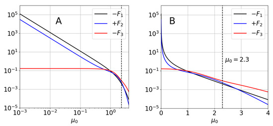
Figure 3. Functions $F_i=F_i\left({\mu }_0\right)$ for $i=1,2,3$ using log-log (A) and semi-log (B) scales. Dashed line is at ${\mu }_0=2.3$.

The proposed expression (60), with F in Equation (61), trivially reduces to the Burnside solution when ${\nabla }^{2}h=0$ and $|\nabla h|=0$, for flat beds. Functions $F_1$ and $F_2$, in Figure 3 ($-F_1$ shown, since $F_1<0$ and logarithmic scales are used), are so that $|F_i|<{10}^{-2}$ for ${\mu }_0\gtrsim 2.3$, decreasing exponentially as ${\mu }_0$ increases (Figure 3B). In other words, in deep waters, the dispersion relationship is not affected by the variations in the bed, as it is not by the depth itself. For practical purposes, we will consider that the influence of the slope is negligible for ${\mu }_0>2.3$.

On the other hand, for ${\mu }_0\lesssim 0.1$, the slope in the log–log plot (Figure 3A) is $-2$, i.e., both functions are $\propto {\mu }_0^{-2}$. Specifically, they are

$$F_1\sim -{\displaystyle \frac{1}{8{\mu }_0^2}},F_2\sim +{\displaystyle \frac{1}{32{\mu }_0^2}},\left[{\mu }_0\lesssim 0.1\right],$$

so that in shallow waters,

$$F\sim -{\displaystyle \frac{h{\nabla }^{2}h}{8{\mu }_0^2}}+{\displaystyle \frac{{|\nabla h|}^2}{32{\mu }_0^2}},\left[{\mu }_0\lesssim 0.1\right].$$

(62)

Given that the perturbative approximations are valid as long as the perturbation created, here F, is relatively small, say $\left|F\right|<F_c$ (a critic value), the above expression (62) also allows us to theoretically find the limit for the application of the present analysis in shallow waters. For the particular case of the bed being a sloped plane, when ${\nabla }^{2}h=0$, from the above expression,

$${\displaystyle \frac{|\nabla h|}{{\mu }_0}}\lesssim \sqrt{32F_c}\left\{{\displaystyle \frac{|\nabla h|}{{\mu }_0}}\lesssim 2.5 \mathrm{if} F_c\sim 0.2\right\}.$$

(63)

This condition has the same structure as the one for MSEs in Equation (2) and represents a significant increase in the validity domain. Also, for sloped planes, Figure 4 includes two relevant isolines for $F=F_2{|\nabla h|}^2$, showing the zone of present interest in the plane $\left\{|\nabla h|,{\mu }_0\right\}$, which corresponds to $0.001\lesssim F\lesssim F_c$ with $F_c\sim 0.2$; for $F>F_c$, the influence is too high, while for $F<0.001$, it can be considered negligible. The domain of the asymptotic result obtained by Ehrenmark [27] is illustrated in Figure 4 as ${\mu }_0⩽{10}^{-3}$, only as an indication to show that the domains are complementary. While both solutions recover the Burnside expression for $|\nabla h|=0$, no quantitative comparison is possible for small slopes since the solution of Ehrenmark is valid for infinitesimally small values of ${\mu }_0$, where the present theory has a singularity (except for flat beds).

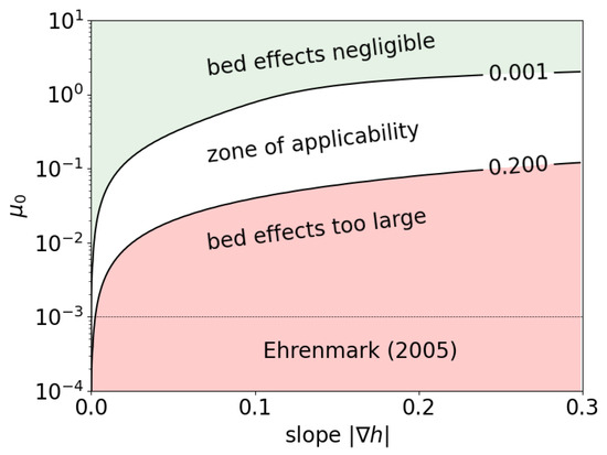
Figure 4. Sloped plane: isolines $0.2$ and $0.001$ for $F=F_2{|\nabla h|}^2$ (sloped plane).

For practical purposes, and although the exact expressions for $F_1$ and $F_2$ are provided in Appendix B, the simpler expressions

$$\begin{array}{cc}\hfill F_1& =-{\displaystyle \frac{exp\left(-0.315{\mu }_0^2-0.039{\mu }_0^3+0.013{\mu }_0^4\right)}{8{\mu }_0^2}}\hfill \end{array}$$

(64)

$$\begin{array}{cc}\hfill F_2& =+{\displaystyle \frac{exp\left(+2.430{\mu }_0^2-2.173{\mu }_0^3+0.641{\mu }_0^4-0.069{\mu }_0^5\right)}{32{\mu }_0^2}},\hfill \end{array}$$

(65)

provide approximations with errors below $0.5\%$ for the range of interest, i.e., $0⩽{\mu }_0⩽2.3$.

6.3. Numerical Solution for the General Case ($\partial {\theta }_0/\partial z\ne 0$)

In the general case, when $\partial {\theta }_0/\partial z$ is not null, i.e., recalling Equation (43), when $\nabla h·{\mathbf{s}}_{\mathbf{0}}\ne 0$, the system of Equations (53)–(55) has no analytical solutions for $A_1$. Now, the Equation (53) with bottom boundary condition (54) is to be solved numerically to obtain $A_1$, and $k_1$ is recovered from (55), also numerically. However, given the linear nature of the equations, it can be foreseen that the solution is still $k=k_0\left(1+F\right)$, now with

$$F=F_{1}h{\nabla }^{2}h+F_2{|\nabla h|}^2+F_3{\left(\nabla h·{\mathbf{s}}_{\mathbf{0}}\right)}^2,$$

(66)

where functions $F_1$ and $F_2$ are the ones presented above, and $F_3$, obtained numerically, is shown in Figure 3. In fact, in solving the system of equations numerically, $F_1$ and $F_2$ can also be estimated numerically, and they have been used to check the quality of the numerical integration and the overall validity of Expression (66). For the range of interest, $0⩽{\mu }_0⩽2.3$, the relative errors of the numerical estimations of $F_1$ and $F_2$, compared to the exact expressions, are below ${10}^{-6}$, which also guarantees the quality of the numerical estimation of $F_3$. The function $F_3$, included in Figure 3, can be again approximated in the range of interest through an exponential expression as

$$F_3=-{\displaystyle \frac{exp\left(-0.396{\mu }_0^2-0.143{\mu }_0^3-0.047{\mu }_0^4+0.034{\mu }_0^5\right)}{6}},$$

(67)

with errors below $0.5\%$ relative to the numerical solution. Function $F_3$ is non-negligible, when compared to $F_1$ and $F_2$, only for ${\mu }_0\gtrsim 0.3$ (see Figure 3A), i.e., where all $F_i$ are small and the influence of the bottom variations is expected to be nearly negligible.

6.4. Comparison to the Expression by Ge et al. [29]

The expression by Ge et al. [29], for sinusoidal bathymetries, is obtained using Fredholm’s alternative theorem (FAT) and by coupling the governing equation with the wave number and the varying seabed effects, without explicitly using perturbative approaches (see the original paper for details). Their equation is

$${\displaystyle \frac{{\omega }^2}{gk}}=\left(tanhkh+G_{1}h{\nabla }^{2}h+G_2{|\nabla h|}^2\right),$$

(68)

where

$$G_1\left(\mu \right)=-{\displaystyle \frac{\xi }{4\mu }},G_2\left(\mu \right)={\displaystyle \frac{{\xi }^2\left(9{\sigma }^2-{\mu }_1\mu +{\mu }_2{\mu }^2+{\mu }_3{\mu }^3+{\mu }_4{\mu }^4\right)}{12{\left(\sigma +\mu \xi \right)}^3}},$$

(69)

with $\sigma =tanh\mu$, $\xi =1-{\sigma }^2$, and

$$\begin{array}{cc}\hfill {\mu }_1& =12\sigma +9{\sigma }^3,\hfill \\ \hfill {\mu }_2& =9+45{\sigma }^2-18{\sigma }^4,\hfill \\ \hfill {\mu }_3& =28\sigma -78{\sigma }^3+30{\sigma }^5,\hfill \\ \hfill {\mu }_4& =10-40{\sigma }^2+42{\sigma }^4-12{\sigma }^6.\hfill \end{array}$$

Equation (68) can be rewritten in the same form as our Equation (60). First, note that $G_{1}h{\nabla }^{2}h$ and $G_2{|\nabla h|}^2$ are the small perturbations due to the bed shape, $\mathrm{𝒪}\left({\chi }^2\right)$. By following the perturbation theory procedures, we can assume that k is $k_0+{\chi }^2{k}_1+\mathrm{𝒪}\left({\chi }^4\right)$. In doing so, the above Equation (68) yields, with ${\mu }_0=k_{0}h$,

$$k_0={\displaystyle \frac{{\omega }^2}{gtanh{k}_{0}h}},$$

i.e., the Burnside equation, and

$${\chi }^2{k}_1=k_0{\displaystyle \frac{G_1\left({\mu }_0\right)h{\nabla }^{2}h+G_2\left({\mu }_0\right){|\nabla h|}^2}{{\mu }_0{tanh}^2{\mu }_0-tanh{\mu }_0-{\mu }_0}},$$

so that we can write (compare to Equations (60) and (61))

$$k=k_0\left(1+F_{1,G}h{\nabla }^{2}h+F_{2,G}{|\nabla h|}^2\right)+\mathrm{𝒪}\left({\chi }^4\right),$$

(70)

where

$$F_{i,G}={\displaystyle \frac{G_i\left({\mu }_0\right)}{{\mu }_0{tanh}^2{\mu }_0-tanh{\mu }_0-{\mu }_0}},i=1,2.$$

Note that, from Figure 5, and for $\mu \lesssim 0.3$, in spite of the different approaches considered, the results collapse for both $i=1,2$. However, the signs are opposite, i.e., $F_{i,G}\not\approx -F_i$.

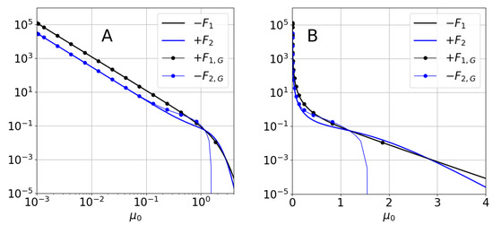
Figure 5. Functions $F_i=F_i\left({\mu }_0\right)$ and $F_{i,G}=F_{i,G}\left({\mu }_0\right)$ for $i=1,2$ using log-log (A) and semi-log (B) scales.

6.5. Numerical Checking of the Solution

The results for the second-order solution involve a considerable amount of algebra that deserves some kind of fully independent checking, especially after the results in Section 6.4. Here, we will numerically check the case of $\partial {\theta }_0/\partial z=0$, i.e., when an analytical solution is available (Section 6.2). We consider this case because the analytical solution simplifies the analysis, and at the same time, it includes the core of the work ($F_1$ and $F_2$, which dominate F, are obtained in this case). Additionally, we will consider a one-dimensional (1D) case for convenience and without loss of generality.

In recalling Equation (60), the second-order solution is

$$k=k_0+{\chi }^2{k}_1=k_0\left(1+F\right)=k_0\left(1+F_{1}h{h}_{xx}+F_2{h}_x^2\right),$$

(71)

where $F_1$ and $F_2$ have analytical expressions in Appendix B. From Equations (33) and (57) for $A_0$ and $A_1$, the second-order solution for A is the following; in recalling Section 6.1, note that the evaluations are performed particularly for $A_0$ and $K_{c0}$, using k and $q=k\left(z+h\right)$,

$$\begin{array}{c}A=A_0+{\chi }^2{A}_1=K_{c0}coshq+K_{c0}\left(-{\displaystyle \frac{{\delta }_{s1}}{4}}{q}^2-{\displaystyle \frac{{\delta }_{s0}}{2}}q\right)coshq{\displaystyle \frac{h{h}_{xx}}{{\mu }^2}}\hfill \\ \hspace{1em}\hspace{1em}\hspace{1em}+K_{c0}\left({\displaystyle \frac{-2{\delta }_{c0}+{\delta }_{s1}}{4}}q+{\displaystyle \frac{\mu }{2}}\right)sinhq{\displaystyle \frac{h{h}_{xx}}{{\mu }^2}}\\ \hspace{1em}\hspace{1em}\hspace{1em}\hspace{1em}+K_{c0}\left({\displaystyle \frac{-{ϵ}_{s1}+{ϵ}_{c2}}{4}}{q}^2+{\displaystyle \frac{-2{ϵ}_{s0}+{ϵ}_{c1}}{4}}q\right)coshq{\displaystyle \frac{h_x^2}{{\mu }^2}}\\ \hspace{1em}\hspace{1em}\hspace{1em}\hspace{1em}\hspace{1em}+K_{c0}\left(-{\displaystyle \frac{{ϵ}_{c2}}{6}}{q}^3-{\displaystyle \frac{{ϵ}_{c1}}{4}}{q}^2+{\displaystyle \frac{-2{ϵ}_{c0}+{ϵ}_{s1}-{ϵ}_{c2}}{4}}q-{\displaystyle \frac{{\alpha }_{k_0}\mu }{2}}\right)sinhq{\displaystyle \frac{h_x^2}{{\mu }^2}}\\ \hfill \hspace{1em}\hspace{1em}\hspace{1em}\hspace{1em}\hspace{1em}\hspace{1em}\hspace{1em}\hspace{1em}\hspace{1em}\hspace{1em}\hspace{1em}\hspace{1em}\hspace{1em}\hspace{1em}\hspace{1em}\hspace{1em}\hspace{1em}\hspace{1em}\hspace{1em}\hspace{1em}\hspace{1em}\hspace{1em}\hspace{1em}\hspace{1em}\hspace{1em}\hspace{1em}\hspace{1em}\hspace{1em}+K_{c0}{K}_{c1}coshq,\end{array}$$

(72)

where $K_{c0}$ is, from Equation (35),

$$K_{c0}={\displaystyle \frac{a}{\sqrt{sinh2\mu +2\mu }}},$$

where a is a constant representative of the deep-water wave amplitude.

The numerical checking is carried using the profile by Yu and Slinn [32], i.e.,

$$h=3.5tanh\left(-6{\displaystyle \frac{x}{l}}\right)-1.2{\displaystyle \frac{x}{l}}-2.5exp\left(-100{\left({\displaystyle \frac{x}{l}}+0.25\right)}^2\right),$$

where $x<0$. Figure 6 shows the profile for two different values of l; it is straightforward from the expression of the profile that changing l has the effect of stretching or shrinking in the horizontal axis direction, and it can be readily shown that, for constant $x_0/l$ (e.g., dashed lines in Figure 6), it is $h_x\propto l^{-1}$ and $h_{xx}\propto l^{-2}$, so that $l^{-1}$ plays the role of $\chi$ here.

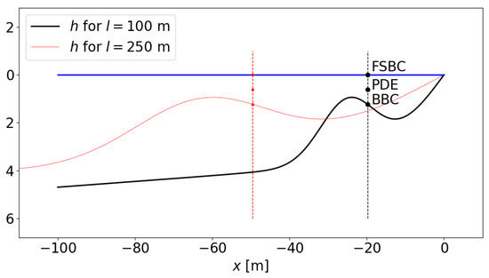
Figure 6. Yu and Slinn [32] profile for numerical checkings. FSBS: point to check the free-surface boundary condition; PDE: point to check the partial differential equation; BBC: point to check the bottom boundary condition.

The original conditions, prior to the use of WKB, the governing Equations (16)–(18) read as follows in 1D and ignoring $\partial \theta /\partial z$:

$$\begin{array}{ccc}\left(\mathrm{PDE}\right)\hfill & A_{xx}-A{k}^2+A_{zz}=0,\hspace{1em}\hspace{1em}\hfill & \hfill -h⩽z⩽0,\end{array}$$

(73)

$$\begin{array}{ccc}\left(\mathrm{BBC}\right)\hfill & A_x{h}_x+A_z=0,\hspace{1em}\hspace{1em}\hspace{1em}\hspace{1em} \hfill & \hfill z=-h,\end{array}$$

(74)

$$\begin{array}{ccc}\left(\mathrm{FSBC}\right)\hfill & -{\omega }^{2}A+g{A}_z=0,\hspace{1em}\hspace{1em}\hspace{1em}\hspace{1em}\hspace{1em}\hfill & \hfill z=0,\end{array}$$

(75)

where, as in Figure 6 and Figure 7, PDE = partial differential equation, BBC = bottom boundary condition, and FSBC = free-surface boundary condition. The correctness of the results is checked by introducing the above solutions (71) and (72) into a finite difference discretization of the governing Equations (73)–(75). To ensure that errors due to the finite difference discretization do not spoil the analysis, $\Delta x=\Delta z=0.01$ and very-high-order finite difference approximations are used, with truncation errors $\mathrm{𝒪}\left(\Delta x^8,\Delta z^8\right)$.

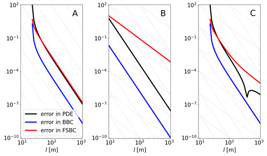
Figure 7. Evolution of the errors for equations using the proposed solutions. (A) Proposed solution (thin lines have slope $-4$, corresponding to $\mathrm{𝒪}\left(l^{-4}\right)$); (B) incorrectly using Burnside equation for k (thin lines have slopes $-2$ and $-4$); (C) using the proper k but introducing an error on purpose—${\delta }_{c0}=-1.01{\alpha }_{K_{c0}}$ instead of ${\delta }_{c0}=-{\alpha }_{K_{c0}}$ as it should according to Table 1 (thin lines have slopes $-2$ and $-4$).

According to the perturbative approach followed in this work, when introducing the obtained solutions in the original (raw) governing equations, there will be errors $\mathrm{𝒪}\left({\chi }^4\right)=\mathrm{𝒪}\left(l^{-4}\right)$ in all three equations (PDE, BBC, and FSBC), which correspond to unresolved orders—recall that $\partial \theta /\partial z=0$. Figure 7A shows how the errors do actually behave as expected—the evaluations are always performed at $x/l=-0.2$, as highlighted in Figure 6.

To illustrate how any change in the proposed solution can spoil it, making the convergence not be $\mathrm{𝒪}\left({\chi }^4\right)$, we consider two (wrong-on-purpose) cases. First, the Burnside solution $k_0$ is considered instead of $k=k_0\left(1+F\right)$ in all the equations involved; the result, in Figure 7B, shows that the convergence rate for both the PDE and the BBC is correct, but it is $\mathrm{𝒪}\left({\chi }^2\right)$ for the FSBC, precisely the equation from which k is derived. This emphasizes the well-known relevance of the free-surface boundary in obtaining the dispersion relationship. Finally, as shown in Figure 7C, if the result is considered to be ${\delta }_{c0}=-1.01{\alpha }_{K_{c0}}$ instead of ${\delta }_{c0}=-{\alpha }_{K_{c0}}$, as it should be according to Table 1, in this case, the convergence of both the PDE and FSBC is spoiled.

7. Two Cases of Application

Water wave propagation numerical models rely on depth-integrated equations such as the linear and fully dispersive MSEs (modified or not) or the nonlinear and weakly dispersive Boussinesq-type equations. These equations often neglect the effects of bottom variations or utilize velocity profile assumptions that differ from the solution presented in this study, and do not provide an expression for the corresponding dispersion equation. In using the new results presented here, particularly in Section 6 for $\mathrm{𝒪}\left({\chi }^2\right)$, the consequences of including (or neglecting) the bottom variations on the wave celerity are shown in this Section 7 with two one-dimensional (1D) examples—although the results provided here are valid for 2D cases. Both examples correspond to shallow-water conditions since, as already seen, the influence of the bed shape is negligible in deep waters.

7.1. Nearshore Propagation and Depth Inversion Problem

A first example deals with the propagation of wind-generated water waves as they approach the shore over a barred beach profile. We consider the propagation of linear waves with a period $T=7\mathrm{s}$ over the barred beach profile shown in Figure 8D, given by

$$h=3.5tanh\left(-6{\displaystyle \frac{x}{l}}\right)-1.2{\displaystyle \frac{x}{l}}-2.5exp\left(-100{\left({\displaystyle \frac{x}{l}}+0.25\right)}^2\right),$$

(76)

where $x<0$ and $l=100\mathrm{m}$. Note that this profile has relatively strong slopes to enhance the influence of the bottom variations; a more realistic case would consider $l>200\mathrm{m}$.

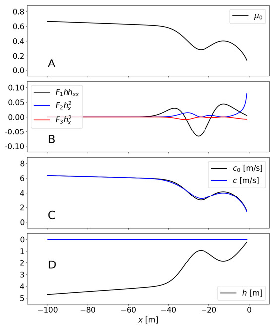
Figure 8. Wind-generated water waves of period $T=7\mathrm{s}$ propagation over a barred beach profile: evolution of ${\mu }_0$ (A), components of F (B), celerities $c_0$ and c (C) and water depth h (D).

The parameter ${\mu }_0=k_{0}h$, which is of paramount importance in the present analysis, is obtained from the leading-order dispersion equation and included in Figure 8A; it ranges from ∼0.6 in the offshore deepest zone to ∼0.3 over the bar and ∼0.2 in the shallower part. The factor F, which is required to obtain $k=k_0\left(1+F\right)$, reads in this 1D case

$$F=F_{1}h{h}_{xx}+F_2{h}_x^2+F_3{h}_x^2,$$

(77)

with $h_x=dh/dx$ and $h_{xx}=d^{2}h/d{x}^2$. Figure 8B shows the evolution of the three terms of the sum: the term $F_{1}h{h}_{xx}$ dominates over the bar, while $F_2{h}_x^2$ dominates very near the shore. As expected, the term $F_3{h}_x^2$ is generally small. The wave celerities $c_0=\omega /k_0$ and $c=\omega /k$ are shown in Figure 8C, with the differences reaching values up to $\pm 7\%$.

The above differences, due to F, have consequences on a relatively recent branch of algorithms for bathymetry estimation from video images. These algorithms, e.g., refs. [33,34,35] obtain the bathymetry from videos of the wave propagation in the shallow-water region, i.e., where the waves feel the bathymetry. For this purpose, these algorithms first obtain estimates of the wave period and the wavenumber using different techniques such as Fourier analysis or mode decomposition, and once $\omega$ and k have been estimated, all of them rely on the leading-order dispersion relationship to retrieve the water depth h.

Figure 9 is meant to illustrate the consequences of using the leading-order dispersion equation in bathymetric inversion methods, by simulating the type of errors that can be incurred when disregarding the slope $h_x$ and curvature $h_{xx}$ of the bottom. Figure 9 shows a bathymetry h, the same as in Figure 8D, the bathymetry retrieved using the leading-order dispersion equation (Burnside), and the wavenumber values obtained through the modified equation (i.e., the ones that would actually be observed). Linear waves of $T=7\mathrm{s}$ have again been considered. The maximum errors, i.e., the differences between the proposed bathymetry and the retried one are ∼20 cm in this case. If the characteristic length of the bathymetry, l, is increased to $200\mathrm{m}$ in Equation (76), i.e., in milder conditions, these errors are reduced to ∼5 cm. It should be noted that the bathymetric inversion algorithms have other difficulties related to the nonlinearity of the waves or the obliquity of the images that can be more relevant.

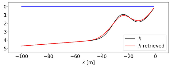
Figure 9. The inversion problem in a barred beach profile (h retrieved with the Burnside equation).

7.2. Tsunami Propagation over the Continental Slope

A second example is used to specifically show the influence of the slope, $h_x$, and also to show the limitations of the present analysis in very shallow waters. We consider the propagation of a tsunami over a continental slope as it travels to the shore. The continental slope is the abrupt rise from the ocean floor to the edge of the continental shelf. It marks the boundary between the continental shelf and the abyssal plain, and the slope angles typically range from $3^{\circ }$ to $6^{\circ }$ degrees (i.e., $0.05\lesssim |h_x|\lesssim 0.10$), reaching higher values in subduction zones. The idealized continental slope considered in this example has $|h_x|=0.075$, taking ∼25 km to go from a depth of $h=2000\mathrm{m}$ to $100\mathrm{m}$ (see Figure 10D). The junctions between the slope and flat zones (the abyssal plain and the continental shelf, respectively) have been smoothed over a length $l=4\mathrm{km}$ using polynomials that ensure the continuity of h, $h_x$, and $h_{xx}$. We initially consider the propagation of a tsunami with a wavelength $L=200\mathrm{km}$ in the deep zone; this would correspond, using the dispersion relationship, to a period of $T\sim 24$ min and a celerity, in the deep zone, of ∼500 km/h.

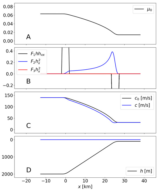
Figure 10. Tsunami propagation over a continental shelf: evolution of ${\mu }_0$ (A), components of F (B), celerities $c_0$ and c (C) and water depth h (D).

Figure 10 shows the most relevant results as in Figure 8. From Figure 10A, ${\mu }_0\lesssim 0.07$ in all the domain, with ${\mu }_0\sim 0.01$ in the shallower zone (continental shelf). Here, the values of ${\mu }_0$ are an order of magnitude smaller than in the previous example, which implies a more limiting condition on the maximum slope that can be handled. Figure 10B shows again the influence of each of the three terms summing up factor F in Equation (77). Owing to the way in which the bathymetry has been defined, $h_{xx}$ is null over the whole slope (except in the junction areas), and the term $F_{1}h{h}_{xx}$ is zero. Further, $F_3\ll F_2$ in the slope, as expected due to the small values of ${\mu }_0$ (Figure 3). In summary, the term $F_2{h}_x^2$ dominates the slope, with increasing values as the depth decreases and reaching values of ∼0.4. The impact on the wave celerity is shown in Figure 10C; the traveling time of the wave over the part of the slope where $h_{xx}=0$ is $231\mathrm{s}$ using $c_0$ and $262\mathrm{s}$ using the celerity c (i.e., $+13.1\%$).

Table 2 shows results obtained for the traveling time over the zone of the slope where $h_{xx}=0$ for different combinations of slope $|h_x|$ and wavelength L in the deep zone. The results show, quantitatively, that the greater the slope steepness and the longer the wavelength, the larger the differences in the traveling time become. At the same time, as the slope or the wavelength L increases, the maximum value of $\left|F\right|$ at that zone, ${\left|F\right|}_{\max }$, increases, and the condition ${\left|F\right|}_{\max }<F_c$ is violated. This is indicated with symbols in Table 2 (the results marked with † and ‡ should be regarded with caution). Tsunamis do usually have values of ${\mu }_0$ so small that even relatively small slopes of the continental shelf can violate the slope condition, both for the original condition in Equation (2), and also the new one in Equation (63). This point highlights the potential errors in tsunami propagation over the continental slope using depth-integrated models.

Table 2. Increment in traveling time over the slope (the zone where $h_{xx}=0$) using the modified dispersion relationship instead of using the leading-order relationship. The cases with ${0.2<\left|F\right|}_{\max }⩽0.4$ are marked with † (${\left|F\right|}_{\max }=$ maximum value of $\left|F\right|$ in the ramp), those with ${0.4<\left|F\right|}_{\max }⩽0.6$ with ‡, and those with ${\left|F\right|}_{\max }>0.6$ are ignored (—).

	L in the Deep Zone [km]
Slope $|{\mathbf{h}}_{\mathbf{x}}|$ [-]	10	50	100	200	500
$0.025$	$+0.0\%$	$+0.1\%$	$+0.5\%$	$+1.8\%$	$+11.4\%‡$
$0.050$	$+0.0\%$	$+0.4\%$	$+1.6\%$	$+6.4\%†$	—
$0.075$	$+0.0\%$	$+0.8\%$	$+3.2\%$	$+13.1\%†$	—
$0.100$	$+0.0\%$	$+1.3\%$	$+5.3\%$	$+21.5\%‡$	—
$0.150$	$+0.1\%$	$+2.5\%$	$+10.6\%†$	—	—
$0.200$	$+0.0\%$	$+4.1\%$	$+17.4\%†$	—	—

A second relevant aspect of Figure 10 is that the term $F_{1}h{h}_{xx}$ is dominant in the junction zones and, moreover, forces the violation of the condition $\left|F\right|<F_c$. Given that the condition is not satisfied, the results of the current theory cannot be applied to the junctions, and the behavior of the celerity remains unknown in that zone.

8. Concluding Remarks

This study explored the impact of the spatial variability in the seabed on key wave properties relevant to linear wave propagation employing a WKB approximation. Through solving the equations up to second-order $\mathrm{𝒪}\left({\chi }^2\right)$, where $\chi$ represents a characteristic value of the slope, two significant outcomes emerged.

Firstly, the well-established longwave theory governing linear transmission and reflection over a ramp was expanded to intermediate and deep waters. Secondly, and more prominently, a new dispersion relationship that incorporates the gradient and Laplacian of the mean water depth was derived. This resulting expression is readily applicable, and its implications for the problems of depth inversion and tsunami propagation are illustrated with two examples.

For the specific case of sloped planes, the analysis broadens the applicability range of the dispersion relationship over uneven bottoms from the classical mild-slope condition ($|\nabla h|\lesssim 0.38kh$) to an extended range ($|\nabla h|\lesssim 2.5kh$). Importantly, our findings underscore potential pitfalls associated with employing depth-integrated models under specific circumstances. The challenge posed by the tsunami propagation over the continental slope is a case that may surpass the validity of this study, clearly showing the influence of the Laplacian term.

References

- Mei, C.C. The Applied Dynamics of Ocean Surface Waves; World Scientific: Singapore, 1989. [Google Scholar]
- Dean, R.G.; Dalrymple, R.A. Water Wave Mechanics for Engineers and Scientists; World Scientific: Singapore, 1991. [Google Scholar]
- Svendsen, I.A. Introduction to Nearshore Hydrodynamics; Advanced Series on Ocean Engineering; World Scientific: Singapore, 2005. [Google Scholar]
- Kim, D.; Powers, T. Vertical integration of the Navier-Stokes equations for wave propagation in coastal waters. J. Fluid Mech. 2006, 566, 425–455. [Google Scholar]
- Chen, Q.; Kirby, J.T.; Dalrymple, R.A.; Kennedy, A.B.; Chawla, A. Boussinesq modeling of wave transformation, breaking, and runup. II: 2D. J. Waterw. Port Coast. Ocean Eng. 2000, 126, 48–56. [Google Scholar] [CrossRef]
- Mendez, F.J.; Losada, I.J. An empirical model to estimate the propagation of random breaking and nonbreaking waves over vegetation fields. Coast. Eng. 2004, 51, 103–118. [Google Scholar] [CrossRef]
- Infantes, E.; Orfila, A.; Simarro, G.; Terrados, J.; Alomar, C.; Tintoré, J. Effect of a seagrass (Posidonia oceanica) meadow on wave propagation. Mar. Ecol. Prog. Ser. 2012, 456, 63–72. [Google Scholar] [CrossRef]
- Mentaschi, L.; Besio, G.; Cassola, F.; Mazzino, A. Performance evaluation of Wavewatch III in the Mediterranean Sea. Ocean Model. 2015, 90, 82–94. [Google Scholar] [CrossRef]
- Airy, G.B. Tides and waves. Encycl. Metrop. 1845, 5, 241–396. [Google Scholar]
- Burnside, W. On the modification of a train of waves as it advances into shallow water. Proc. Lond. Math. Soc. 1915, s2_14, 131–133. [Google Scholar] [CrossRef]
- Stokes, G.G. On the theory of oscillatory waves. Trans. Camb. Philos. Soc. 1847, 8, 441–455. [Google Scholar]
- Berkhoff, J.C.W. Computation of combined refraction-diffraction. In Proceedings of the 13th Conference on Coastal Engineering, Vancouver, BC, Canada, 10–14 June 1972; Volume 2, pp. 471–490. [Google Scholar]
- Berkhoff, J.C.W. Mathematical Models for Simple Harmonic Linear Waves: Wave Diffraction and Refraction. Ph.D. Thesis, TU Delft, Delft, The Netherlands, 1976. [Google Scholar]
- Chamberlain, P.G.; Porter, D. The modified mild-slope equation. J. Fluid Mech. 1995, 291, 393–407. [Google Scholar] [CrossRef]
- Hsu, T.W.; Lin, T.Y.; Wen, C.C.; Ou, S.H. A complementary mild-slope equation derived using higher-order depth function for waves obliquely propagating on sloping bottom. Phys. Fluids 2006, 18, 087106. [Google Scholar] [CrossRef]
- Porter, R. An extended linear shallow-water equation. J. Fluid Mech. 2019, 876, 413–427. [Google Scholar] [CrossRef]
- Porter, D. The mild-slope equations: A unified theory. J. Fluid Mech. 2020, 887, A29. [Google Scholar] [CrossRef]
- Dingemans, M.W. Water Wave Propagation over Uneven Bottoms; World Scientific: Singapore, 1997. [Google Scholar] [CrossRef]
- Griffiths, D.J. Introduction to Fluid Mechanics, 1st ed.; Prentice Hall: Englewood Cliffs, NJ, USA, 1976. [Google Scholar]
- Boussinesq, J. Théorie des vagues propagées le long d’un canal ou d’une mer peu profonde. Comptes Rendus L’AcadéMie Des Sci. 1872, 74, 891–897. [Google Scholar]
- Peregrine, D.H. Long waves on a beach. J. Fluid Mech. 1967, 27, 815–827. [Google Scholar] [CrossRef]
- Liu, P.L.F. Model equations for wave propagation from deep water to shallow water. In Advances in Coastal and Ocean Engineering; World Scientific: Singapore, 1994; Chapter 3; pp. 125–158. [Google Scholar]
- Wei, G.; Kirby, J.T.; Grilli, S.T.; Subramanya, R. A fully nonlinear Boussinesq model for surface waves. Part 1: Highly nonlinear unsteady waves. J. Fluid Mech. 1995, 294, 71–92. [Google Scholar] [CrossRef]
- Simarro, G.; Orfila, A.; Galan, A. Linear shoaling in Boussinesq-type wave propagation models. Coast. Eng. J. 2013, 80, 100–106. [Google Scholar] [CrossRef]
- Nwogu, O. Alternative form of Boussinesq equations for nearshore wave propagation. J. Waterw. Port Coastal Ocean Eng. 1993, 119, 618–638. [Google Scholar] [CrossRef]
- Booij, N. A note on the accuracy of the mild-slope equation. Coast. Eng. 1983, 7, 191–203. [Google Scholar] [CrossRef]
- Ehrenmark, U. An alternative dispersion equation for water waves over an inclined bed. J. Fluid Mech. 2005, 543. [Google Scholar] [CrossRef]
- Williams, P.; Ehrenmark, U. A note on the use of a new dispersion formula for wave transformation over Roseau’s curved beach profile. Wave Motion 2010, 47, 641–647. [Google Scholar] [CrossRef]
- Ge, H.; Liu, H.; Zhang, L. Accurate depth inversion method for coastal bathymetry: Introduction of water wave high-order dispersion relation. J. Mar. Sci. Eng. 2020, 8, 153. [Google Scholar] [CrossRef]
- Dingemans, M.W. Water Wave Propagation over Uneven Bottoms. Ph.D. Thesis, Delft University of Technology, Delft, The Netherlands, 1994. [Google Scholar]
- Schäffer, H.A.; Madsen, P.A. Further enhancements of Boussinesq-type equations. Coast. Eng. 1995, 26, 1–14. [Google Scholar] [CrossRef]
- Yu, J.; Slinn, D. Effects of wave-current interaction on rip currents. J. Geophys. Res 2003, 108, 87. [Google Scholar] [CrossRef]
- Holman, R.; Bergsma, E.W.J. Updates to and performance of the cBathy algorithm for estimating nearshore bathymetry from remote sensing imagery. Remote Sens. 2021, 13, 3996. [Google Scholar] [CrossRef]
- Gawehn, M.; de Vries, S.; Aarninkhof, S. A self-adaptive method for mapping coastal bathymetry on-the-fly from wave field video. Remote Sens. 2021, 13, 4742. [Google Scholar] [CrossRef]
- Simarro, G.; Calvete, D. UBathy (v2.0): A software to obtain the bathymetry from video imagery. Remote. Sens. 2022, 14, 6139. [Google Scholar] [CrossRef]
Disclaimer/Publisher’s Note: The statements, opinions and data contained in all publications are solely those of the individual author(s) and contributor(s) and not of MDPI and/or the editor(s). MDPI and/or the editor(s) disclaim responsibility for any injury to people or property resulting from any ideas, methods, instructions or products referred to in the content. |
© 2024 by the author. Licensee MDPI, Basel, Switzerland. This article is an open access article distributed under the terms and conditions of the Creative Commons Attribution (CC BY) license (https://creativecommons.org/licenses/by/4.0/).