A Two-Step Approach for Evaluating the Dynamic Ultimate Load Capacity of Ship Structures

Abstract

One important parameter for evaluating the safety and reliability of a ship is o the dynamic ultimate load capacity of ship structures. Because of the importance of this parameter, its determination is essential. In this paper, a novel “two-step” approach for determining the dynamic ultimate load capacity of ship structures is proposed. The main idea of two-step approach is to determine the dynamic ultimate load capacity based on the static ultimate load capacity after accounting for impacts that cause strain on the ship structures. This approach is based on nonlinear finite element method. Here, taking stiffened plate as a case study, the practical application of thus two-step approach is discussed in detail. The results of this approach reveal that the static ultimate load capacity decreases by less than 3% after a stiffened plate is subjected to an impact load whose amplitude corresponds to the dynamic ultimate load capacity. Then, the influence of the impact duration on the failure mode and the effect of the impact load cycles and the impact load sequence on the dynamic ultimate load capacity of the stiffened plate were investigated. Finally, the applicability of the two-step approach to a hull girder is demonstrated. The two-step approach and the conclusions presented in this paper can provide guidance for the evaluation of dynamic ultimate load capacity.

1. Introduction

The ultimate load capacity of a ship is a crucial parameter for assessing its safety and reliability and has been extensively investigated by scholars. To date, numerous well-established methodologies have been developed to compute the static ultimate load capacity of ship structures. Smith [1] proposed an incremental-iteration method for calculating the ultimate load capacity of a hull girder. In this method, the cross-section is divided into different types of calculation units, each with its own specific stress–strain curve. By gradually increasing the curvature of the cross-section, calculating the stress of each unit, and integrating the stress of all units on the cross-section, one can obtain the bending moment-curvature curve where the peak value of the curve is the static ultimate load capacity of the hull girder. The curvature of the cross section refers to the angle at which the cross section of the hull girder rotates around the neutral axis. Because of its simplicity and high calculation accuracy, the incremental-iteration method has become a standard method for calculating the static ultimate load capacity of hull girders in classification societies. Tanaka et al. [2] extended the incremental-iteration method and established a method for calculating the ultimate load capacity of ship under combined bending and torsion, considering the influence of shear stress. Ueda and Sherif [3] proposed a numerical method called the Idealized Structural Unit Method (ISUM) for calculating the ultimate load capacity of ship structures. The structural units in the ISUM are larger than the elements in the finite element method (FEM), which greatly reduces the computation time [4]. Lindemann and Kaeding [5] used the ISUM to study the ultimate load capacity of the stiffened plates under lateral pressure and in-plane compression. Underwood et al. [6] proposed a new ISUM that can assess the static ultimate load capacity of damaged structures through collapse analysis of the stiffened plates.

In recent years, with the rapid improvement in computer performance, the nonlinear FEM has been widely used to compute the ultimate load capacity of ship structures. The nonlinear FEM is characterized by changes in structural stiffness in the FE analysis. There are three kinds of nonlinearity: geometric nonlinearity, material nonlinearity and boundary nonlinearity. The term “geometric nonlinearity” mainly refers to large deformations. The term “material nonlinearity” mainly refers to the consideration of the yield strength of the material. The term “boundary nonlinearity” mainly refers to changes in boundary conditions encountered during the analysis. It is common to encounter both geometric nonlinearity and material nonlinearity when analyzing ultimate load capacity. Thus, FE analysis is nonlinear. The ultimate load capacity of ship structures can be predicted by empirical formulas based on the numerous results obtained by the FEM. Zhang and Khan [7] proposed a semianalytical empirical formula and then performed numerical simulation of stiffened plates using FEM to determine the coefficients of the empirical formula. Kim et al. [8] proposed an empirical formula to predict the ultimate load capacity of the stiffened plates subjected to longitudinal compression through numerical calculations of the stiffened plates with T-bar and flat-bar stiffeners. Xu et al. [9] studied the effects of lateral pressure and stiffener types on the collapse behavior of the stiffened plates through nonlinear FEM and derived an empirical formula for predicting the ultimate load capacity of the stiffened plates under the combined actions of axial compression and different levels of lateral pressure based on the results of the numerical calculation.

In all of the above methods, the ultimate load capacity of ship structures is evaluated under static or quasistatic conditions. However, when a ship encounters extreme conditions such as large freak waves or underwater bubbles, the amplitude of the load on the ship is very large and the load duration can be reduced to the order of milliseconds [10,11]. Obviously, the load on ship structures cannot be considered as a static or quasistatic load in such situations. In particular, the incident report from MOL Comfort indicates that dynamic loads may be one of the causes of ship structure collapse [12]. Thus, it is meaningful to study the dynamic ultimate load capacity of ship structures. Yamada [13] studied the effect of strain rate on the ultimate load capacity of container ships by using a half-sinusoidal dynamic load. The numerical calculation revealed that the strain rate has a significant effect on the ultimate load capacity and that the ultimate load capacity could be increased by 10–20% when the strain rate was considered. Jagite et al. [14] found that in calculating the dynamic ultimate load capacity of ship structures subjected to wave loads, the effect of strain rate can be ignored for container ships. Yang et al. [15] studied the dynamic ultimate load capacity of rectangular plates under axial compression. These authors used the FE results for numerous ship plates to derive an empirical formula for predicting the dynamic ultimate compressive capacity of ship plates. Yang and Wang [16] studied the dynamic buckling of the stiffened plates under in-plane impact loads by theoretical derivation and considered the influence of rotational constraint stiffness on the dynamic response of the stiffened plates. Paik [17] studied the dynamic ultimate load capacity of plates under axial compression loads with different loading speeds. The experimental results show that as loading speed increases, the ultimate compressive capacity of the plate also increases gradually. Liu et al. [18] studied the dynamic failure of rectangular plates under lateral impact via impact experiments and FE analysis. Jagite et al. [19] studied the dynamic ultimate load capacity of the stiffened plates under axial compression and lateral load in a parameterized way. Load values obtained by parameterization are more consistent with those measured under real-world conditions. The limitations of the existing strain rate model are also discussed.

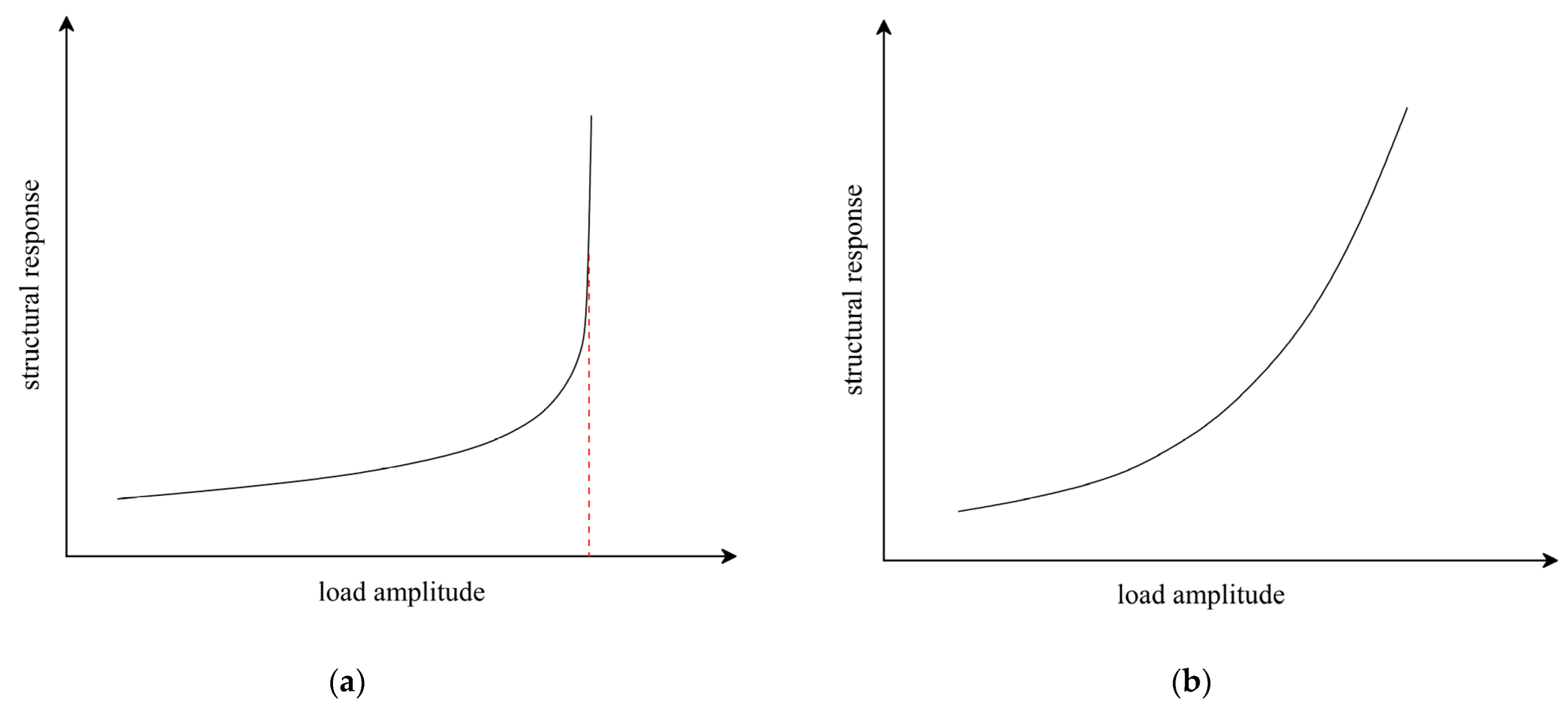
The current method for determining the dynamic ultimate load capacity of ship structures relies primarily on the concept of dynamic buckling. Ari-Gur and Simonetta [20] defined the dynamic failure criterion as the case in which a small increase in the dynamic load amplitude causes a sudden increase in the dynamic response of the structure. Xiong et al. [21] studied the dynamic ultimate compressive load capacity of the stiffened plates based on this criterion and derived a reasonably accurate empirical formula. Yang et al. [22] proposed a one-time thickness-deformation method for determining the dynamic ultimate load capacity by studying a container ship’s bow. Their formula defines the dynamic ultimate load capacity as the amplitude of the dynamic load at which the maximum deflection of the structure is equal to one times plate thickness. Yang and Wang [16] proposed a new formula for determining the dynamic critical buckling load. According to this formula, when the slope of the load-displacement curve at any given point reaches 35, the corresponding load at that point is the dynamic critical buckling load. There are other methods for determining the dynamic ultimate load capacity, but they are similar to those already described and will not be discussed further here. However, these methods all essentially use the deformation of the structure to determine the dynamic ultimate load capacity. There are drawbacks to applying these methods in some cases, as will be described below. Therefore, we hope to develop a novel method for determining the dynamic ultimate load capacity of ship structures.

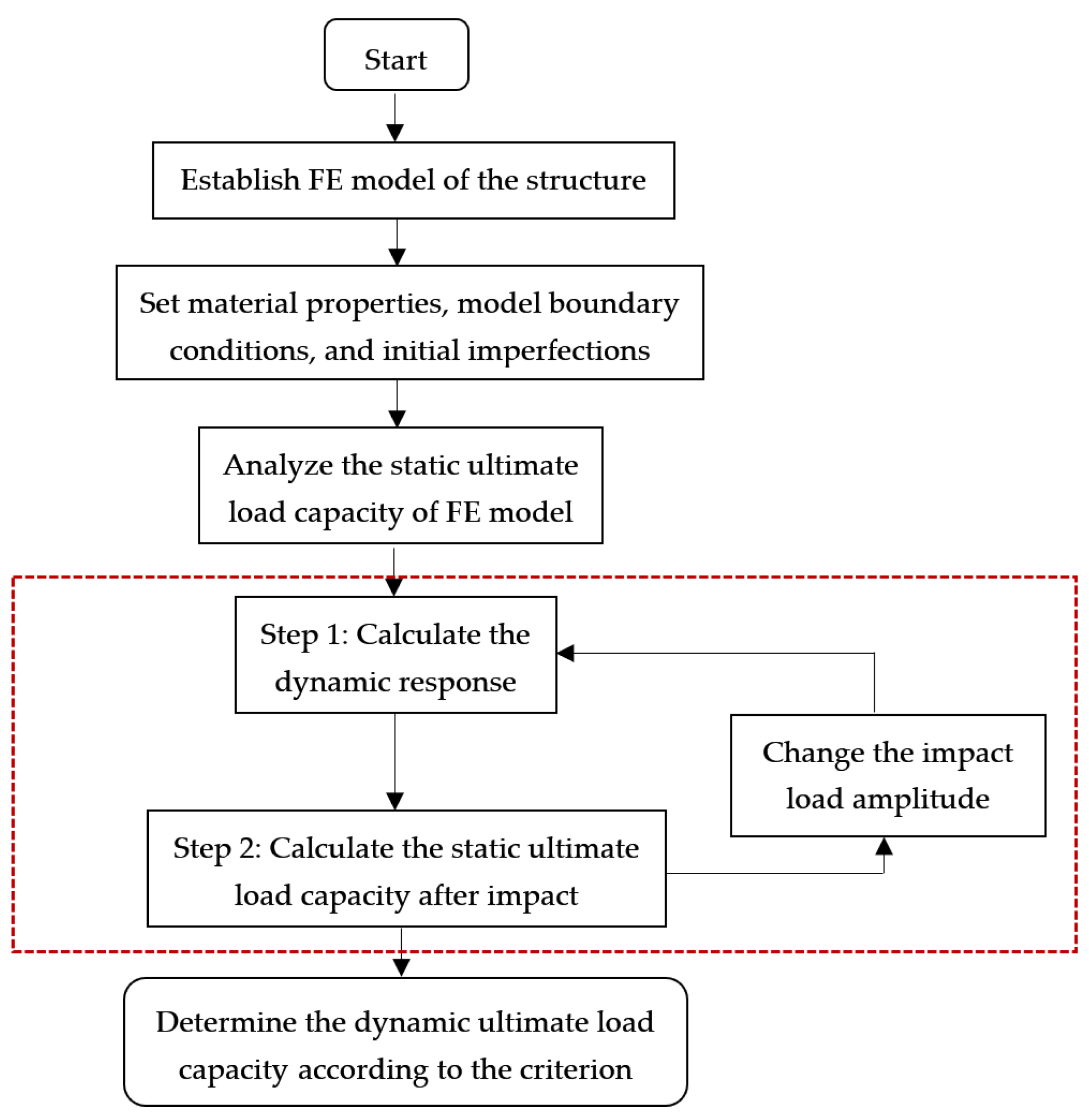
Considering the context described above, this study uses a nonlinear FEM to investigate the dynamic ultimate load capacity of the stiffened plates as one of the primary components of ship structures. This work proposes a novel “two-step” approach to determine the dynamic load capacity of the stiffened plates based on the static ultimate load capacity after impact. This method is theoretically applicable to a variety of ship structures. Subsequently, the failure mode of stiffened plates under impact load is discussed. Considering that real ship structures may experience continuous impacts with different load amplitudes, this work includes an analysis of the dynamic ultimate load capacity of the stiffened plates subjected to continuous impact load, as well as of the influence of the impact load cycles and impact load sequence on the dynamic ultimate load capacity of the stiffened plate. Finally, the applicability of the two-step approach to hull girders is studied.

2. Methodology

2.1. Two-Step Approach

The dynamic ultimate load capacity of the ship structure is usually determined by iterative methods, i.e., the duration of the dynamic load is fixed, and the maximum response of the structure is found by increasing the amplitude of the dynamic load. The response-amplitude curve is derived from these data, and the point on the curve where the slope changes fastest is the dynamic ultimate load capacity of the structure [21,23].

Jagite et al. [24] defined dynamic ultimate capacity as the maximum load that can be applied to the ship structure without causing structural collapse. When the impact duration is large, the dynamic ultimate load capacity becomes easier to calculate by the FEM. As the amplitude of the impact load increases, the structure begins to undergo large deformations (as shown in Figure 1a). The dynamic effect is not obvious at this time. However, when the duration of the impact load is relatively small, that is, when the impact duration is less than the natural vibration period of the structure, the response-amplitude curve of the structure is that shown in Figure 1b. Under those circumstances, the dynamic ultimate load capacity is difficult to determine.

This paper presents a novel “two-step” method for determining the dynamic ultimate load capacity of ship structures. The main idea of the two-step approach is to determine the dynamic ultimate load capacity of the ship structure by using the static ultimate load capacity after impact. After a ship structure is subjected to an impact load, the ship structure may exhibit plastic deformation. Too large a plastic deformation will reduce the static ultimate load capacity of the ship structure.

Step 1 of the two-step approach involves calculating the dynamic response of the ship structure under impact load, and step 2 of the two-step approach involves calculating the static ultimate load capacity after impact. Step 1 and step 2 are continuous, and step 2 completely inherits the deformation and stress state of the structure in step 1. It should be noted that step 2 is carried out after the dynamic response of the structure in step 1 becomes stable. The schematic diagram in Figure 2 illustrates the two-step process, using a stiffened plate as an example. The static ultimate load capacity of the stiffened plate is denoted as ${\sigma }_{u0}$, and the static ultimate load capacity after impact is ${\sigma }_{u\_i}$. In the application of the two-step approach, it is necessary to increase the amplitude of the dynamic load for continuous iterative calculation. In order to avoid including too many iterations, the static ultimate load capacity after impact is used to limit the number of iterations. In the process diagram, the static ultimate load capacity after impact cannot be less than 80% of the static ultimate load capacity, i.e., ${\sigma }_{u\_i}\ge 0.8{\sigma }_{u0}$. After the calculation is completed, two curves can be obtained: the curve of the peak value of dynamic response with the dynamic load amplitude and the curve of the static ultimate load capacity after impact with the dynamic load amplitude. The two-step approach to determining the dynamic ultimate load capacity will be discussed in detail in the third section.

The two-step approach uses the nonlinear FEM to determine the dynamic ultimate load capacity of a ship structure. As a mature method, the FEM is often used for structural analysis. The FEM for calculating the ultimate load capacity of ship structures is known to other researchers [25,26]. The details of the FEM-based process for determining the dynamic ultimate load capacity of a ship structure by the two-step approach are shown in Figure 3. As a basic ship structure, stiffened plates are studied by many scholars. For this reason, the procedures of the two-step approach and determining the dynamic ultimate load capacity are here illustrated via an analysis of a stiffened plate. In order to demonstrate that the two-step approach can be used to determine the dynamic ultimate load capacity of other ship structures, a hull girder is also studied.

2.2. FE Modeling of a Stiffened Plate

2.2.1. Geometric Data

Figure 4 shows the geometric properties of the stiffened plate, where x, y and z correspond to the longitudinal, transverse and vertical directions, respectively. The ‘1/2 + 1 + 1/2 bay & 1/2 + 1 + 1/2 span’ model was used in this study. According to the recommendation of ISSC 2012, using the longitudinal range of ‘1/2 + 1 + 1/2 span’ can bring the boundary conditions of the FE model close to the boundary conditions of a stiffened plate on a real ship, making the results of FE calculation more accurate. The length, the width, the width between stiffeners and the thickness of the stiffened plate are denoted as $a$, $B$, $b$ and $t_p$, respectively. A diagram of the cross-section of the T-bar stiffener is shown in Figure 5. The height and thickness of the stiffener’s web are denoted as $h_w$ and $t_w$, respectively. The width and thickness of the stiffener’s flange are denoted as $b_f$ and $t_f$, respectively. The geometric dimensions of the stiffened plate in this paper are shown in

Table 1. Geometric parameters of the stiffened plates.

Physical Quantity/Units	Symbol	Value
Plate length/mm	$a$	2550
Plate width/mm	$b$	850
Plate thickness/mm	$t_p$	11, 13, 16
Stiffener size 1/mm	$h_w\times b_f\times t_w/t_f$	138 × 90 × 9/12
Stiffener size 2/mm	$h_w\times b_f\times t_w/t_f$	235 × 90 × 10/15
Stiffener size 3/mm	$h_w\times b_f\times t_w/t_f$	383 × 100 × 12/17

. Three different sizes of plate thickness and stiffeners were used. The plate slenderness ratio is $\beta =b/t_p\cdot \sqrt{{\sigma }_y/E}$, and the stiffener slenderness ratio is $\lambda =a/\left(\pi r\right)\cdot \sqrt{{\sigma }_y/E}$, where $r=\sqrt{I/A}$ is the radius of gyration of the stiffener with full-width (b) plating. $A$ is the aero of the cross-section of the stiffener with full-width plating, and $I$ is moment of inertia of the stiffener with full-width plating. They are expressed as follows:

$$\begin{array}{l}A=b{t}_p+h_w{t}_w+b_f{t}_f\\ z_0=\left(\frac{{b{t}_p}^2}{2}+h_w{t}_w\left(t_p+\frac{h_w}{2}\right)+b_f{t}_f\left(t_p+h_w+\frac{t_f}{2}\right)\right)/A\\ I=\frac{{b{t}_p}^3+{h_w}^3{t}_w+{b_f{t}_f}^3}{12}+h_w{t}_w{\left(z_0-t_p-\frac{h_w}{2}\right)}^2+b_f{t}_f{\left(z_0-t_p-h_w-\frac{t_f}{2}\right)}^2+b{t}_p{\left(z_0-\frac{t_p}{2}\right)}^2\end{array}$$

(1)

2.2.2. Material Properties

The stiffened plates are made of high-tensile steel. The detailed material properties are as follows: Young’s modulus $E=2.06\times {10}^5\mathrm{MPa}$, Poisson’s ratio $\nu =0.3$, yield strength ${\sigma }_y=313.6\mathrm{MPa}$ and material density $\rho =7.85\times {10}^{-9}{ \mathrm{t}/\mathrm{mm}}^3$. The two-step approach requires calculation of the dynamic response of the stiffened plates and consideration of the effect of strain rate on the yield strength of the material. The influence of strain rate on yield strength of the material satisfies the Cowper–Symonds equation [27]. The Cowper–Symonds equation is as follows:

$${\sigma }_{yd}={\sigma }_y\left(1+{\left(\frac{\overline{\epsilon }}{D}\right)}^{1/q}\right)$$

(2)

where ${\sigma }_y$ is the static yield stress, ${\sigma }_{yd}$ is the dynamic yield stress, $\overline{\epsilon }$ is the plastic strain rate, and $D$ and $q$ are constant parameters related to material properties. The effect of strain rates on materials was comprehensively summarized by Paik, based on a multitude of experimental results [28]. As the material used in this study is high-strength steel, the values of the constant parameters should be $D=3200 {\mathrm{s}}^{-1}$ and $q=5$.

2.2.3. Initial Imperfections

The initial imperfections caused by welding of the stiffened plate include deflection of the structure and welding residual stress, which reduce the ultimate load capacity of the structure. Because the residual stress has little effect on the ultimate load capacity of the stiffened plate [29,30,31], only the initial deflection of the stiffened plate was considered in the study. According to ISSC 2012 [32], three types of initial deflections were considered in this study: local deflection of the plate, overall deflection and tripping of the stiffener. The specific expressions are as follows:

The local deflection of plate, $w_{pl}$:

$$w_{pl}=A_0\sin \frac{m\pi x}{a}\sin \frac{\pi y}{b}$$

(3)

where $m$ is the number of longitudinal buckling half-wave of the local plate and $m$ is the minimum integer that satisfies the following criterion:

$$\frac{a}{b}\le \sqrt{m\left(m+1\right)}$$

(4)

$A_0$ is the deflection amplitude of the local plate. Smith et al. [33] summarized the amplitudes of initial deflection and divided them into three types:

$$A_0=\{\begin{array}{c}0.025{\beta }^2{t}_p\hspace{1em}\mathrm{for} \mathrm{slight} \mathrm{level}\\ 0.1{\beta }^2{t}_p\hspace{1em}\mathrm{for} \mathrm{average} \mathrm{level}\\ 0.3{\beta }^2{t}_p\hspace{1em}\mathrm{for} \mathrm{severe} \mathrm{level}\end{array}$$

(5)

The average level of initial deflection is used in this study.

The overall deflection, $w_o$:

$$w_o=B_0\sin \frac{\pi x}{a}\sin \frac{\pi y}{B}$$

(6)

The tripping of the stiffener, $w_s$:

$$w_s=C_0\frac{z}{h_w}\sin \frac{\pi x}{a}$$

(7)

where $B_0$ and $C_0$ are the amplitude of overall deflection and tripping of the stiffener, both of which were set to $0.0015a$.

The three types of initial deflection of the stiffened plate are shown in Figure 6.

2.2.4. Applied Loads and Boundary Conditions

The boundary conditions were based on ISSC 2012 [29]. The transverse frames and longitudinal girders were regarded as constraints and, for simplicity, were not included in the FE model of the stiffened plate, as shown in Figure 7. According to the function for the structure, the transverse frame intersection of C-C′ and B-B′ should restrict the z-direction displacement of plate nodes and the y-direction displacement of the stiffener nodes. The longitudinal girder intersection of A′-D′ and A″-D″ should restrict the z-direction displacement of the plate nodes. The detailed boundary conditions of the stiffened plate are shown in

Table 2. Boundary conditions.

Location	Boundary Conditions
$\mathrm{A}-\mathrm{A}‴$$\mathrm{and} \mathrm{D}-\mathrm{D}‴$	$R_y=R_z=0$$\mathrm{and} U_x=$ uniform
$\mathrm{A}-\mathrm{D}$$\mathrm{and} \mathrm{A}‴-\mathrm{D}‴$	$R_x=R_z=0$$\mathrm{and} U_y=$ uniform
$\mathrm{A}\prime -\mathrm{D}\prime$$, \mathrm{A}″-\mathrm{D}″$, $\mathrm{B}-\mathrm{B}\prime$$\mathrm{and} \mathrm{C}-\mathrm{C}\prime$	$U_z=0$$\mathrm{at} \mathrm{plate} \mathrm{nodes}, U_y=0$ at stiffener nodes

.

The axial impact load can be simplified as a force load, and it can be described by a half-sinusoidal function. The amplitude curve of the impact load is given by

$$P\left(t\right)=P_{\max }\sin \left(\frac{\pi t}{T_d}\right)$$

(8)

where $P_{\max }$ is the maximum value of the impact load and $T_d$ is the duration of the impact load. The curve of the impact load is shown in Figure 8.

2.2.5. Non-Linear FE Modeling

The numerical calculations in this study were conducted in Abaqus 2021. In the process of numerical calculation, Dynamic-Implicit was used in step 1, and Static-General was used in step 2. The element type of FE model is S4R, which is a four-node, double-curved shell. Each node of the element has six degrees of freedom. An FE model of a typical stiffened plate is shown in Figure 9. The nodes at both ends are connected with the corresponding reference points by equation constraints to ensure that the displacements of the reference points and the nodes at both ends are equal in the x direction. In step 1, dynamic impact loads were applied to the reference points; in step 2, forced displacements were applied to the reference points.

3. Numerical Results and Discussion

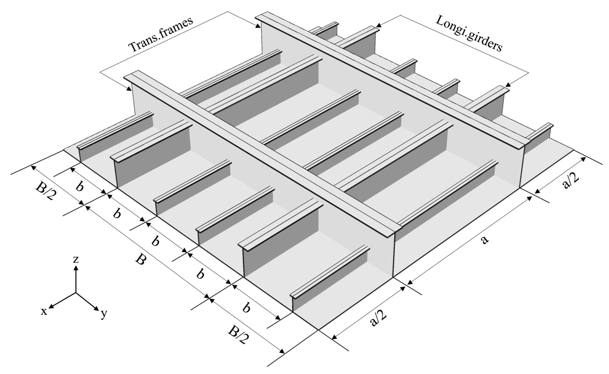
The purpose of this study is to propose a new method for determining the dynamic ultimate load capacity of ship structures. In order to make this method more universal, five different sizes of the stiffened panels were designed according to Table 1, as shown in

Table 3. Calculation model parameters.

Model	Thickness of the Plate (mm)	Size of the Stiffener	The Plate Slenderness Ratio $\mathit{\beta }$	The Stiffener Slenderness Ratio $\mathit{\lambda }$
Model 1	11	Size 1	3.02	0.65
Model 2	11	Size 2	3.02	0.36
Model 3	11	Size 3	3.02	0.21
Model 4	13	Size 2	2.55	0.38
Model 5	16	Size 2	2.07	0.40

. Zhang and Khan [34] found that the plate slenderness ratio $\beta$ ranges from 1.0 to 4.5 and that the stiffener slenderness ratio $\lambda$ ranges from 0.15 to 0.95 on ship structures. As shown in Table 3, the range of $\lambda$ and $\beta$ in the designed model are both within the range reported by Zhang and Khan.

3.1. Static Ultimate Load Capacity Results

Before calculating the dynamic ultimate load capacity, the static ultimate load capacity and the first-order vibration period of each model were calculated first. The impact load is determined by the impact duration and the impact load amplitude. Therefore, the static ultimate load capacity ${\sigma }_{u0}$ and the first-order vibration period $T_0$ can be used as the reference values for the amplitude of the impact load and the impact duration, respectively. Then, the nondimensional impact load amplitude and the nondimensional impact duration can be defined as $P_{\max }/{\sigma }_{u0}$ and $T_d/T_0$, respectively.

The accuracy of FEM can be verified by comparing the FE results with those of empirical formula, as discussed by Xiong et al. [21]. The results for static ultimate load capacity were verified by comparison with the empirical formula derived by Xu et al. [9]. This formula is relatively accurate for predicting the static ultimate load capacity of T-bar stiffened plates. The empirical formula is as follows:

$$\frac{{\sigma }_u}{{\sigma }_y}=\frac{1}{\sqrt{\left(\begin{array}{c}3.555-3.577\lambda -3.424\beta +0.999\lambda \beta +4.373{\lambda }^2+1.812{\beta }^2\\ -0.22{\lambda }^2{\beta }^2-2.584{\lambda }^3-0.277{\beta }^3+0.017{\lambda }^3{\beta }^3+0.458{\lambda }^4\end{array}\right)}}$$

(9)

The results for static ultimate load capacity of FEM, along with the empirical formula and errors, are shown in

Table 4. The results for static ultimate load capacity from FEM and the empirical formula, with errors.

Model	FEM	Empirical Formula	Error
Model 1	0.61	0.65	5.84%
Model 2	0.64	0.68	5.08%
Model 3	0.67	0.69	3.35%
Model 4	0.67	0.71	4.96%
Model 5	0.73	0.78	6.41%

. All error values are within 10%. The maximum error is 6.41%. Xiong et al. [21] compared the static ultimate load capacity obtained by FEM and the empirical formula. In that study, the maximum error was 7.14%, and all errors were within 10%. Thus, the results of the FEM calculation in this study are sufficiently precise.

3.2. The Determination Criterion of the Dynamic Ultimate Load Capacity

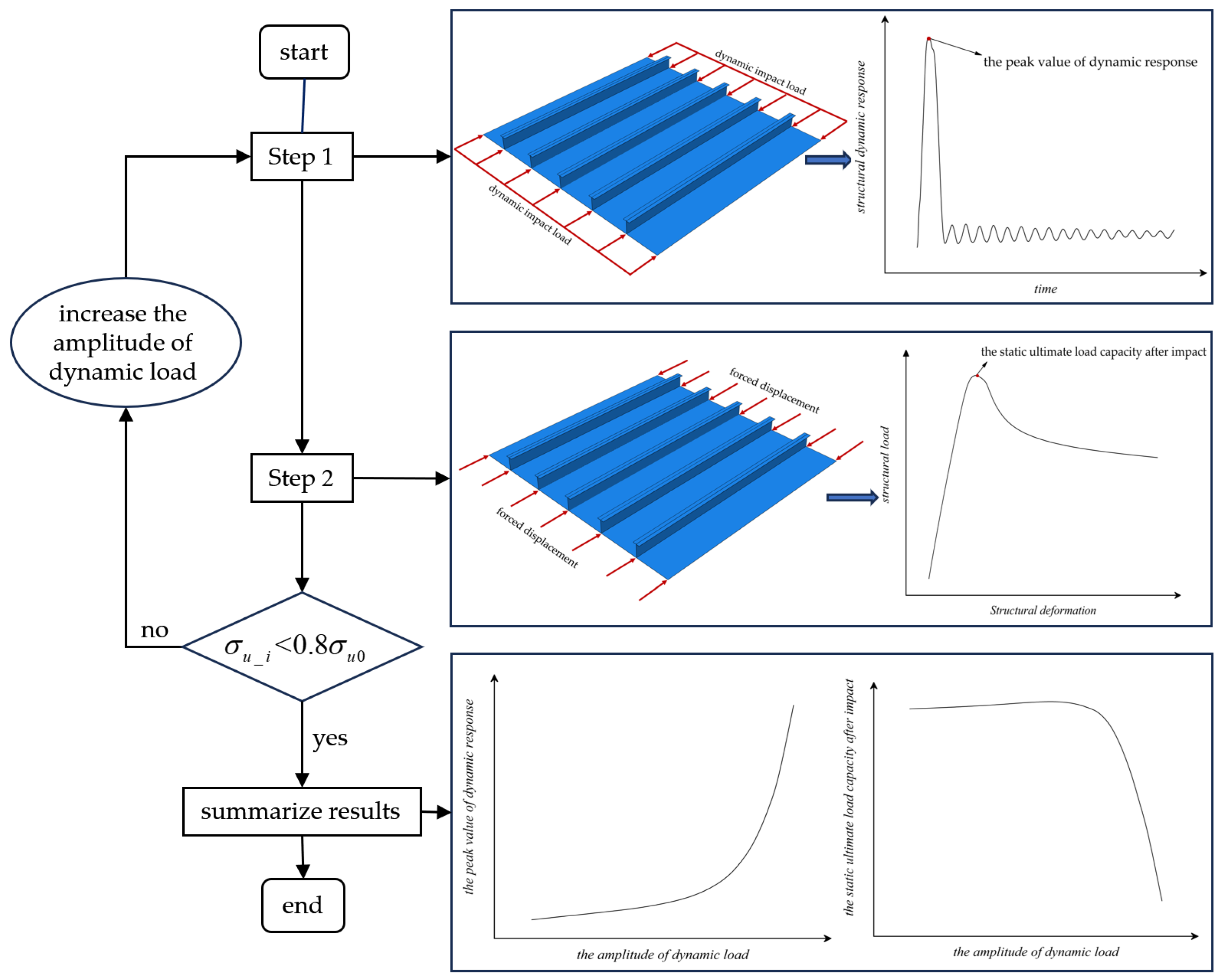
The dynamic ultimate load capacity of each stiffened plate model was computed based on the first vibration period, considering 5 different impact durations: 0.2T₀, 0.5T₀, T₀, 2T₀ and 5T₀. According to the calculation procedure of the two-step approach, the maximum value of the dynamic response of the stiffened plate was recorded in step 1, and then the static ultimate load capacity after impact was recorded in step 2. The peak value of the dynamic response is the maximum axial displacement of the loaded edge, i.e., $u_{\max }$. The maximum axial displacement of the stiffened plate under static ultimate load capacity is $u_{static}$. Thus, the nondimensional maximum axial displacement is defined as $u_{\max }/u_{static}$. The static ultimate load capacity of the stiffened plate after impact is denoted as ${\sigma }_{u\_i}$. The nondimensional static ultimate load capacity after impact is defined as ${\sigma }_{u\_i}/{\sigma }_{uo}$.

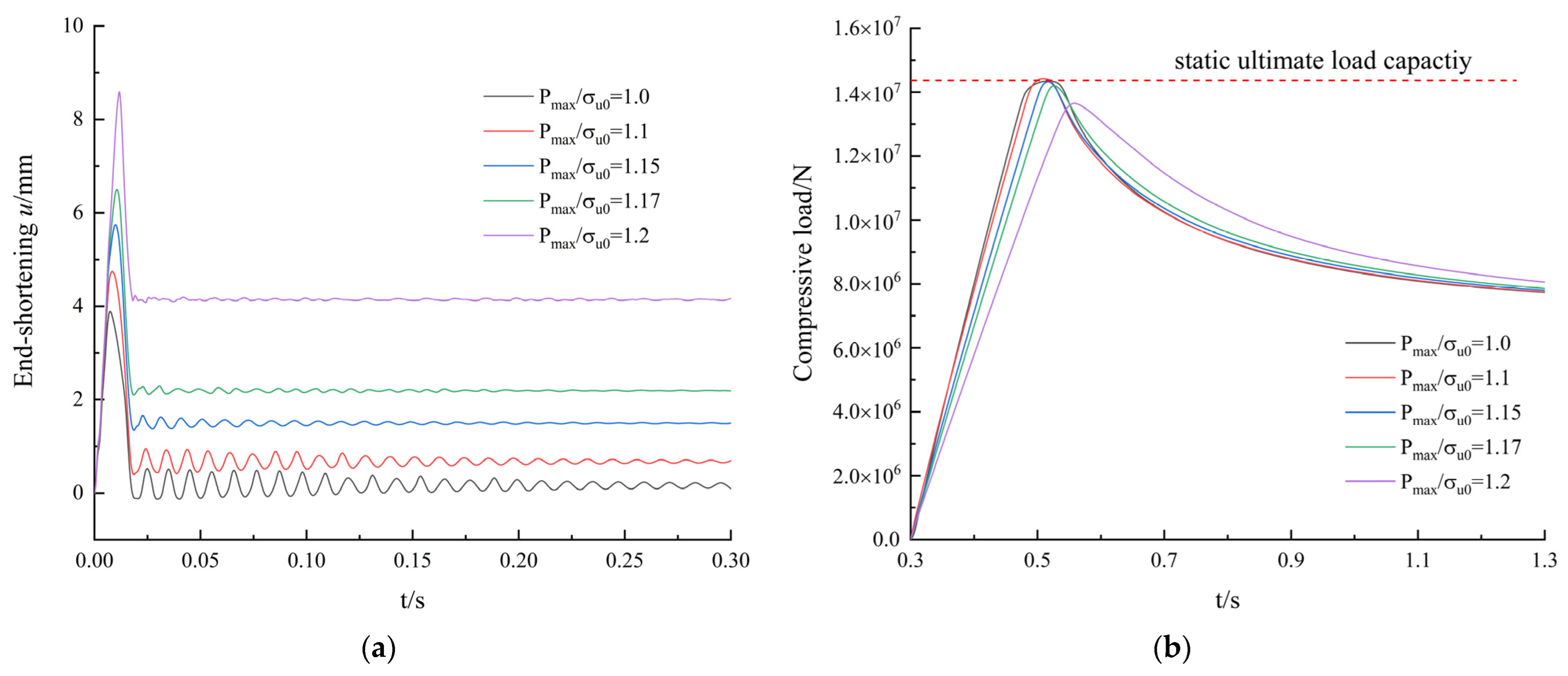
Model 3 was taken as an example to illustrate the calculation process in the two-step approach. The process of applying the two-step approach is similar to that used for other models. When the impact duration $T_d=T_0$, the results obtained by using the two-step approach are shown in Figure 10. The axial displacement of the stiffened plate over time subjected to impact loads with different amplitudes in step 1 is shown in Figure 10a. The axial displacement of the loaded edge can also be called “end shortening”. As shown in the figure, the stiffened plate vibrates after impact and then tends to stabilize. As load amplitude increases, the maximum axial displacement also increases gradually. When $P_{\max }/{\sigma }_{u0}=1.0$, the stiffened plate undergoes almost no plastic deformation after impact. However, when $P_{\max }/{\sigma }_{u0}>1.0$, the stiffened plate undergoes plastic deformation, and as the impact load amplitude increases, the plastic deformation of the stiffened plate increases gradually.

When the vibration of the stiffened plate becomes stable, the calculation in step 1 ends. The calculation in step 2 then begins, and forced displacement is applied at both ends of the stiffened plate to calculate the static ultimate load capacity. Figure 10b shows the compression load of the stiffened plate over time after impacts of different amplitudes. Note that step 1 was carried out in Dynamic-Implicit, with a total calculation time of 0.3 s, which is the real time. By contrast, step 2 was carried out in Static-General; in this step, the time is not real and defaults to 1 s. The maximum compressive load is the static ultimate load capacity after impact. It shown in Figure 10b that when $P_{\max }/{\sigma }_{u0}=1.0, 1.1, 1.15$, the static ultimate load capacity after impact ${\sigma }_{u\_i}$ does not decrease and is equal to the static ultimate load capacity ${\sigma }_{u0}$. However, when $P_{\max }/{\sigma }_{u0}=1.1, 1.15$, the structure undergoes plastic deformation, which indicates that low levels of plastic deformation have no influence on the static ultimate load capacity of the stiffened plates. As the impact load amplitude increases, the static ultimate load capacity after impact decreases obviously at $P_{\max }/{\sigma }_{u0}=1.2$.

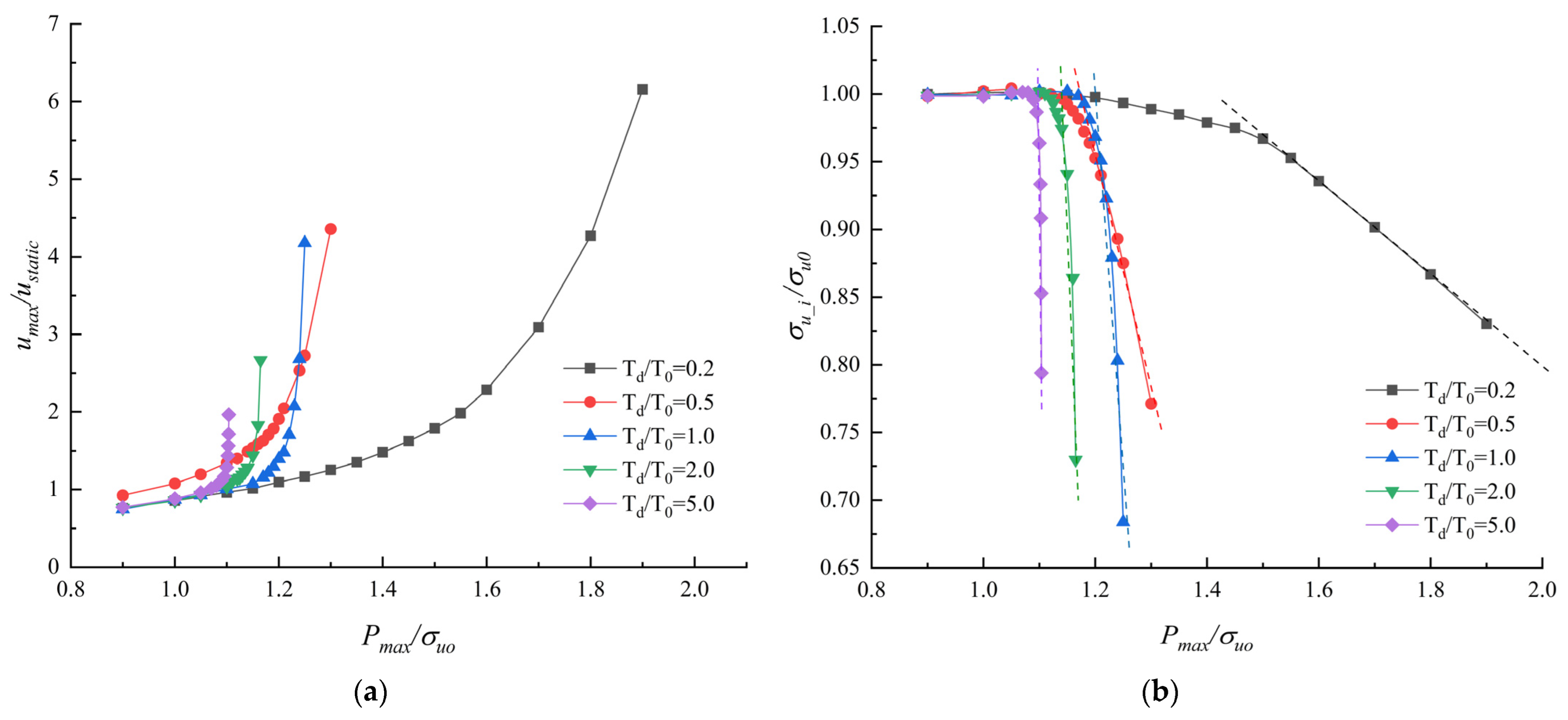
The curve of the nondimensional maximum axial displacement versus nondimensional load amplitude and the curve of nondimensional static ultimate load capacity after impact versus nondimensional load amplitude from Model 3 can be obtained by gradually, iteratively increasing the amplitude of the impact load for each impact duration. The results are shown in Figure 11.

By observing the trend in the maximum axial displacement versus the impact load amplitude in Figure 11a, we find that the maximum axial displacement gradually increases as the impact load amplitude increases and that the slope of the curve increases continuously. However, it shown in Figure 11b that the static ultimate load capacity after impact eventually stabilizes as the impact load amplitude increases, i.e., the static ultimate load capacity will not decrease after impact. Then, as the amplitude of the impact load continues to increase, the static ultimate load capacity after impact begins to decrease. The slope of the curve in Figure 11b is close to zero at the beginning, then begins to decrease; eventually, the slope becomes almost constant.

Therefore, we can find a point on the curve after which the slope of the curve remains constant, i.e., where the second derivative is 0, and define $P_{\max }/{\sigma }_{u0}$ of the point as the dynamic ultimate load capacity. The dynamic ultimate load capacity is denoted as ${\sigma }_{ud}$.

According to the above-described method of determining dynamic ultimate load capacity, the dynamic ultimate load capacity of Model 3 under different impact durations can be obtained, as shown in

Table 5. Dynamic ultimate load capacity and percentage reduction in static ultimate load capacity after impacts of different durations in Model 3.

${\mathit{T}}_{\mathit{d}}/{\mathit{T}}_0$	${\mathit{\sigma }}_{\mathit{u}\mathit{d}}/{\mathit{\sigma }}_{\mathit{u}0}$	$\left({\mathit{\sigma }}_{\mathit{u}\_\mathit{i}}-{\mathit{\sigma }}_{\mathit{u}0}\right)/{\mathit{\sigma }}_{\mathit{u}0}$
0.2	1.5	2.9%
0.5	1.18	1.9%
1.0	1.19	2.8%
2.0	1.14	2.6%
5.0	1.095	1.4%

. The percentage reduction of static ultimate load capacity after impact is given in the table. After the stiffened plate is subjected to the impact load whose amplitude is the dynamic ultimate load capacity, its static ultimate load capacity is reduced by 1.4–2.9%.

3.3. Dynamic Ultimate Load Capacity of Stiffened Plates

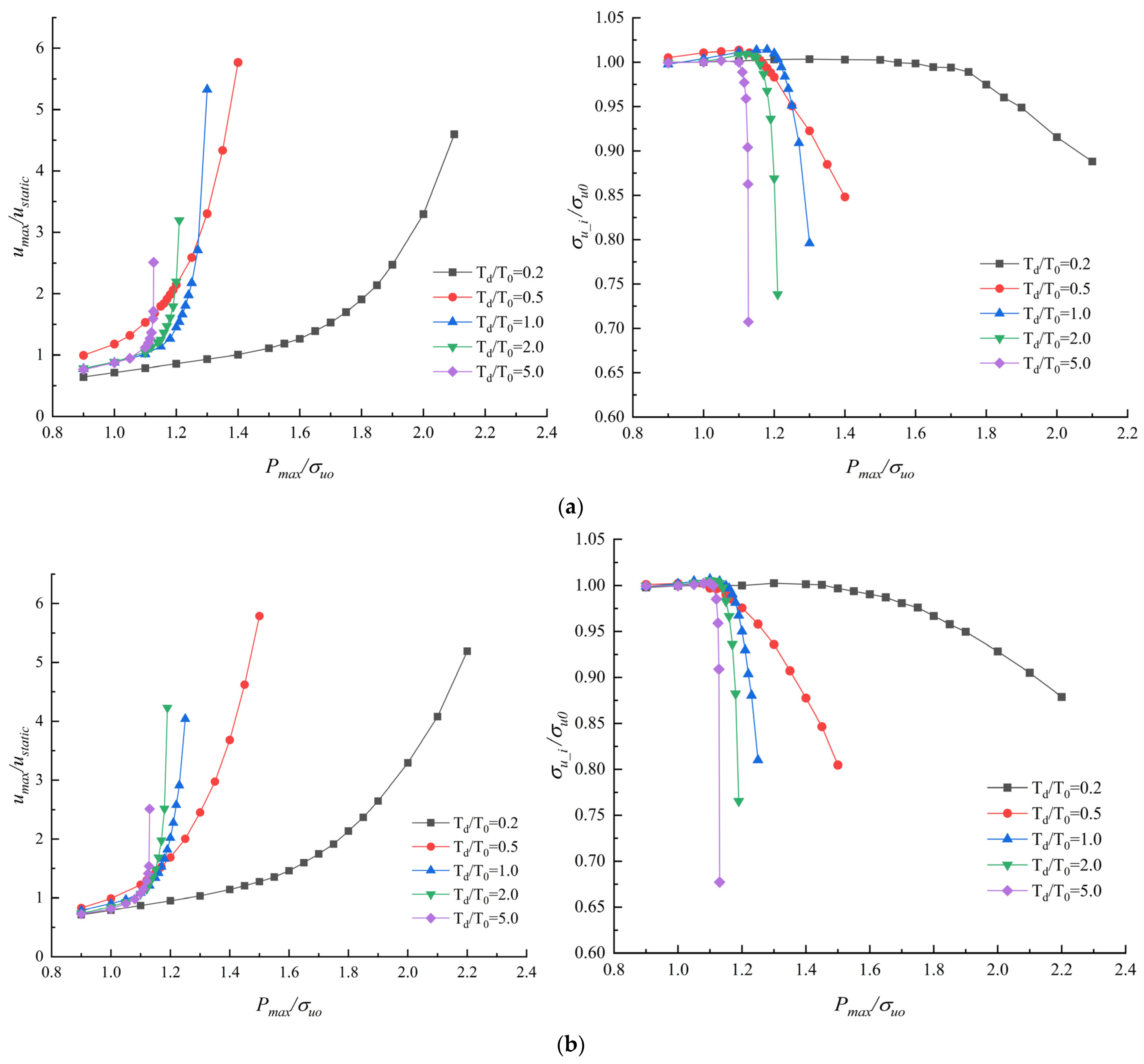
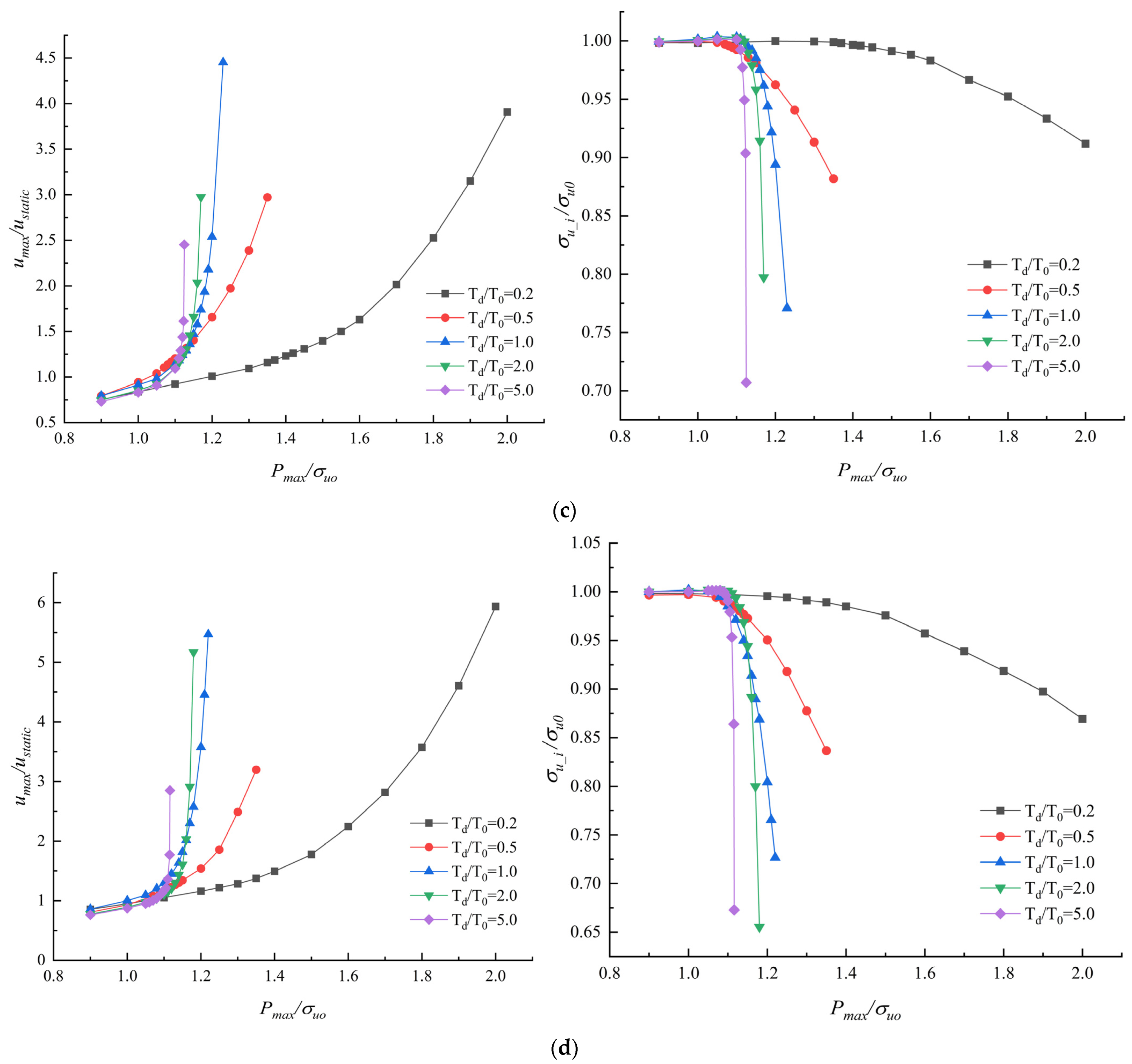
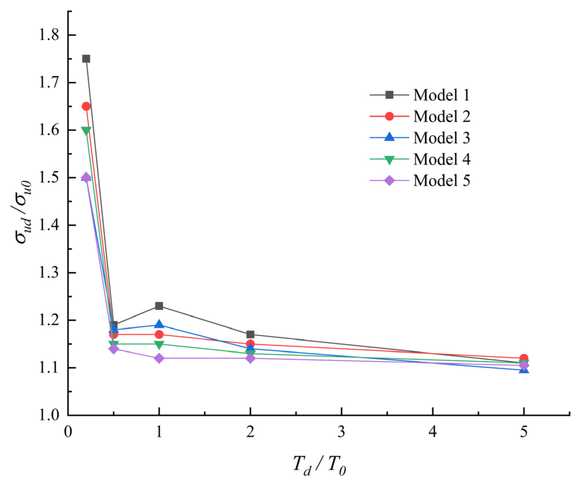
According to the procedure of the two-step approach, the calculation results from the other models are shown in Figure 12. The dynamic ultimate load capacity of each model under different impact durations is shown in Figure 13. As the impact duration increases, the dynamic ultimate load capacity of the stiffened plate gradually decreases. By observing the calculation results of Model 1 in Figure 13, we find that the dynamic ultimate load capacity is obviously smaller when $T_d/T_0=0.5$. Moreover, we observe the curve of the nondimensional maximum axial displacement versus nondimensional load amplitude of the stiffened plate in Figure 12a, and we find that the nondimensional maximum axial displacement corresponding to $T_d/T_0=0.5$ is the largest when $P_{\max }/{\sigma }_{u0}<1.1$. The cause of this phenomenon may be that higher-order deformation modes are activated under short impact duration. 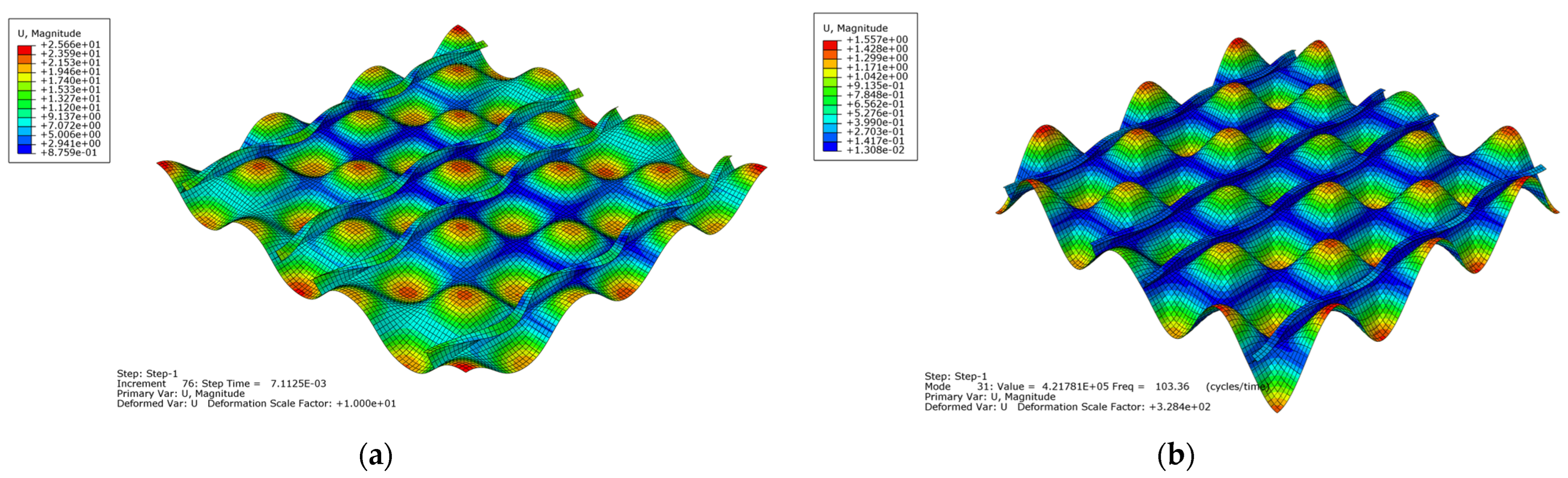Figure 14 shows the displacement distribution at dynamic ultimate state of Model 1 with $T_d=0.5T_0$ and the vibration mode with 103.36 Hz. As shown in Figure 14, the displacement distribution and vibration mode of the stiffened plate are similar. And the vibration period is about $0.48T_0$ when frequency is equal to 103.36 Hz, which is close to the impact duration $T_d=0.5T_0$. Therefore, when $T_d/T_0=0.5$, the impact load activates the high-order vibration mode of the stiffened plate, causing the resonance of the stiffened plate, thus the axial displacement of the stiffened plate increases significantly.

Table 6. The percentage reduction of static ultimate load capacity after impacts of different durations.

${\mathit{T}}_{\mathit{d}}/{\mathit{T}}_0$	Model 1	Model 2	Model 3	Model 4	Model 5
0.2	2.1%	1.7%	2.9%	1.7%	2.4%
0.5	1.2%	1.4%	1.9%	1.7%	2.4%
1	1.6%	1.0%	2.8%	1.6%	2.9%
2	1.4%	1.7%	2.6%	2.0%	1.6%
5	1.1%	1.5%	1.4%	1.0%	2.1%

shows the percentage reduction of static ultimate load capacity after impacts of different duration. The static ultimate load capacity of after impact all models is reduced by no more than 3%. It indicates that the static ultimate load capacity of the stiffened plate will decrease slightly when the stiffened plate is subjected to the impact load whose amplitude is the dynamic ultimate load capacity. We propose another method to determine the dynamic ultimate load capacity, that is, the static ultimate load capacity is reduced by 3% after the structure is subjected to the impact load, then the amplitude of this impact load is the dynamic ultimate load capacity. This method is suitable for the case where ship structures are subjected to impact loads of complex shapes.

3.4. Dynamic Failure Mode of Stiffened Plates

The failure mode of the stiffened plate can be divided into 6 types [34], as follows: mode I, overall failure mode; mode II, failure of the local plate between stiffeners; mode III, beam-column-type failure of the stiffeners with the attached plate; mode IV, local buckling of the stiffener web; mode V, tripping of the stiffener; mode VI, overall yielding of the stiffened plate. When stiffened plates are subjected to dynamic impact loads, the failure mode will change.

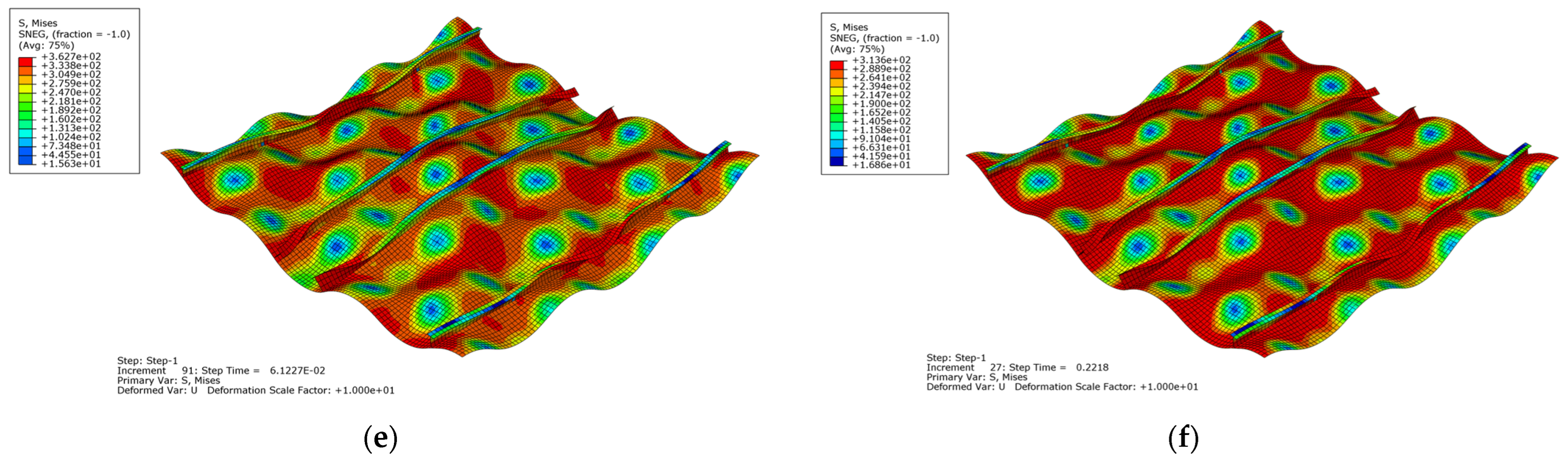
Figure 15 shows the stress diagram of Model 1 in the ultimate state. As shown in Figure 15a–e, the failure mode of the stiffened plate at the dynamic ultimate state changes as the impact duration increases. The failure mode of the stiffened plate is mainly failure of the local plate (mode II) when $T_d/T_0=0.2$. The deformation of the stiffener is relatively small. As the impact duration increases, both the tripping of the stiffener and the failure mode of the local plate arise when $T_d/T_0=0.5,1.0$, i.e., the failure modes are mainly mode II and mode V. The beam-column-type failure of the stiffened plate (mode III) is the main failure mode when $T_d/T_0=5.0$. In addition, the failure mode at this time is the same as the static failure mode of the stiffened plate in Figure 15f.

Figure 16 shows the stress diagram of Model 3 in the ultimate state. It can also be seen from Figure 16a–e that as the dynamic impact duration increases, the failure mode of the stiffened plate changes. The failure mode of the stiffened plate is mainly failure of local plate (mode II) when $T_d/T_0=0.2$. The deformation of the stiffener is very small. when $T_d/T_0=0.5,1.0$, the stiffener deformation increases, several half waves appear and the main failure modes are mode II and mode V. When $T_d/T_0=2.0,5.0$, the tripping of the stiffener (mode V) is the main failure mode. The failure mode in $T_d/T_0=5.0$ is the same as the static failure mode of the stiffened plate in Figure 16f.

In summary, the impact duration can affect the dynamic failure mode of the stiffened plate. The dynamic failure mode of the stiffened plate for $T_d/T_0=5.0$ is the same as the static failure mode.

3.5. Effect of the Number of Impact Load Cycles on Dynamic Ultimate Load Capacity

Figure 17 shows the schematic diagram of the impact load cycles: one cycle, two cycles and three cycles. Using the two-step approach, the dynamic ultimate load capacity of Model 2 under different numbers of impact load cycles is calculated when $T_d=T_0$. Figure 18 shows the calculation results obtained by the two-step approach. As shown in Figure 18a, the greater the number of impact cycles, the larger the maximum axial displacement of the stiffened plate under an impact load of the same amplitude. This effect occurs because the greater the number of impacts, the larger the load impulse applied to the stiffened plate and the larger the maximum axial displacement. Based on the results shown in Figure 18b, the dynamic ultimate load capacity under one impact, two impacts and three impacts can be determined as $1.18{\sigma }_{u0}$, $1.16{\sigma }_{u0}$ and $1.12{\sigma }_{u0}$, respectively. Therefore, the dynamic ultimate load capacity decreases as the number of impact cycles increases.

3.6. Effect of the Impact Load Sequence on Dynamic Ultimate Load Capacity

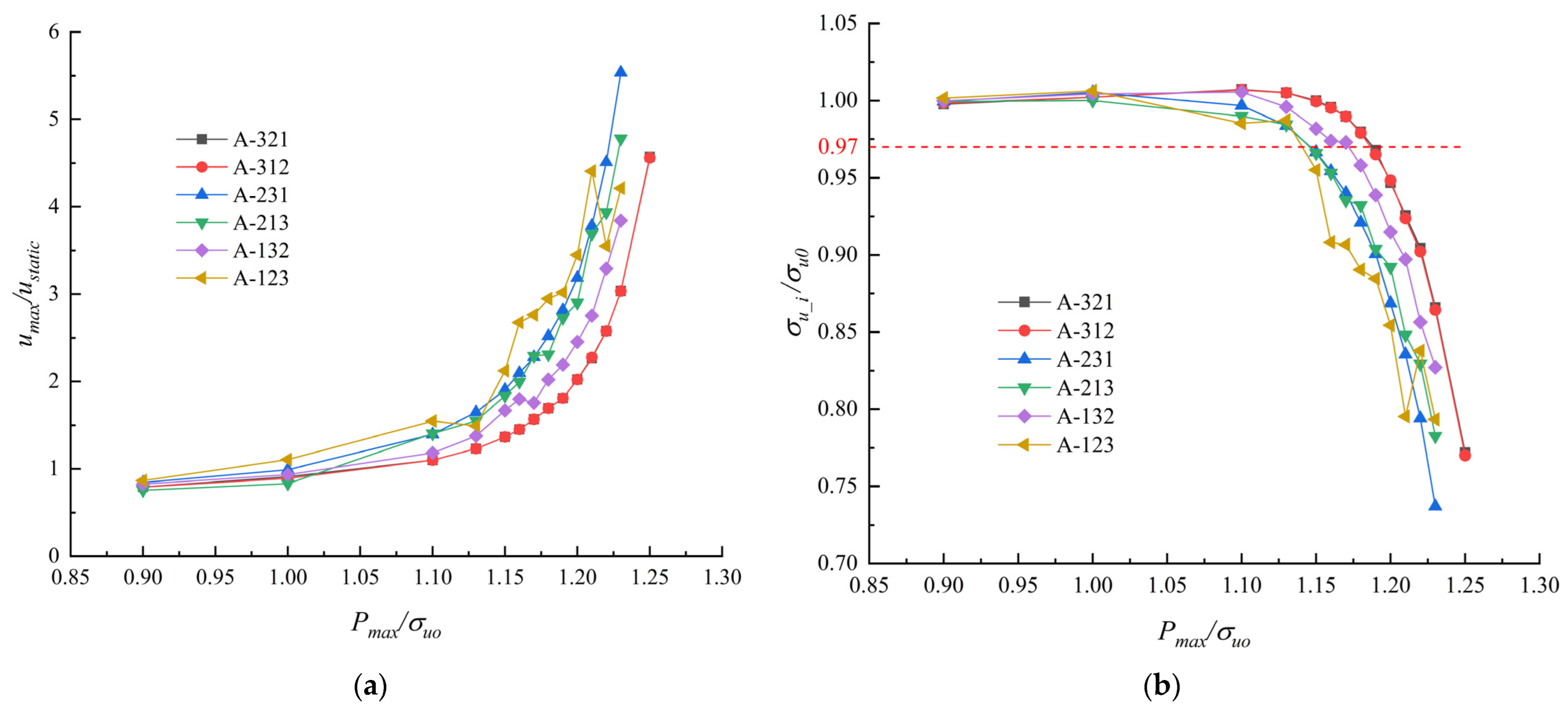
Real ship structures may be subjected to continuous impact loads with different amplitudes. Therefore, it is meaningful to study the dynamic ultimate load capacity of ship structures under continuous impact. We assume that the stiffened plate is impacted three times continuously, each time with different amplitudes. As shown in Figure 19, there are a total of six different sequences of the impact load s. The duration of each impact is denoted as $T_d$. The three amplitudes of the impact load are $0.4P_{\max }$, $0.6P_{\max }$ and $P_{\max }$, respectively. For ease of recording, the sequence of the impact load s is written as 1, 2, 3. For example, the sequence of the impact load amplitudes in Figure 19a is $0.4P_{\max }$, $0.6P_{\max }$, $P_{\max }$, which can be denoted as “A-123”.

With Model 2 as the case study and static ultimate load capacity as the reference value, the dynamic ultimate load capacity is calculated by using the two-step approach when $T_d=T_0$. The calculation results are shown in Figure 20. As higher-order modes may be activated, as observed in the course of continuous impacts, the curve of the nondimensional static ultimate load capacity after impact versus nondimensional impact load impact becomes non-smooth. The dynamic ultimate load capacity is derived from the percentage reduction in the static ultimate load capacity after the impact. According to the above discussion, the static ultimate load capacity after impact cannot be reduced by more than 3%, so we have chosen 3% reduction the criterion for determining the dynamic load capacity. Thus, results for different impact load sequences can be obtained, as shown in

Table 7. The dynamic ultimate load capacity of Model 1 under different load sequences.

Load Sequence	${\mathit{\sigma }}_{\mathit{u}\mathit{d}}/{\mathit{\sigma }}_{\mathit{u}0}$
A-321	1.185
A-312	1.185
A-231	1.147
A-213	1.147
A-132	1.17
A-123	1.14

. The 3% reduction is based on the nondimensional results from the five models of stiffened plates under five different impact times. Therefore, it is reasonable to take a 3% reduction as the criterion for determining the dynamic ultimate load capacity. When the last impact load is the one with the highest amplitude, i.e., when the load sequence is “A-123”, the dynamic ultimate load capacity of the stiffened plate is the smallest. Because the stiffened plate has been subjected to two impact loads with different amplitudes and then subjected to an impact load with a higher amplitude, the deformation and plastic region of the stiffened plate will be significantly larger than in other cases, reducing the dynamic ultimate load capacity. For comparison, when the load sequence is “A-321”, the highest-amplitude load occurs first. After that impact, the smaller loads are not able to expand the plastic region further. Additionally, plastic regions have already been generated when the smaller loads occur, resulting in smaller deformations and a greater ultimate load capacity.

3.7. Application of the Two-Step Approach to a Hull Girder

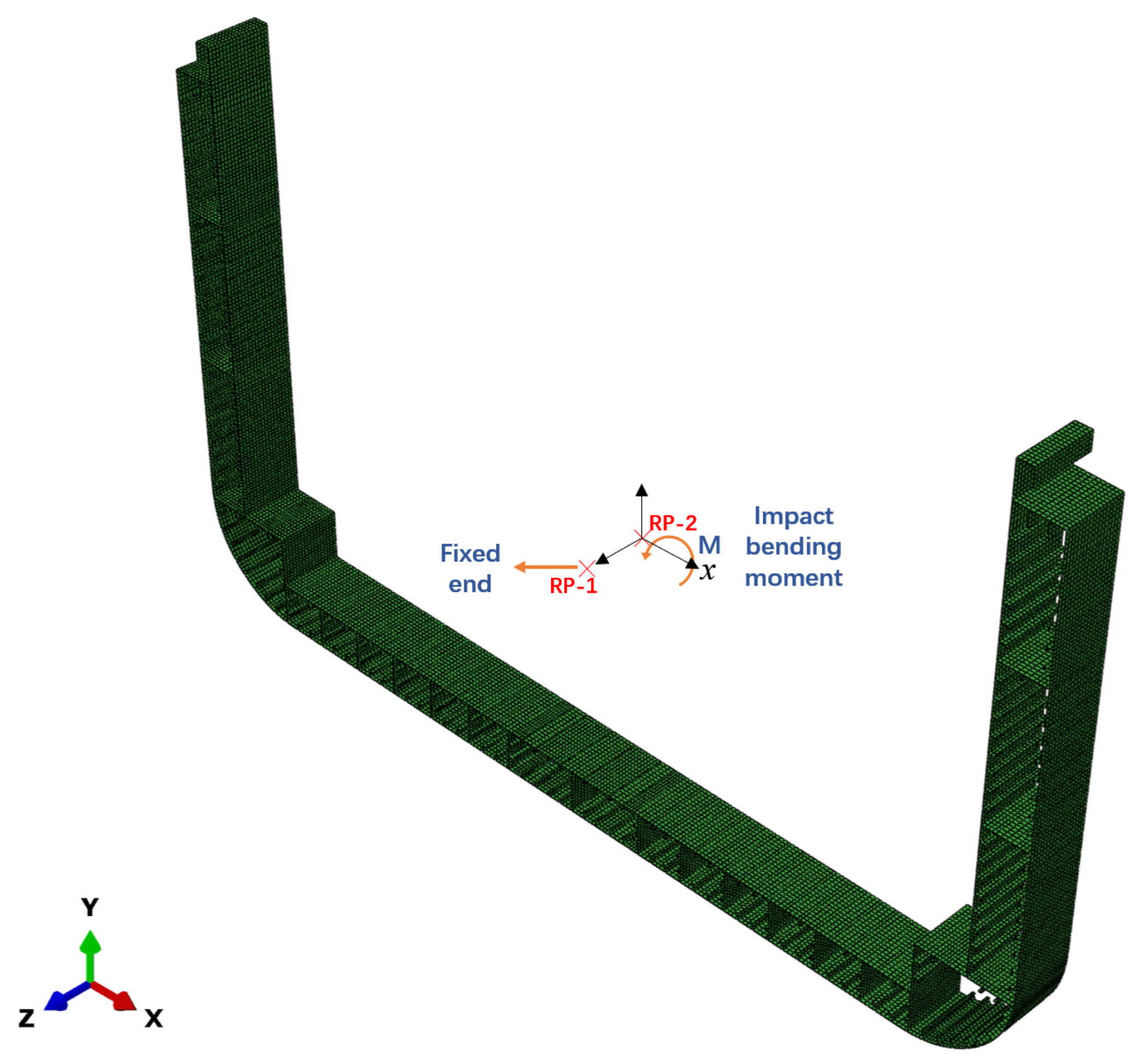
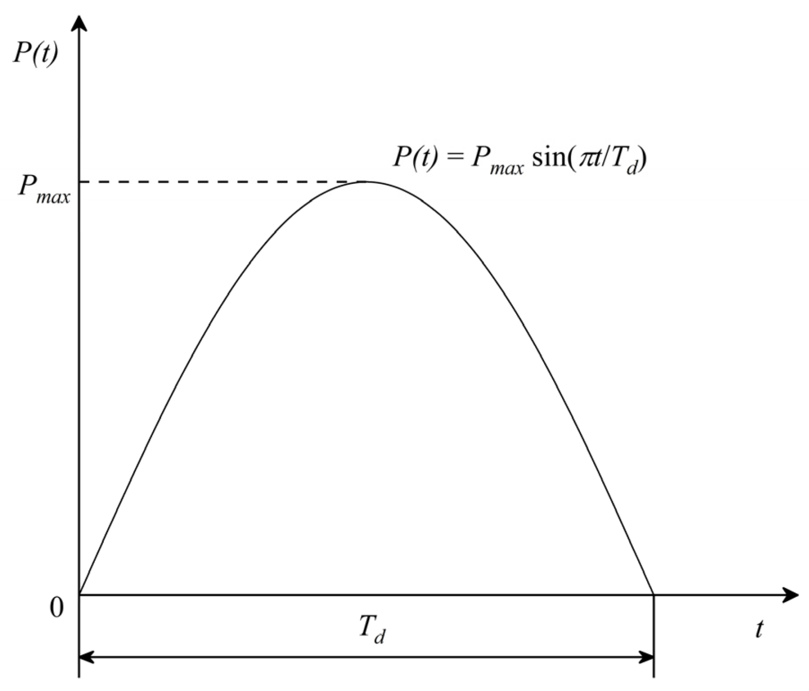
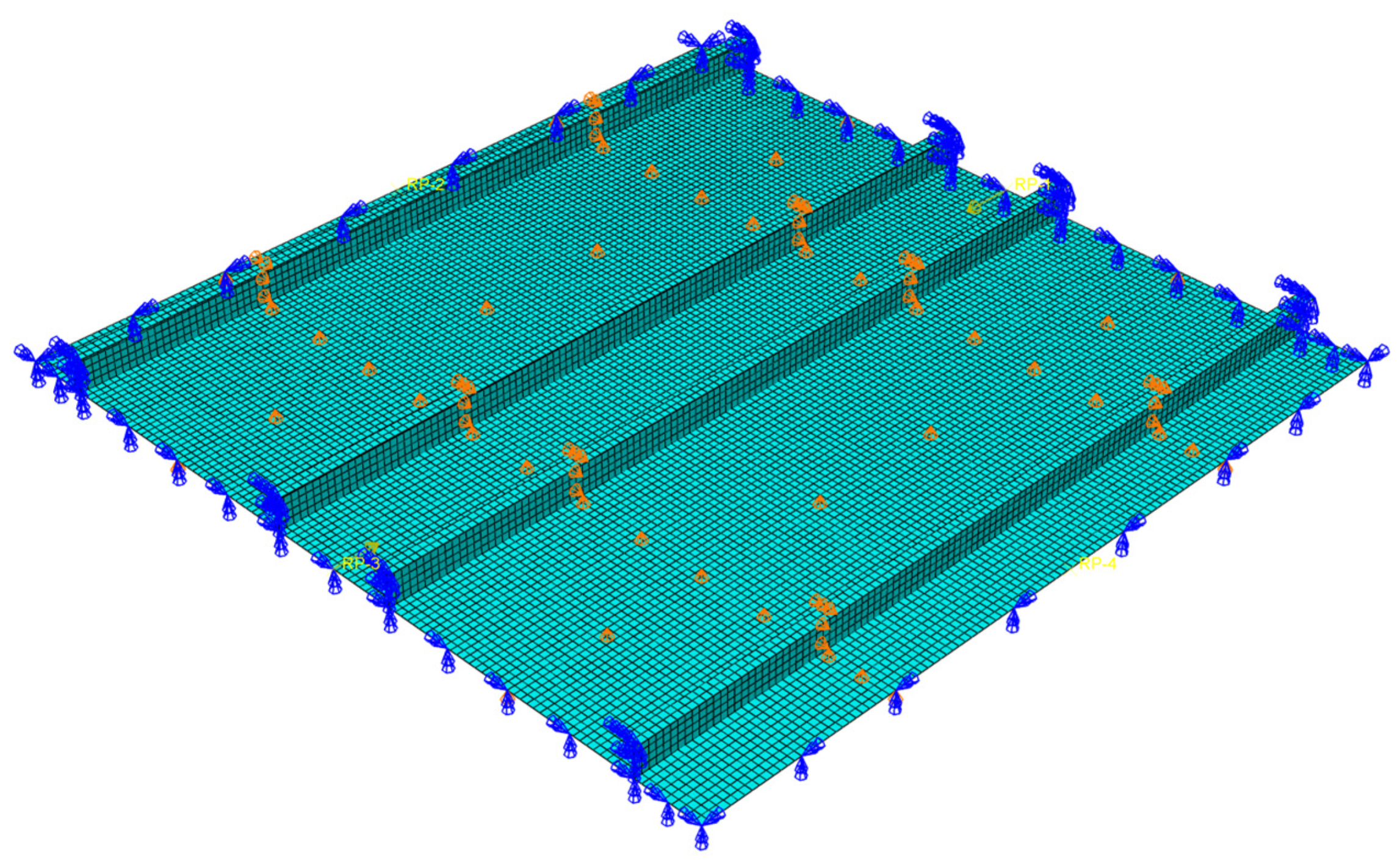
In order to illustrate the applicability of the two-step approach to other ship structures, the two-step approach was used to calculate the dynamic ultimate load capacity of a hull girder. Figure 21 shows the schematic diagram of a single-frame model of a container-ship hull girder. The two reference points (RP-1 and RP-2) and all nodes at both ends of the model are coupled by coupling constraints. Both the boundary conditions and the impact bending moment are applied to the reference points. One end of the model is fixed, and the other end is subjected to impact bending moments. The shape of the impact bending moment is also half-sinusoidal, as shown in Figure 8. According to the natural vibration period of the single-frame model, $T_d=0.05\mathrm{s}$ is selected as the calculation case and the dynamic ultimate load capacity of the hull girder in the sagging state is calculated.

The procedure for calculating the dynamic ultimate load capacity of the hull girder by the two-step approach is similar to that used for the stiffened plates. First, the static ultimate load capacity $M_{u0}$ and the static ultimate rotation angle $U{R}_{static}$ of the hull girder are calculated. Thus, the nondimensional maximum dynamic response of the hull girder (the rotation angle of the cross section of the hull girder during impact.) and nondimensional amplitude of the impact bending moment can be defined as $U{R}_{\max }/U{R}_{static}$ and $P_{\max }/M_{u0}$, respectively. The static ultimate load capacity of the hull girder after impact is denoted as $M_{u\_i}$.

Figure 22 shows the results of calculating the dynamic ultimate load capacity of the hull girder by the two-step approach. From the trend shown by the curve in Figure 22b, it can be determined that the dynamic ultimate load capacity when $T_d=0.05 \mathrm{s}$ is $1.18M_{u0}$ and that the static ultimate load capacity after the impact is reduced by 5%. In practice, ship designers can determine the percentage reduction in static ultimate load capacity after impact (e.g., 8% or 10%) according to their experience and needs. Therefore, the two-step approach can also be used to determine the dynamic ultimate load capacity of the hull girder.

4. Conclusions

This study proposes a novel “two-step” approach for determining the dynamic ultimate load capacity. Taking a stiffened plate as a case study, the nonlinear FEM-based two-step approach is discussed in detail. Moreover, the applicability of the two-step approach to a hull girder is verified. The main conclusions of this study are summarized as follows:

(1) A criterion for the evaluation of the dynamic ultimate load capacity of ship structures is proposed in this paper based on the curve of nondimensional static ultimate load capacity after impact versus nondimensional impact load amplitude. These data can yield a reasonable determination of dynamic ultimate load capacity.

(2) The high-order deformation modes will be activated when $T_d/T_0<1$. Then, the deformation of the stiffened plate will increase and the dynamic ultimate load capacity of the stiffened plate will decrease.

(3) The static ultimate load capacity after the stiffened plate is subjected to an impact load whose amplitude is the dynamic ultimate load capacity is reduced by less than 3%.

(4) The failure mode of the stiffened plate will change as the impact duration changes. When $T_d/T_0=5.0$, the dynamic failure mode of the stiffened plate is the same as the static failure mode.

(5) The dynamic ultimate load capacity of the stiffened plate decreases as the number of impact cycles increases, while the impact duration remains constant.

(6) When the impact load with the highest amplitude is the last in the load sequence, the dynamic ultimate load capacity of the stiffened plate is the smallest; when the impact load with the highest amplitude is first in the load sequence, the dynamic ultimate load capacity of the stiffened plate is the greatest.

References

1. Smith, C.S. Influence of local compressive failure on ultimate longitudinal strength of a ship’s hull. In Proceedings of the International Symposium on Practical Design in Shipbuilding (PRADS), Tokyo, Japan, 17–21 October 1977. [Google Scholar]
2. Tanaka, Y.; Ogawa, H.; Tatsumi, A.; Fujikubo, M. Analysis method of ultimate hull girder strength under combined loads. Ships Offshore Struct. 2015, 10, 587–598. [Google Scholar] [CrossRef]
3. Ueda, Y.; Rashed, S. An ultimate transverse strength analysis of ship structure. J. Soc. Nav. Archit. Jpn. 1974, 136, 309–324. [Google Scholar] [CrossRef]
4. Ueda, Y.; Rashed, S.M.H. The idealized structural unit method and its application to deep girder structures. Comput. Struct. 1984, 18, 277–293. [Google Scholar]
5. Lindemann, T.; Kaeding, P. Application of the idealized structural unit method for ultimate strength analyses of stiffened plate structures. Ship Technol. Res. 2017, 64, 15–29. [Google Scholar] [CrossRef]
6. Underwood, J.M.; Sobey, A.J.; Blake, J.I.R.; Shenoi, R.A. Ultimate collapse strength assessment of damaged steel-plated structures. Eng. Struct. 2012, 38, 1–10. [Google Scholar] [CrossRef]
7. Zhang, S.; Khan, I. Buckling and ultimate capability of plates and stiffened panels in axial compression. Mar. Struct. 2009, 22, 791–808. [Google Scholar] [CrossRef]
8. Kim, D.K.; Lim, H.L.; Kim, M.S.; Hwang, O.J.; Park, K.S. An empirical formulation for predicting the ultimate strength of stiffened panels subjected to longitudinal compression. Ocean Eng. 2017, 140, 270–280. [Google Scholar] [CrossRef]
9. Xu, M.C.; Song, Z.J.; Zhang, B.W.; Pan, J. Empirical formula for predicting ultimate strength of stiffened panel of ship structure under combined longitudinal compression and lateral loads. Ocean Eng. 2018, 162, 161–175. [Google Scholar] [CrossRef]
10. Zhang, N.; Zong, Z. The effect of rigid-body motions on the whipping response of a ship hull subjected to an underwater bubble. J. Fluids Struct. 2011, 27, 1326–1336. [Google Scholar] [CrossRef]
11. Liu, W.; Suzuki, K.; Shibanuma, K. Nonlinear dynamic response and structural evaluation of container ship in large freak waves. J. Offshore Mech. Arct. Eng. 2015, 137, 011601. [Google Scholar] [CrossRef]
12. Sumi, Y.; Fujikubo, M.; Fujita, H.; Kawagoe, Y.; Kidogawa, M.; Kobayashi, K.; Nakano, T.; Iwano, J.; Takahira, T.; Tamura, K.; et al. Final Report of Committee on Large Container Ship Safety; Committee on Large Container Ship Safety: Tokyo, Japan, 2015. [Google Scholar]
13. Yamada, Y. Dynamic collapse mechanism of global hull girder of container ships subjected to hogging moment. J. Offshore Mech. Arct. Eng. 2019, 141, 051605. [Google Scholar] [CrossRef]
14. Jagite, G.; Bigot, F.; Malenica, S.; Derbanne, Q.; Sourne, H.L.; Cartraud, P. Dynamic ultimate strength of a ultra-large container ship subjected to realistic loading scenarios. Mar. Struct. 2022, 84, 103197. [Google Scholar] [CrossRef]
15. Yang, B.; Soares, C.G.; Wang, D.Y. An empirical formulation for predicting the dynamic ultimate strength of rectangular plates under in-plane compressive loading. Int. J. Mech. Sci. 2018, 141, 213–222. [Google Scholar] [CrossRef]
16. Yang, B.; Wang, D.Y. Dynamic buckling of stiffened plates with elastically restrained edges under in-plane impact loading. Thin-Walled Struct. 2016, 107, 427–442. [Google Scholar] [CrossRef]
17. Paik, J.K.; Thayamballi, A.K. An experimental investigation on the dynamic ultimate compressive strength of ship plating. Int. J. Impact Eng. 2003, 28, 803–811. [Google Scholar] [CrossRef]
18. Liu, B.; Villavicencio, R.; Soares, C.G. Experimental and numerical plastic response and failure of laterally impacted rectangular plates. J. Offshore Mech. Arct. Eng. 2013, 135, 041602. [Google Scholar] [CrossRef]
19. Jagite, G.; Bigot, F.; Derbanne, Q.; Malenica, S.; Sourne, H.L.; Cartraud, P. A parametric study on the dynamic ultimate strength of a stiffened panel subjected to wave-and whipping-induced stresses. Ships Offshore Struct. 2021, 16, 1025–1039. [Google Scholar] [CrossRef]
20. Ari-Gur, J.; Simonetta, S.R. Dynamic pulse buckling of rectangular composite plates. Compos. B Eng. 1997, 28, 301–308. [Google Scholar] [CrossRef]
21. Xiong, Y.; Li, C.; Cai, S.; Wang, D. The dynamic ultimate strength of stiffened panels under axial impact loading. Ships Offshore Struct. 2023, 18, 707–720. [Google Scholar] [CrossRef]
22. Yang, S.H.; Lee, Y.J.; Chien, H.L.; Chou, C.M.; Tseng, K.C. Dynamic Buckling Strength Assessment of Containership’s Bow Structures Subjected to Bow Flare Slamming. In ASME International Mechanical Engineering Congress and Exposition; American Society of Mechanical Engineers: New York, NY, USA, 2012; pp. 727–733. [Google Scholar]
23. Yang, B.; Soares, C.G.; Wang, D.Y. Dynamic ultimate compressive strength of simply supported rectangular plates under impact loading. Mar. Struct. 2019, 66, 258–271. [Google Scholar] [CrossRef]
24. Jagite, G.; Bigot, F.; Derbanne, Q.; Malenica, Š.; le Sourne, H.; de Lauzon, J.; Cartraud, P. Numerical investigation on dynamic ultimate strength of stiffened panels considering real loading scenarios. Ships Offshore Struct. 2019, 14, 374–386. [Google Scholar] [CrossRef]
25. Paik, J.K.; Seo, J.K. Nonlinear Finite Element Method Models for Ultimate Strength Analysis of Steel Stiffened-Plate Structures Under Combined Biaxial Compression and Lateral Pressure Actions—Part II: Stiffened Panels. Thin-Walled Struct. 2009, 47, 998–1007. [Google Scholar] [CrossRef]
26. Paik, J.K.; Kim, B.J.; Seo, J.K. Methods for Ultimate Limit State Assessment of Ships and Ship-Shaped Offshore Structures: Part II—Stiffened Panels. Ocean Eng. 2008, 35, 271–280. [Google Scholar] [CrossRef]
27. Cowper, G.R.; Symonds, P.S. Strain-Hardening and Strain-Rate Effects in the Impact Loading of Cantilever Beams; Technical Report 28; Division of Applied Mathematics, Brown University: Providence, RI, USA, 1957. [Google Scholar]
28. Paik, J.K. Ultimate Limit State Analysis and Design of Plated Structures, 2nd ed.; John Wiley & Sons: Chichester, UK, 2018. [Google Scholar]
29. Paik, J.K.; Kim, D.K.; Kim, M.S. Ultimate strength performance of Suezmax tanker structures: Pre-CSR versus CSR designs. In Analysis and Design of Marine Structures, 1st ed.; Soares, C.G., Das, P.K., Eds.; Taylor & Francis Group: London, UK, 2009; pp. 181–190. [Google Scholar]
30. Paik, J.K.; Sohn, J.M. Effects of welding residual stresses on high tensile steel plate ultimate strength: Nonlinear finite element method investigations. J. Offshore Mech. Arct. Eng. 2012, 134, 021401. [Google Scholar] [CrossRef]
31. Chen, B.Q.; Soares, C.G. Effects of plate configurations on the weld induced deformations and strength of fillet-welded plates. Mar. Struct. 2016, 50, 243–259. [Google Scholar] [CrossRef]
32. Paik, J.K.; Amlashi, H.; Boon, B.; Branner, K.; Caridis, P.; Das, P.; Fujikubo, M.; Huang, C.-H.; Josefson, L.; Kaeding, P.; et al. Committee III.1 Ultimate strength. In Proceedings of the 18th International Ship and Offshore Structures Congress (ISSC), Rostock, Germany, 10–13 September 2012; Volume 1, pp. 285–363. [Google Scholar]
33. Smith, C.S.; Davidson, P.C.; Chapman, J.C. Strength and stiffness of ships’ plating under in-plane compression and tension. R. Inst. Nav. Archit. Trans. 1987, 130, 277–296. [Google Scholar]
34. Paik, J.K.; Kim, B.J. Ultimate strength formulations for stiffened panels under combined axial load, in-plane bending and lateral pressure: A benchmark study. Thin-Walled Struct. 2002, 40, 45–83. [Google Scholar] [CrossRef]
Figure 1. Structural dynamic response-impact load amplitude curve. (a) Curve for when the impact duration is large. (b) Curve for when the impact duration is relatively small.
Jmse 12 00219 g001
Figure 2. Schematic diagram of the two-step approach.
Jmse 12 00219 g002
Figure 3. Flow chart of the FEM-based two-step approach to determining dynamic ultimate load capacity.
Jmse 12 00219 g003
Figure 4. Geometric diagram of the stiffened plate.
Jmse 12 00219 g004
Figure 5. The cross-section of the stiffener.
Jmse 12 00219 g005
Figure 6. Initial geometric imperfections. (a) local deflection of plate. (b) overall deflection. (c) tripping of the stiffener.
Jmse 12 00219 g006
Figure 7. Schematic diagram of the simplified stiffened plate and coordinate system.
Jmse 12 00219 g007
Figure 8. The curve of the impact load over time.
Jmse 12 00219 g008
Figure 9. FE model of a typical stiffened plate.
Jmse 12 00219 g009
Figure 10. Calculation results from the two-step approach for Model 3. (a) The axial displacement over time under impact loads of different amplitudes with T d / T 0 = 1.0 in step 1 (b) The compressive load over time after impacts of different amplitudes in step 2.
Jmse 12 00219 g010
Figure 11. Calculation results from Model 3. (a) The nondimensional maximum axial displacement versus nondimensional load amplitude under impacts of different durations. (b) The nondimensional static ultimate load capacity after impact versus nondimensional load amplitude.
Jmse 12 00219 g011
Figure 12. Calculation results from the two-step approach. (a) Model 1. (b) Model 2. (c) Model 4. (d) Model 5.
Jmse 12 00219 g012aJmse 12 00219 g012b
Figure 13. The curve of nondimensional dynamic ultimate load capacity versus nondimensional impact duration.
Jmse 12 00219 g013
Figure 14. (a) Displacement distribution diagram for the dynamic ultimate state of Model 1 when T d / T 0 = 0.5 . (b) The vibration mode of Model 1 with 103.36 Hz.
Jmse 12 00219 g014
Figure 15. The diagram of deformation and stress distributions of Model 1 in the ultimate state. (a) T d / T 0 = 0.2 . (b) T d / T 0 = 0.5 . (c) T d / T 0 = 1.0 . (d) T d / T 0 = 2.0 . (e) T d / T 0 = 5.0 . (f) static ultimate state.
Jmse 12 00219 g015aJmse 12 00219 g015b
Figure 16. The diagram of deformation and stress distributions of Model 3 in the ultimate state. (a) T d / T 0 = 0.2 . (b) T d / T 0 = 0.5 . (c) T d / T 0 = 1.0 . (d) T d / T 0 = 2.0 . (e) T d / T 0 = 5.0 . (f) static ultimate state.
Jmse 12 00219 g016
Figure 17. Schematic diagram of the impact load cycles. (a) one cycle. (b) two cycles. (c) three cycles.
Jmse 12 00219 g017
Figure 18. Calculation results of two-step approach under different numbers of impact load cycles. (a) The nondimensional maximum axial displacement versus nondimensional load amplitude. (b) The nondimensional static ultimate load capacity after impact versus nondimensional load amplitude.
Jmse 12 00219 g018
Figure 19. Shapes of continuous impact loads. (a) A-123. (b) A-132. (c) A-213. (d) A-231. (e) A-312. (f) A-321.
Jmse 12 00219 g019aJmse 12 00219 g019b
Figure 20. Calculation results of two-step approach under different load sequences. (a) The nondimensional maximum axial displacement versus nondimensional load amplitude. (b) The nondimensional static ultimate load capacity after impact versus nondimensional load amplitude.
Jmse 12 00219 g020
Figure 21. Schematic diagram of the single-frame model.
Jmse 12 00219 g021
Figure 22. Calculation results from the two-step approach with T d = 0.05   s . (a) The nondimensional maximum dynamic response versus nondimensional amplitude of the impact bending moment. (b) The nondimensional static ultimate load capacity after impact versus the nondimensional amplitude of the impact bending moment.
Jmse 12 00219 g022