Article

Investigations of the Mass Transfer and Flow Field Disturbance Regulation of the Gas–Liquid–Solid Flow of Hydropower Stations

1
School of Economics and Management, Zhejiang University of Science and Technology, Hangzhou 310023, China
2
College of Mechanical Engineering, Zhejiang University of Technology, Hangzhou 310014, China
3
College of Mechanical and Automotive Engineering, Zhejiang University of Water Resources and Electric Power, Hangzhou 310018, China
*
Author to whom correspondence should be addressed.
J. Mar. Sci. Eng. 2024, 12(1), 84; https://doi.org/10.3390/jmse12010084
Submission received: 23 September 2023 / Revised: 1 November 2023 / Accepted: 4 November 2023 / Published: 30 December 2023
(This article belongs to the Section Ocean Engineering)

Abstract

:
With the continuous depletion of fossil fuels, all countries attach importance to clean and sustainable development. The real-time state monitoring of multiphase flows is vital for enhancing hydropower station energy conversion. However, the material mass transfer mechanism and flow field disturbance regulation strategy faces significant challenges. To solve these problems, a computational fluid mechanics and discrete element method (CFD-DEM) coupling modeling and solution method based on a particle porosity model was proposed, and the mass transfer mechanism of gas–liquid–solid mixing flows was obtained under dynamic whirl intensity regulations. Combined with the user-defined function (UDF), the interphase forces and void ratios of fluids and particles were calculated to obtain the material mass transfer laws under dynamic disturbance regulations. The evolution characteristics of the particle flow pattern were tracked during the material mixing process. The results show that the mixed flow field had a high material transport efficiency under intensive whirl regulation, especially for the particle aggregation in the center of the reaction vessel. The maximum peak velocity and energy values of the particle transport process were 3.30 m/s and 0.27 × 10⁻³ m2·s−2. The higher whirl regulation improved the material transport process and conveying efficiency and enhanced the particle mixing effect in the reaction space. Relevant research results can provide theoretical references for material mass transfer mechanisms, dynamic regulation strategies, and particle flow pattern identifications and can also provide technical support for hydropower energy conversion.

1. Introduction

With the rapid development of modern industry, the state monitoring of material mixing courses plays an essential role in industrial production. Free-surface mixing flows are typical hydraulic phenomena and widely exist in industrial processes such as tidal power station drainage, continuous casting processes, and nuclear power cooling reactor separations. For example, during turbine operation in tidal power stations, as the mixing flow develops to a certain extent, the mixing flow becomes a gas–liquid–solid flow pattern [1,2,3]. This can harm hydraulic engineering buildings or equipment, affect unit efficiency and stable operation, induce cavitation and erosion, and block suction ports with floating objects on the surface [4,5,6,7]. Therefore, it is essential to investigate the pumping dynamic characteristics and flow patterns of multiphase mixing flows and provide theoretical references and technical support for mixing flow state recognition and formation process suppression.
Gas–liquid–solid mixing flows are a complex turbulent dynamic problem [8,9,10]. As the liquid drops to target heights, the pumping phenomena cause the fluid phase to form a gaseous core. Then, the gaseous core extends down the center, penetrating the outlet with highly nonlinear features. As the mixing flows are formed at a critical state, the mixed inflow of surface fluid and solid suspended matter produces many adverse effects [11,12]. Therefore, reducing the adverse effects of mixing flows in the engineering field has broad engineering application prospects to simulate the formation period, essential conditions, evolution position, and critical state involved in the pumping process; detect the critical transition state of mixing flow formation; and achieve active control of mixing flow formation conditions by effective suppression measures.
Many scholars have studied the influence factors and generation mechanism of mixing flows through experimental and numerical methods. Zhao et al. first conducted simulation studies on the mixing flow process and analyzed the flow field structure and flow mode of free-surface mixing flows, and found that mixing flows are a kind of Rankine vortice generated by partial motion accumulation [13]. Mazzaferro analyzed the internal relationship between the nozzle diameter and geometric shape, the inclination of the container bottom, and mixing flow formation [14]. Recently, Xie et al. simulated the evolution of the Rankine mixing flow after the microdroplet particles and found that the influence of the slip effect between phases and the enhanced slip effect would lead to flow instability and negative vorticity in the mixing flow core [15]. Tang et al. proposed a numerical model of mixing flows to study the corn-type force and its influence on the formation and evolution of mixing flows. They found that the Coriolis force is the main factor forming mixing flows [16]. The above research mainly discusses the influence factor and gas–liquid two-phase free surface mixing flows. Due to particle solids having higher quality and discrete flow characteristics, gas–liquid–solid modeling and solving methods are insufficient.
The above literature review shows that mixing flows are often subjected to the interaction of the mixing flow coupling formation, and the distribution and evolution characteristics of gas–liquid–solid interfaces are highly nonlinear. Accurate modeling and numerical analyses of complex mixing flow characteristics are difficult problems. Therefore, this paper proposes a modeling and solving approach oriented to studying the three-phase mixing flow pumping effect and flow pattern, which is significant in studying the generation mechanism of critical mixing flows.
In general, this study can offer guidance and references for relevant research on the mixing flow pumping effect, interphase mass transfer, and vibration characteristics, and has universal values for flow state recognition, including continuous casting courses, pipe state monitoring, and rocket fuel system supplies.

2. Mathematical Models and Solving Methods

2.1. Flow Field Dynamic Model

The mixing flow is a nonlinear dynamic issue in the computational fluid mechanics method, and the component distribution and interface evolution process are the focus. In the simulation of three-phase mixing fluids, the liquid and gas are regarded as an incompressible Newtonian fluid, and continuity and momentum equations are as follows [17,18,19,20]:
t α ρ + α ρ u f = 0 ,
t α ρ u f + α ρ u f u f = α p + α μ u f + α ρ g Q ,
where uf denotes the velocity vector, p represents fluid pressure, g denotes gravity acceleration, Q denotes the surface tension, and ρ and μ are fluid density and viscosity. Two immiscible fluids consist of two incompressible Newtonian fluids and an interface, so the momentum equation should include surface tension. This section couples the continuous surface tension (CSF) model [21,22] into a numerical model to calculate surface tension.
It is essential to select a suitable multiphase flow model to reveal the formation mechanism of critical pumping of gas–liquid–solid vortices. The volume of fluid (VOF) model is an interphase interface tracking method in an Euler grid system with one or more non-melting fluids. This method calculates the fluid components in the grid unit through the fluid momentum transport equation. It captures the interphase interface of immiscible fluids using the volume rate or volume fraction [23,24,25,26]. For phase i, the equation can be described [27,28,29,30] as follows:
α i t + u i α i = S ρ i + 1 ρ i = 1 n ( m ˙ i j m ˙ j i ) ,
where αI, ui, and ρi are the ith phase volume fraction, speed, and density, S denotes the source item, and m ˙ i j and m ˙ j i represent the quality transport of two phases, respectively.
The mixing flow studied in this paper is a complex gas–liquid–solid coupled flow. Since the effects of initial disturbance, the mixing flow can reach an utterly turbulent state under initial conditions. To study the flow features of mixing flow clusters, the characteristics of fluid flow, computational resources, computational accuracy, and computational time should be considered.
To improve the accuracy of the numerical calculation, the turbulent model should be considered. The realizable k-ε model is a classical turbulence model and can guarantee reasonable Reynolds stress when analyzing the large time mean strain and ensures that the flow is more consistent with the turbulence law [31,32,33,34]. At the same time, the correlation terms of curvature are introduced into the turbulence viscosity equation. The dissipation rate equation can be revised to ensure the model is more consistent with the actual physical condition when calculating rotating flows, boundary layers, and separation [35,36]. The transport equations are as follows:
ρ k t + ρ k u f x i = x j μ + μ t σ k k x j + G k ρ ε ,
ρ ε t + ρ ε u f x i = x j μ + μ t σ ε ε x j + ρ C 1 E ε ρ C 2 ε 2 k + ν ε ,
where σk, and σε denote Prandtl numbers, ρ denotes fluid density, Gk, Gb, and YM are the related terms of the k-ε model, v is fluid velocity, μt represents turbulent viscosity [37,38,39,40], and E1 denotes the modulus of the mean strain rate tensors. Viscosity μt denotes the critical variable at turbulent computation and is expressed as
μ t = ρ C μ k 2 ε ,
C μ = 1 A 0 + A s U × k / ε ,
where Cμ denotes a variable, A0 and As denote feature constants:
A 0 = 4.04 A s = 6 cos φ .
According to Equations (6)–(8), parameter Cμ denotes an essential variable of μt and is a parameter function including rotational speed, time-averaged strains, and turbulent intensity. This model suits various flow types, including shear flows, cavity flows, boundary layer flows, and separated flows [41,42,43]. It can more accurately simulate the plane and circular jet’s diffusion velocity. Meanwhile, calculating the rotating flow and boundary layer with directional pressure gradients is consistent with actual situations. Therefore, the turbulence model suits three-phase mixing flows.

2.2. Discrete Element Method

The discrete element method (DEM) is a simulation approach to analyzing contact forces and particle motions [44]. The fluid can influence the motions of submerged particles through hydrostatic or hydrodynamic forces. The motion equations of particles can be described as follows:
m i d u i d t = G + j = 1 m ( F n + F t ) + F d + F p + F s + F m + F b ,
I i d ω i d t = T i ,
where Fn and Ft denote normal contact forces and tangential contact forces, Fd, Fp, Fs, Fm, and Fb are the drag forces, pressure gradient forces, Saffman lift forces, Magnus forces, and buoyant forces, mi, and ui denote mass and velocity, G is particle gravity, and Ii, ωi and Ti are rotary inertia, angular speed, and total torques, respectively.
The soft-sphere model calculates the collision contact process between particles to achieve particle–particle and particle–wall contact. The softball model of particle contact provides springs, dampers, couplers, and sliders between particle and wall. Particle i and particle j quantify the collision process through the spring and the damper. The contact collision force can be decomposed into normal and tangential collision forces and is expressed as the resultant force of the spring and the damper acting on the particle. The expression is as follows:
F n = ( k n a 3 2 η n G r n ) n ,
F t = k t δ η t G t ,
where a represents the amount of directional overlap between particles, Gr is the relative velocity between particles i and j, n is the unit normal vector of the spherical center from particle i to particle j, kn, and ηn are the normal elastic coefficient and normal damping coefficient of particles respectively, kt and ηt are the tangential elastic coefficient and tangential damping coefficient respectively, and Gt is the relative slip velocity of the contact point.
In the VOF-DEM method, the information interactions can be calculated via interaction forces and porosities. Here, the summation of porosity (α) and volume fraction (αp) is one, and the porosity is described as
α p = 1 α = n c N v c ,
where N denotes the sampling point in a bounding box and nc represents the summation of the sampling point. The particles are located in a bounding box, and the sampling point can be counted. As the sampling point is located in the particles and cells, they can be recorded, and the volume fractions of the particles can be obtained.

3. Implementation of the Calculation Model

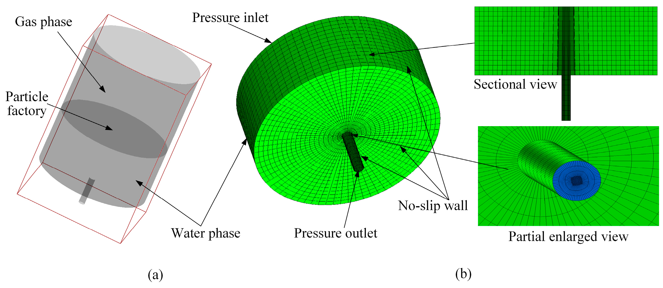
3.1. Calculation Model

To reveal motion laws of the flow field under the comprehensive action of Coriolis acceleration and initial prerotation disturbance, the mixing flow pumping model is presented to perform numerical simulation, as shown in Figure 1. Aiming at the flow of particle phase in the flow field, a three-dimensional cylindrical container geometric model should be introduced under the solution framework of EDEM 2.7 software. A particle factory is set up at the gas–liquid–solid interface to generate many randomly distributed particles, which have no initial velocity and are only affected by gravity. Grid division is a cylindrical container model with finite space treated by discretization, and its partition size is directly related to the time and accuracy of numerical calculation. A high-quality grid division with an appropriate scale can improve the convergence of model calculation, numerical accuracy, and calculation efficiency. Hexahedral structured mesh has high mesh quality, low numerical diffusion, and high precision and is suitable for meshing the numerical model in this section. First, the Cooper algorithm encrypts the center area of the large cylinder and the drainage pipe. Then, the standard hexahedral multi-block structured grid is used to mesh the remaining fluid domain, and the number of grids is 467,126. As can be seen from the figure, the grid division of the model is relatively uniform, and the grid near the drainage pipe is relatively dense. The high-quality grid can ensure the accuracy requirements of numerical calculation.

3.2. Boundary Conditions

The formation processes of the three-phase mixing flows are observed in finite physical spaces. The vessel inlet is the pressure inlet, the vessel outlet denotes the pressure outlet, and container walls are defined as no-slip walls. A custom segmentation method separates the water and gas phases from the whole numerical model. The boundary conditions of the model are shown in Table 1. Initial speeds are applied to the entire region of the flow field. Four groups of tangential velocities (v = 1.5π, 2.0π, 2.5π, 3.0π rad/s) are selected for calculation.
The finite volume method should be considered to solve control equations to ensure the strict conservation of fluid mass. Due to mixing flow simulation being a typical transition flow calculation and the multiphase changes being nonlinear, the pressure and velocity coupling processing adopts the pressure implicitly with the splitting of the operator algorithm to satisfy converged efficiencies [44,45,46]. The CFD-DEM coupling method is performed via user-defined functions (UDFs). The pressure staggering option (PRESTO) is adopted to address staggering internal pressure changes and higher rotating flows [47,48]. The physical parameters are listed in Table 2.

3.3. Grid Independence Study

The primary sources of error between numerical calculation and experimental value are model approximation error, difference equation stage error, discretization/iteration/rounding error of solving region, etc. In the calculation process, the discrete error decreases with the thinning of the grid. However, as the number of discrete points increases with the thinning of the grid, the rounding error also increases [49,50]. In engineering fluid calculation, how grids are generated in irregular regions has an essential influence on the calculation results and efficiency. Therefore, in this paper, the structured grid-quadrilateral mesh is adopted for grid division, and the grid qualities are better to accord with the precision and repeatability of calculation results.
In Figure 2, the turbulence energies of different grid numbers show similar trends. When the number of grids reaches a specific value, the turbulent kinetic energy curve shows an almost uniform distribution. Low grid resolution has some errors near the wall surface and cannot obtain accurate results. However, grid resolution (N = 467,126 and N = 594,073) can meet the requirements of grid independence, and the numerical error is less than 5%.

4. Results and Discussion

4.1. Transport Dynamic Characteristics of Mixing Flows

According to the calculation model, the formation process of multiphase mixing flows is studied, the fluid interface can be tracked in real time, and the critical formation mechanism is revealed. Pumping refers to the phenomenon of the fluid phase in contact with the surface medium being drawn away by the drain and mixed with the lower liquid in the process of liquid-free drain convergence, which is called the pumping phenomenon. During the mixing flow formation process, the morphology evolution of the interface has nonlinear characteristics due to the suction force changes. The volume fraction profile reflects the evolution laws of interphase interfaces, as shown in Figure 3.
In the early stage of mixing flow formation, the flow pattern of the fluid is manifested as axial motion and tangential motion (Figure 3a–d). With the drop of the free surface, the surface center is concave towards the direction of the outlet, and the surface height is lower than that at both ends, indicating that the mixing flow is formed. The initial tangential speeds raise the Reynolds number, enhancing the tangential motion and increasing the flow convergence rate moving from walls to centers. Here, the initial disturbance factor controls the entire flow field motion and is balanced with viscous forces, gravity, and wall resistance. As liquid levels drop, strong suction is generated in the center of the two-phase interface, and a significant amount of gas is sucked into the pipe outlet, as shown in Figure 3e. Intense pumping action can overcome fluid viscous resistances.
As the inspiratory stage develops and matures, many upper gases are continuously pumped to the lower liquid level and rapidly accumulate to form large bubbles to exit the water outlet. It is the extraction stage, as shown in Figure 3f,g. The suction stage maintains the V-shaped opening size of the suction stage, and the suction hole, namely the lowest liquid level, is just flush with the bottom of the barrel. When the gas columns are formed, the flow speeds of the two-phase are zero, indicating that the mixing flow reaches the penetration state (Figure 3h,i). The above flow characteristic is in accord with the numerical results by Tan et al. [51]. However, their research cannot observe the clear suction port. The critical suction formation course is the crucial state of fluid transitions, which is significant to some industrial applications.
The streamlined distribution diagrams are given to analyze the mixing flow pumping process, as shown in Figure 4. The flow line trend and air and water distribution are generally the same in the formation course. At the top part of the drain hole, very little air in the center is sucked into the water outlet through the suction hole, and most of the air flows back along the liquid level tangentially, as shown in Figure 4b,c. Local reflux vortices are formed near the center line. The above characteristics are in accord with the experiment results of Andersen et al. [52,53]. This predicted result is also in accordance with the visualization experiment results by Chen et al. [54], who found that a two-celled structure exists owing to the Ekman layer. From the above-mentioned phenomena, it can be concluded that the macroscopic motions of mixing flows lead to highly higher turbulence mass, momentum, and energy transport efficiency.
The evolution curve of the air-phase volume fraction corresponding to each stage is shown in Figure 5. The volume fraction gradually vibrates violently after 28 s. During mixing flow suction, air bubbles form underwater and drain out of the water outlet. The farther the amplitude from the horizontal axis, the larger the volume of the expelled bubble. The above phenomena indicate that energy is concentrated in the range of low wave number vortices for turbulent flow, while dissipation occurs in higher-wavenumber vortices. Hence, the energy transport course from large-scale vortices to small-scale vortices exists.
The mixing flow characteristic is shown in Figure 6. The dynamic pressure is directly related to the rotational speed, as shown in Figure 6a. In the drainage stage, the rotational speed remains unchanged, so the total pressure in the process presents a similar trend. Figure 6b shows the cloud diagram of radial velocity corresponding to the mixing flow. The velocity is more significant in the suction stage. The free surface of the mixing flow has variable speed gradients in radial directions. The cloud diagram of the turbulent energy is shown in Figure 6c. The turbulence energy has an enormous value at the drainage, as shown in Figure 6c. Above the pipe port, the section’s turbulent kinetic energy near the port is the largest due to the large flow velocity, and a strong suction phenomenon is formed. The above phenomenon shows that the potential energy reaches the largest values at the suction stage, and there is a concentrated release in the extraction stage. There is a conversion mechanism of kinetic energy and potential energy. Figure 6d shows the total pressure characteristics of the mixing course. The pressure takes on uniform distribution characteristics, and the vortex center has a lower pressure value.
Based on the above cloud diagrams, the following mixing characteristic curves are obtained (Figure 7). In Figure 7a, the velocity value between z = 0.18 m and z = −0.22 m is negative, indicating liquid velocity. A greater velocity value can be found near the nozzle. Curve z = 0.24 m represents gas-phase velocity. Finally, the four curves tend to zero, indicating that disturbance, inertia forces, and viscous resistance forces in the whole system maintain a balance, the water flow does not tend to flow toward the wall, and the surface opening remains constant. It shows that the vortices are formed and satisfy the kinematic properties of Rankin-like vortices. The dynamic pressure increases with the increase in radial coordinates in Figure 7b. This is because the high rotational speed near the wall leads to the increase in dynamic pressure value. In the mixing flow center, the dynamic pressure values of different sections vary slightly, which is caused by the gas–liquid–solid coupling disturbance. In Figure 7c, the turbulent energy takes on uniform trends and has no apparent difference. The wall has the largest value due to the swirling effect. In Figure 7d, the pressure at the same x coordinate in each period is the same. The static pressure accounts for a more significant proportion of the total pressures relative to the dynamic pressures. In the full discharge stage, the rotational speed is unchanged, so the total pressure in the process presents roughly the same trend.

4.2. Effect of the Initial Swirling Intensity on the Critical Pumping State

As the vortices reach the pumping state, the surface fluids can be pumped into the drain hole. The impurity flows along the mixing flow surfaces to pipes and affects industrial production. Therefore, the critical suction state is selected to investigate the influences of the initial speeds on the flow field (Figure 8).
When the initial speed rises, the height of the liquid surfaces rises. As the turbulence intensity rises, the centrifugal force of the fluid increases rapidly, which enhances the tendency of the liquid phase to flow to the wall surface. When the disturbance speed increases, the opening angles of the liquid surfaces are smaller in the mixing flow critical state. The macroscopic motions of mixing flows enhance the higher transport efficiencies of turbulence mass and momentum, accelerate the suction courses of the vortices, and make the vortices penetrate the exhaust tube quickly.
Based on the above, the relationship between the rotational component and the phase of mixing flow suction is studied. Figure 9 describes the radial speed curve of the fluid field average developing into the inspiratory stage at a particular time at different rotational speeds. In Figure 9a, radial velocities under different initial perturbations show the same evolution trend at the section curve z = 0.18 m. The radial velocity values differ slightly at the intersection of gas–liquid–solid mixing flows. Figure 9b shows the radial velocity curve of the gas phase. Radial distribution of velocities differs significantly under different initial disturbance velocities. This is due to the V-shaped opening shape of the mixing flow. However, it can be seen that as the mixing flow arrives at the pumping state, the disturbance factors of flow fields are in dynamic equilibrium with the inertial forces and viscous resistances. There is no tendency for the fluid to flow toward the walls, and the opening scales remain constant.

4.3. Particle Flow Patterns

To explore the particle flow modes, particle distribution diagrams are obtained (Figure 10). The particle factory generates the desired particle phase in the initial flow state, and the initial disturbance speed has minimal effects on the particle phase. Still, the particles show apparent circular motion. In Figure 10a, particles are formed at the cross-section and suspended on the liquid surface with random distribution characteristics. The central regions of liquid surfaces sink rapidly due to gravity and the velocity of the initial disturbance. In Figure 10b, the initial rotation speeds can offer specific circumferential energy, causing the fluid and particles on the walls to move upward. The free liquid dents move the granular fluid in axial and radial directions (Figure 10c). As the mixing flows evolve, the particle numbers in the center rise significantly, increasing particle concentration and particle heights near the walls. In Figure 10d, particles in the bottom area are sucked into pipe holes under the mixing flow. These phenomena indicate that the mixing of flow-pumping particles consumes much turbulent energy and decreases turbulence energy.
The streamlined evolution process of particles is obtained to explore the flow trajectory of particles, as shown in Figure 11. Under initial disturbance degree and gravity, the particles in the center move towards the water mouth under the force in the vertical direction. The particles near the wall move upward as the liquid surface floats up under the action of rotation velocity in Figure 11a,b. As the mixing flow evolves, the central particles accumulate, and the volume fraction reaches the maximum in the inspiratory stage. At this time, some particles are transported by strong suction at the water outlet, as shown in Figure 11c. The maximum particle speed near the mouth is 2.75 m/s. When some particles are pumped, the turbulence energy dissipates, which induces a decrease in the energy and a decrease in the speed value of some particles, as shown in Figure 11d. The particles in the central region flow faster under axial suction. The particles near the water surface rotate under the action of disturbance velocity, forming a ring flow pattern. The particle flow is in a relative equilibrium under centrifugal and radial forces. The above phenomena show that the particles in the center of the mixing flow have high randomness and are nonlinear under the intense suction action of the nozzle. The aggregation and dissipation of turbulence energy lead to the weakening of the particle suction effect.
According to the above particle results, the particle velocity and force characteristics in the transport process are obtained, as shown in Figure 12. In the transport process, particles are transported axially from the free surface under the outlet suction actions. In Figure 12a, the particles have a smaller velocity in the initial phase. When the mixing flow develops, the velocity of the particles increases, and they are in a state of dynamic equilibrium for a specific time. In the later stage of drainage, the velocity of the particles increases instantaneously due to the suction force of the water nozzle, and the peak velocity is 3.30 m/s. When the particles are transported, the velocity of the particles decreases instantly. Figure 12b describes the characteristics of particle force evolution. It can be seen that in the early and middle stages, the force of the particles is constant. At this time, the particles can be influenced by centrifugal force and gravity. However, when the particles move along the axial direction, the suction effect of the water nozzle increases, resulting in the rapid increase in the force of the particles, and the peak value of the force is 0.0078 N. The above phenomenon shows that the flow pattern evolution of particles is mainly affected by the suction force of the water inlet. Improving the design of the nozzle and reducing its suction force can avoid the impurities transported by swirl suction, which has important guiding significance for the chemical extraction process.
To obtain particle energy evolution laws, the dynamic force energy characteristics of particles in the transport process are obtained, as shown in Figure 13. In Figure 13a, the particles have smaller turbulence energy during the initial and middle evolution of the swirl flow. At t = 20 s, affected by the suction of the water nozzle, the particle energy rises, and the peak value is 0.27 × 10⁻³ m2·s−2. In Figure 13b, particles have the maximum potential energy in the initial evolution course. At this time, particles are in a higher position, and the peak potential energy is 0.155 m2·s−2. With the evolution of the mixing field, the potential energy of particles decreases, and there is an energy transition process when the kinetic energy is at its maximum and particle potential energy is small. In Figure 13c, the total energy of particles suddenly increases when t = 3 s. The total energy is dominated by potential energy. With the development of the mixing field, the total energy decreases to between t = 3 s and t = 20 s, which is consistent with the potential energy characteristics of Figure 13b. At t = 20 s, the total energy is mainly dominated by kinetic energy, resulting in a significant increase in the total energy. Subsequently, the total energy is dissipated during the swirl transport process. The above process shows the particle pumping course’s dynamic energy transformation mechanism.

5. Conclusions

Investigating the material mass transfer characteristic and disturbance regulation strategy of multiphase flows has important scientific values and industrial prospects. This paper put forward a modeling approach oriented on gas–liquid–solid mixing flows to study the material mass transfer mechanism and compare the evolution characteristics of flow fields under dynamic disturbance regulation.
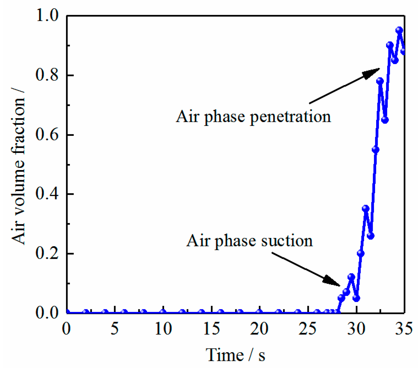
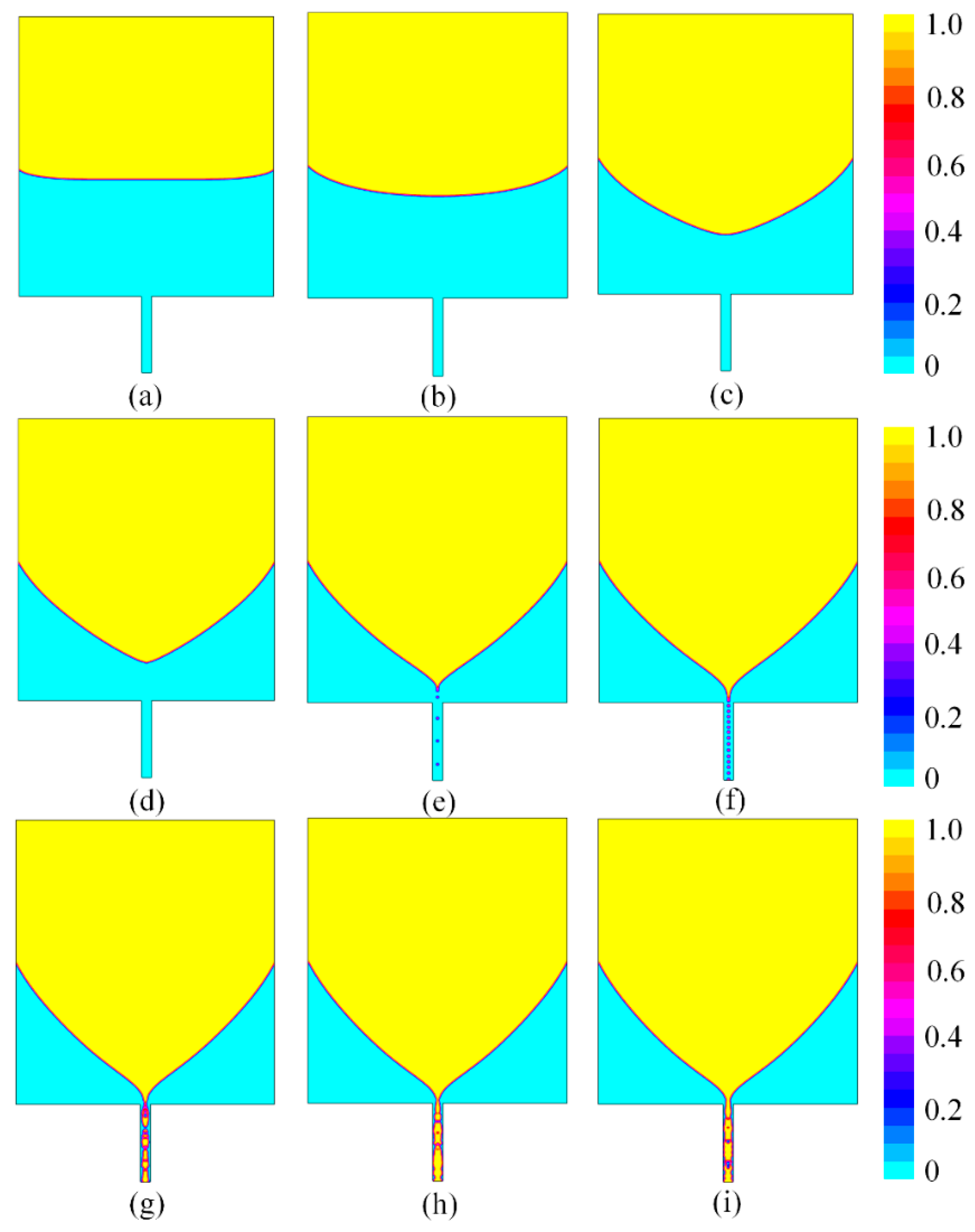
  • Based on the CFD-DEM coupling method and particle porous model, a three-phase mixing flow mass transfer model is put forward to obtain the distribution of relevant physical variables (volume fraction, velocity, and streamline). The critical formation time denotes the crucial transition state of fluid mediums. The fluid composition transition affects quality and production efficiency in the metallurgy, chemical industry, and other industrial processes.
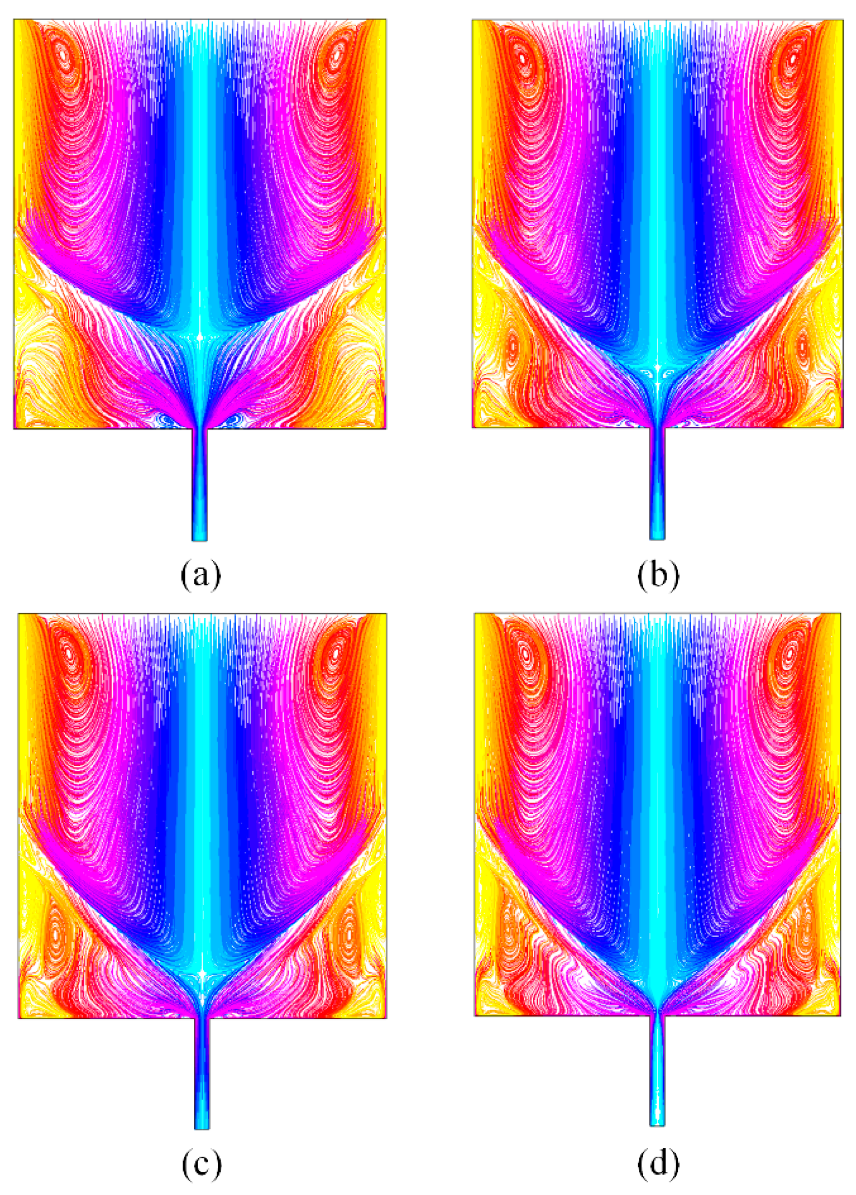
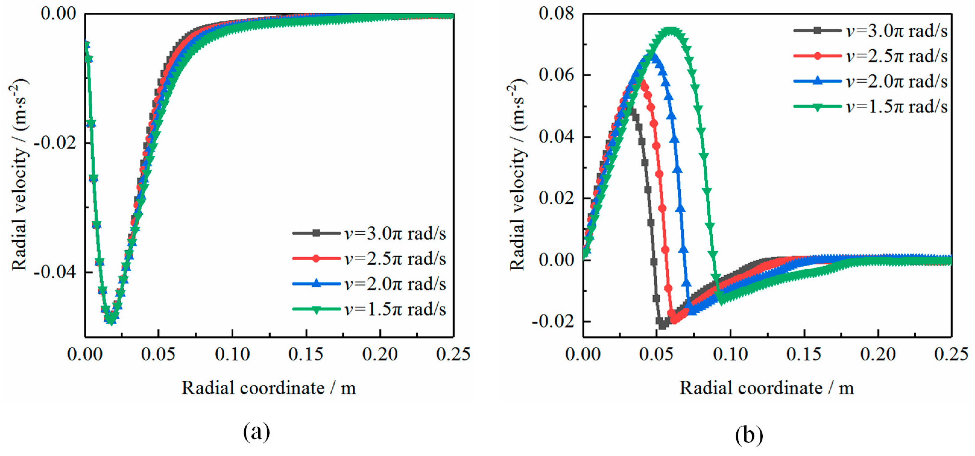
  • Initial disturbance speeds are the critical factor of mixing pumping formation. Under the influence of initial disturbance, the fluid microcluster on the surfaces has different disturbance patterns, inducing different speed gradients. As the mixing flow reaches the inspiratory state, the disturbance factors are in equilibrium with the inertia forces and viscous resistance. The macroscopic motions of mixing flows enhance higher transfer efficiencies of mass, momentum, and energy and make vortices penetrate the drain pipe.
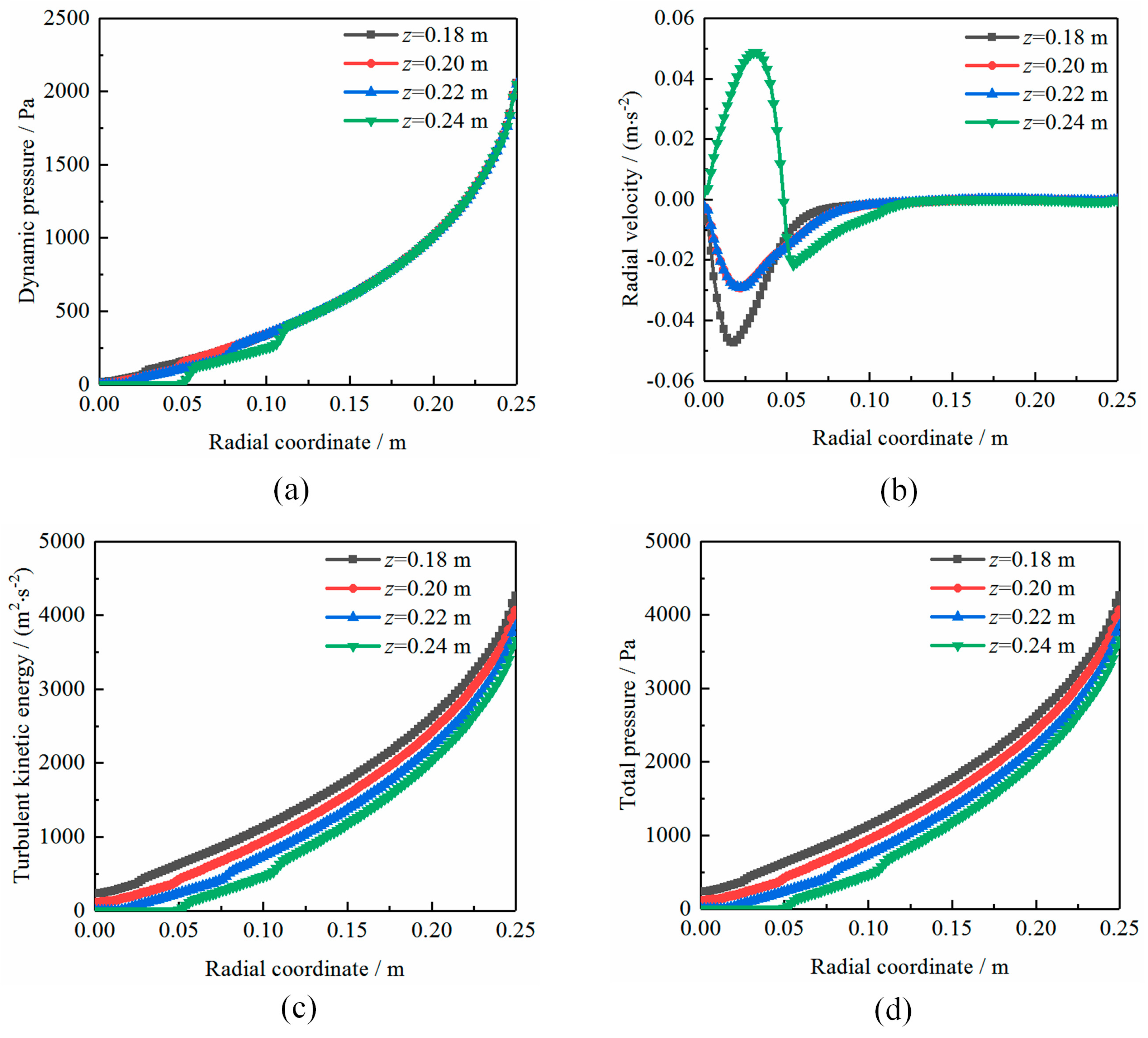
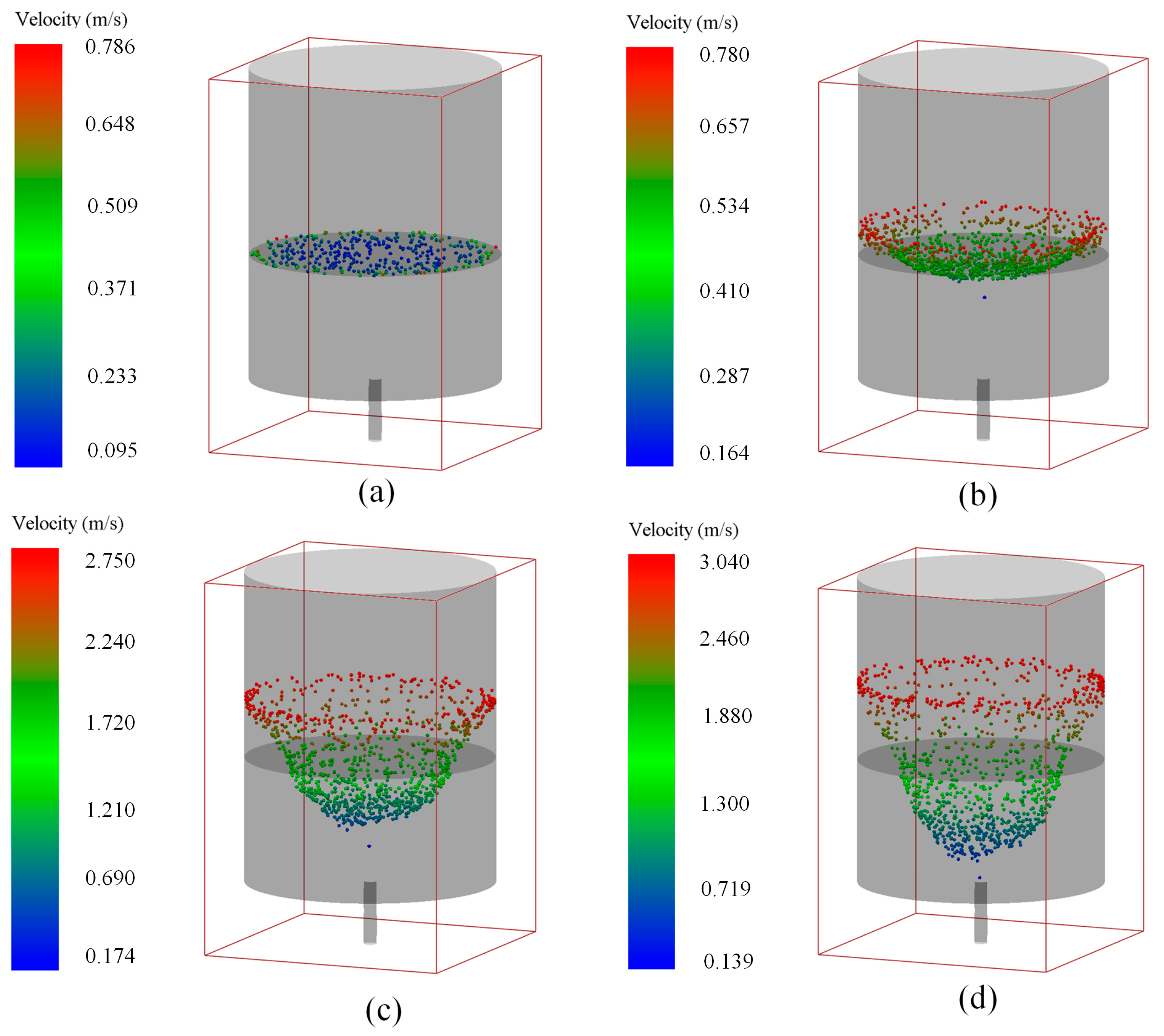
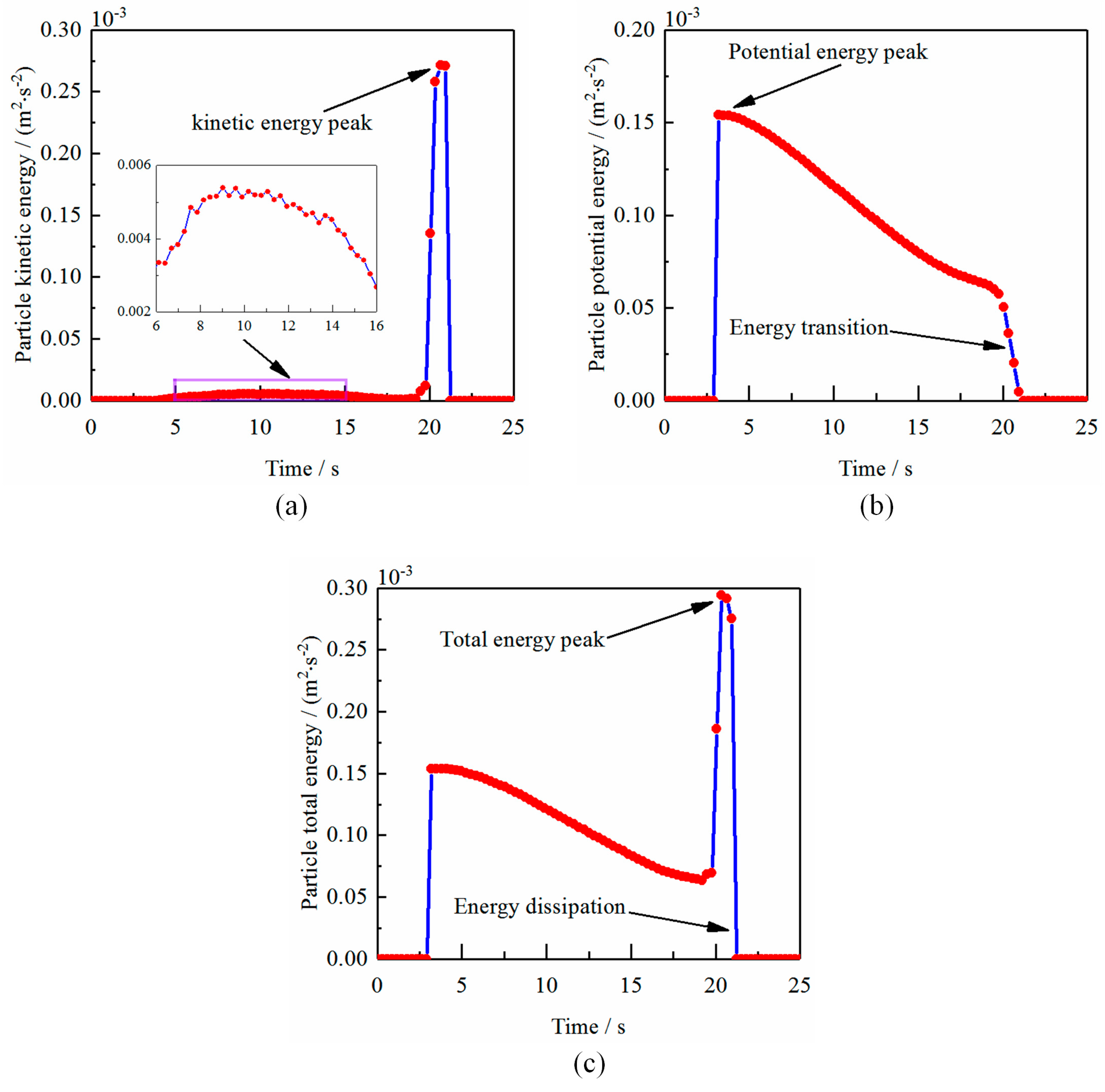
  • The particles in the mixing flow center have high randomness and nonlinearity under the intense suction action of the water nozzle. The aggregation and dissipation of turbulence energies lead to the weakening of particle pumping effects. The suction of the water inlet can influence the flow pattern evolution of particles in the mixing course, and the particle’s total energy is dissipated during the swirl transport process.

Author Contributions

Conceptualization, X.F. and Q.Y.; article identification, screening, retrieval, selection, and analysis, Q.Y. and L.L.; writing—original draft preparation, Q.Y. and L.L.; funding acquisition, Q.Y. and L.L.; tables and figures generation, Q.Y., G.Z. and X.F.; review and editing, Q.Y.; formal analysis and investigation, Q.Y.; supervision, Q.Y. All authors have read and agreed to the published version of the manuscript.

Funding

This work was partly supported by the Zhejiang Soft Science Research Program Project (2024C35116); National and Regional Research Project on German Speaking Countries of Zhejiang University of Science and Technology (2023DEGB009); Fundamental Research Funds for the Provincial Universities of Zhejiang University of Science and Technology under Grant No. 2023QN041; Zhejiang Provincial Natural Science Foundation under Grant No. LQ23E050017.

Institutional Review Board Statement

Not applicable.

Informed Consent Statement

Not applicable.

Conflicts of Interest

The authors declare no conflict of interest.

References

  1. Chen, J.C.; Han, P.C.; Zhang, Y.; You, T.; Zheng, P.Y. Scheduling energy consumption-constrained workflows in heterogeneous multi-processor embedded systems. J. Syst. Archit. 2023, 142, 102938. [Google Scholar] [CrossRef]
  2. Zheng, G.A.; Gu, Z.H.; Xu, W.X.; Li, Q.H.; Tan, Y.F.; Wang, C.Y.; Li, L. Gravitational surface vortex formation and suppression control: A review from hydrodynamic characteristics. Processes 2023, 11, 42. [Google Scholar] [CrossRef]
  3. Chen, J.T.; Ge, M.; Li, L.; Zheng, G. Material transport and flow pattern characteristics of gas–liquid–solid mixed flows. Processes 2023, 11, 2254. [Google Scholar] [CrossRef]
  4. Jin, Z.; He, D.; Wei, Z. Intelligent fault diagnosis of train axle box bearing based on parameter optimization VMD and improved DBN. Eng. Appl. Artif. Intell. 2022, 110, 104713. [Google Scholar] [CrossRef]
  5. Conzalez, J.F.; Sanson, L.Z. Linear stability of monopolar vortices over isolated topography. J. Fluid Mech. 2023, 959, A23. [Google Scholar] [CrossRef]
  6. Wei, Z.X.; He, D.Q.; Jin, Z.Z.; Liu, B.; Shan, S.; Chen, Y.J.; Miao, J. Density-based affinity propagation tensor clustering for intelligent fault diagnosis of train bogie bearing. IEEE Trans. Intell. Transp. Syst. 2023, 24, 6053–6064. [Google Scholar] [CrossRef]
  7. Li, L.; Li, Q.H.; Ni, Y.S.; Wang, C.Y.; Tan, Y.F.; Tan, D.P. Critical penetrating vibration evolution behaviors of the gas-liquid coupled vortex flow. Energy 2023, in press. [Google Scholar]
  8. Liu, Y.; Li, P.; Wang, Y.; Guo, H.Y.; Zhang, X.T. Experimental investigation on the vortex-induced vibration of the vertical riser fitted with the water jetting active vibration suppression device. Int. J. Mech. Sci. 2020, 177, 105600. [Google Scholar] [CrossRef]
  9. Li, H.X.; Wang, Q.; Lei, H. Mechanism analysis of free-surface vortex formation during steel Teeming. ISIJ Int. 2014, 54, 1592–1600. [Google Scholar] [CrossRef]
  10. Li, L.; Tan, Y.F.; Xu, W.X.; Ni, Y.S.; Yang, J.G.; Tan, D.P. Fluid-induced transport dynamics and vibration patterns of multiphase vortex in the critical transition states. Int. J. Mech. Sci. 2023, 252, 108376. [Google Scholar] [CrossRef]
  11. Su, R.A.; Gao, Z.Y.; Chen, Y.Y.; Zhang, C.Q. Large-eddy simulation of the influence of hairpin vortex on pressure coefficient of an operating horizontal axis wind turbine. Energy Convers. Manag. 2022, 267, 115864. [Google Scholar] [CrossRef]
  12. Romero, A.; Tadeu, A.; Galvín, P. 2.5D coupled BEM–FEM used to model fluid and solid scattering wave. Int. J. Numer. Methods Eng. 2015, 101, 148–164. [Google Scholar] [CrossRef]
  13. Zhao, Y.Z.; Gu, Z.L.; Yu, Y.Z.; Li, Y.; Feng, X. Numerical analysis of structure and evolution of free water vortex. J. Xi’an Jiaotong Univ. 2003, 37, 85–88. [Google Scholar]
  14. Mazzaferro, G.M.; Piva, M.; Ferro, S.P. Experimental and numerical analysis of ladle teeming process. Ironmak. Steelmak. 2004, 31, 503–508. [Google Scholar] [CrossRef]
  15. Xie, H.Y.; Cao, Y.; Qin, F.H.; Luo, X.S. The slip effect of micro-droplets in Rankine vortex. Sci. Sin. Phys. Mech. Astron. 2017, 47, 124702-1–124702-9. [Google Scholar] [CrossRef]
  16. Tang, H.Y.; Liang, Y.C. Formation mechanism and influence factors of sink vortex during ladle teeming. Acta Metall. Sin. 2015, 52, 519–528. [Google Scholar]
  17. Afra, B.; Karimnejad, S.; Delouei, A.A.; Tarokh, A. Flow control of two tandem cylinders by a highly flexible filament: Lattice spring IB-LBM. Ocean Eng. 2022, 250, 111025. [Google Scholar] [CrossRef]
  18. Delouei, A.A.; Karimnejad, S.; He, F.L. Direct Numerical Simulation of pulsating flow effect on the distribution of non-circular particles with increased levels of complexity: IB-LBM. Comput. Math. Appl. 2022, 121, 115–130. [Google Scholar] [CrossRef]
  19. Che, H.Q.; Werner, D.; Seville, J. Evaluation of coarse-grained CFD-DEM models with the validation of PEPT measurement. Particuology 2023, 82, 48–63. [Google Scholar] [CrossRef]
  20. Qu, Z.G.; Jin, S.; Wu, L.Q.; An, Y.; Liu, Y.; Fang, R.; Tang, J. Influence of water flow velocity on fouling removal for pipeline based on eco-friendly ultrasonic guided wave technology. J. Clean. Prod. 2019, 240, 118173. [Google Scholar] [CrossRef]
  21. Chashechkin, Y.D. Transfer of the Substance of a Colored Drop in a Liquid Layer with Travelling Plane Gravity-Capillary Waves. Izv. Atmos. Ocean. Phys. 2022, 58, 188–197. [Google Scholar] [CrossRef]
  22. Zheng, G.A.; Shi, J.L.; Li, L.; Li, Q.H.; Gu, Z.H.; Xu, W.X.; Lu, B. Fluid-solid coupling-based vibration generation mechanism of the multiphase vortex. Processes 2023, 11, 568. [Google Scholar] [CrossRef]
  23. Isherwood, L.; Grant, Z.J.; Cottlieb, S. Strong stability preserving integrating factor two-step Runge-Kutta methods. J. Sci. Comput. 2019, 81, 1446–1471. [Google Scholar] [CrossRef]
  24. Li, L.; Yang, Y.S.; Xu, W.X.; Lu, B.; Gu, Z.H.; Yang, J.G.; Tan, D.P. Advances in the multiphase vortex-induced vibration detection method and its vital technology for sustainable industrial production. Appl. Sci. 2022, 12, 8538. [Google Scholar] [CrossRef]
  25. Li, C.J.; Zou, Y.Q.; Li, G.Y. Hydrodynamic characteristics of pyrolyzing biomass particles in a multi-chamber fluidized bed. Powder Technol. 2023, 421, 118403. [Google Scholar] [CrossRef]
  26. Tan, Y.F.; Ni, Y.S.; Wu, J.F.; Li, L.; Tan, D.P. Machinability evolution of gas-liquid-solid three-phase rotary abrasive flow finishing. Int. J. Adv. Manuf. Technol. 2023, in press. [Google Scholar] [CrossRef]
  27. Li, L.; Qi, H.; Yin, Z.C.; Li, D.F.; Zhu, Z.L.; Tangwarodomnukun, V.; Tan, D.P. Investigation on the multiphase sink vortex Ekman pumping effects by CFD-DEM coupling method. Powder Technol. 2020, 360, 462–480. [Google Scholar] [CrossRef]
  28. Wang, T.; Li, L.; Yin, Z.C.; Xie, Z.W.; Wu, J.F.; Zhang, Y.C.; Tan, D.P. Investigation on the flow field regulation characteristics of the right-angled channel by impinging disturbance method. Proc. Inst. Mech. Eng. Part C J. Mech. Eng. Sci. 2022, 236, 11196–11210. [Google Scholar] [CrossRef]
  29. Shen, J.H.; Jin, C.L.; Yuan, J.M. Experimental and numerical analysis of hopper dust suppression during discharge of free falling bulk solids. Powder Technol. 2023, 415, 118108. [Google Scholar] [CrossRef]
  30. Lin, L.; Tan, D.P.; Yin, Z.C.; Wang, T.; Fan, X.H.; Wang, R.H. Investigation on the multiphase vortex and its fluid-solid vibration characters for sustainability production. Renew. Energy 2021, 175, 887–909. [Google Scholar]
  31. Tan, Y.F.; Ni, Y.S.; Xu, W.X.; Xie, Y.S.; Li, L.; Tan, D.P. Key technologies and development trends of the soft abrasive flow finishing method. J. Zhejiang Univ.-Sci. A 2023, in press. [Google Scholar] [CrossRef]
  32. Chen, J.C.; Li, T.Y.; You, T. Global-and-Local Attention-Based Reinforcement Learning for Cooperative Behaviour Control of Multiple UAVs. IEEE Trans. Vehicular Technol. 2023, in press. [Google Scholar] [CrossRef]
  33. Tashakori-Asfestani, F. Effect of inter-particle forces on solids mixing in fluidized beds. Powder Technol. 2023, 415, 118098. [Google Scholar] [CrossRef]
  34. Li, L.; Tan, D.P.; Wang, T.; Yin, Z.C.; Fan, X.H.; Wang, R.H. Multiphase coupling mechanism of free surface vortex and the vibration-based sensing method. Energy 2021, 216, 119136. [Google Scholar] [CrossRef]
  35. Yu, J.H.; Wang, S.; Kong, D.L. Coal-fueled chemical looping gasification: A CFD-DEM study. Fuel 2023, 345, 128119. [Google Scholar] [CrossRef]
  36. Zhang, L.; Wang, J.S.; Tan, D.P.; Yuan, Z.M. Gas compensation-based abrasive flow processing method for complex titanium alloy surfaces. Int. J. Adv. Manuf. Technol. 2017, 92, 3385–3397. [Google Scholar] [CrossRef]
  37. Li, L.; Lu, J.F.; Fang, H.; Yin, Z.C.; Wang, T.; Wang, R.H.; Fan, X.H.; Zhao, L.J.; Tan, D.P.; Wan, Y.H. Lattice Boltzmann method for fluid-thermal systems: Status, hotspots, trends and outlook. IEEE Access 2020, 8, 27649–27675. [Google Scholar] [CrossRef]
  38. Wang, X.Y.; Gong, L.; Li, Y.; Yao, J. Developments and applications of the CFD-DEM method in particle-fluid numerical simulation in petroleum engineering: A review. Appl. Therm. Eng. 2022, 222, 119865. [Google Scholar] [CrossRef]
  39. Li, L.; Gu, Z.H.; Xu, W.X.; Tan, Y.F.; Fan, X.H.; Tan, D.P. Mixing mass transfer mechanism and dynamic control of gas-liquid-solid multiphase flow based on VOF-DEM coupling. Energy 2023, 272, 127015. [Google Scholar] [CrossRef]
  40. Wang, J.; Ku, X.K. Numerical simulation of biomass steam gasification in an internally interconnected fluidized bed using a two-grid MP-PIC model. Chem. Eng. Sci. 2023, 272, 119608. [Google Scholar] [CrossRef]
  41. Yin, Z.C.; Lu, J.F.; Li, L.; Wang, T.; Wang, R.H.; Fan, X.H.; Lin, H.K.; Huang, Y.S.; Tan, D.P. Optimized Scheme for Accelerating the Slagging Reaction and Slag-Metal-Gas Emulsification in a Basic Oxygen Furnace. Appl. Sci. 2020, 10, 5101. [Google Scholar] [CrossRef]
  42. Zhu, X.L.; Liu, Y.B. Bubble behaviors of geldart B particle in a pseudo two-dimensional pressurized fluidized bed. Particuology 2023, 79, 121–132. [Google Scholar] [CrossRef]
  43. Wang, S.; Shen, Y.S. CFD-DEM-VOF-phase diagram modelling of multi-phase flow with phase changes. Chem. Eng. Sci. 2023, 273, 118652. [Google Scholar] [CrossRef]
  44. Li, L.; Lu, B.; Xu, W.X.; Gu, Z.H.; Yang, Y.S.; Tan, D.P. Mechanism of multiphase coupling transport evolution of free sink vortex. Acta Phys. Sin. 2023, 72, 034702. [Google Scholar] [CrossRef]
  45. Liu, L.; Zhang, X.T.; Tian, X.L.; Li, X. Numerical investigation on dynamic performance of vertical hydraulic transport in deepsea mining. Appl. Ocean Res. 2023, 130, 103443. [Google Scholar] [CrossRef]
  46. Li, L.; Xu, W.X.; Tan, Y.F.; Yang, Y.S.; Yang, J.G.; Tan, D.P. Fluid-induced vibration evolution mechanism of multiphase free sink vortex and the multi-source vibration sensing method. Mech. Syst. Signal Process. 2023, 189, 110058. [Google Scholar] [CrossRef]
  47. Tan, D.P.; Li, L.; Li, D.F.; Zhu, Y.L.; Zheng, S. Ekman boundary layer mass transfer mechanism of free sink vortex. Int. J. Heat Mass Transf. 2020, 150, 119250. [Google Scholar] [CrossRef]
  48. Sun, Z.; Jin, H.; Xu, Y. Severity-insensitive fault diagnosis method for heat pump systems based on improved benchmark model and data scaling strategy. Energy Build. 2022, 256, 111733. [Google Scholar] [CrossRef]
  49. Lu, J.F.; Wang, T.; Li, L.; Yin, Z.C. Dynamic Characteristics and Wall Effects of Bubble Bursting in Gas-Liquid-Solid Three-Phase Particle Flow. Processes 2020, 8, 760. [Google Scholar] [CrossRef]
  50. Tamburini, A.; Cipollina, A.; Micale, G. CFD simulations of dense solid-liquid suspensions in baffled stirred tanks: Prediction of the minimum impeller speed for complete suspension. Chem. Eng. J. 2012, 193, 234–255. [Google Scholar] [CrossRef]
  51. Tan, D.P.; Ni, Y.S.; Zhang, L.B. Two-phase sink vortex suction mechanism and penetration dynamic characteristics in ladle teeming process. J. Iron Steel Res. Int. 2017, 24, 669–677. [Google Scholar] [CrossRef]
  52. Andersen, A.; Bohr, T.; Stenum, B. Anatomy of a bathtub vortex. Phys. Rev. Lett. 2003, 91, 104502. [Google Scholar] [CrossRef]
  53. Andersen, A.; Bohr, T.; Stenum, B. The bathtub vortex in a rotating container. J. Fluid Mech. 2006, 556, 121–146. [Google Scholar] [CrossRef]
  54. Wu, J.F.; Li, L.; Li, Z.; Wang, T.; Tan, Y.F.; Tan, D.P. Mass transfer mechanism of multiphase shear flows and interphase optimization solving method. Energy 2023, in press. [Google Scholar]
Figure 1. Objective model and boundary conditions. (a) Physical model. (b) Numerical model and boundary condition.
Jmse 12 00084 g001
Figure 2. Grid independence research of the numerical model.
Jmse 12 00084 g002
Figure 3. Volume fraction cloud diagram of the gas phase (v = 3.0π rad/s). (a) t = 5.0 s. (b) t = 10.0 s. (c) t = 20.1 s. (d) t = 26.6 s. (e) t = 29.1 s. (f) t = 30.2 s. (g) t = 31.4 s. (h) t = 32.2 s. (i) t = 33.3 s.
Jmse 12 00084 g003
Figure 4. Streamline distribution diagrams. (a) t = 26.6 s. (b) t = 29.1 s. (c) t = 30.2 s. (d) t = 31.4 s.
Jmse 12 00084 g004
Figure 5. Variation curve of gas phase volume fraction.
Jmse 12 00084 g005
Figure 6. Characteristic diagrams of the mixing flow field. (a) Dynamic pressure. (b) Radial velocity. (c) Turbulent energy. (d) Total pressure.
Jmse 12 00084 g006
Figure 7. Characteristic curves of the mixing flow field. (a) Dynamic pressure. (b) Radial velocity. (c) Turbulent energy. (d) Total pressure.
Jmse 12 00084 g007
Figure 8. Volume fraction cloud diagrams of the gas phase in the pumping state. (a) t = 49.2 s. (b) t = 53.7 s. (c) t = 60.9 s. (d) t = 40.0 s. (e) t = 45.1 s. (f) t = 49.6 s. (g) t = 33.0 s. (h) t = 37.1 s. (i) t = 43.0 s.
Jmse 12 00084 g008
Figure 9. Radial velocity curves of vortices under different initial disturbances. (a) z = 0.18 m. (b) z = 0.24 m.
Jmse 12 00084 g009
Figure 10. Particle flow patterns under initial disturbances. (a) t = 0.0 s. (b) t = 5.0 s. (c) t = 15.0 s. (d) t = 20.6 s.
Jmse 12 00084 g010
Figure 11. Particle flow patterns under the initial disturbances. (a) t = 1.0 s. (b) t = 5.0 s. (c) t = 15.0 s. (d) t = 20.6s.
Jmse 12 00084 g011
Figure 12. Particle velocity and force at the pumping transport processes. (a) Particle velocity. (b) Particle force.
Jmse 12 00084 g012
Figure 13. Particle energy variation at the pumping transport processes. (a) Particle kinetic energy. (b) Particle potential energy. (c) Particle total energy.
Jmse 12 00084 g013
Table 1. Boundary conditions of the calculation model.
ItemParameter
InletPressure inlet
OutletPressure outlet
WallNo-slip wall
Gravity/(N)9.81
Pipeline length/(m)0.15
Pipeline diameter/(m)0.010
Gas phase elevation/(m)0.15
Water phase elevation/(m)0.40
Container elevation/(m)0.55
Container diameter/(m)0.5
Table 2. Physical parameters of the computations.
ParameterValue
Water density (kg/m3) 980
Gas density (kg/m3)1.225
Particle diameter (mm)20
Particle density (kg/m3) 950
Restitution coefficient, e0.9
Time step of CFD, (s)1.01 × 10⁻⁵
Time step of DEM, (s)2.36 × 10⁻⁷
Disclaimer/Publisher’s Note: The statements, opinions and data contained in all publications are solely those of the individual author(s) and contributor(s) and not of MDPI and/or the editor(s). MDPI and/or the editor(s) disclaim responsibility for any injury to people or property resulting from any ideas, methods, instructions or products referred to in the content.

