Metric Reliability Analysis of Autonomous Marine LiDAR Systems under Extreme Wind Loads

Abstract

As the key route detection device, the performance of marine LiDAR in harsh environments is of great importance. In this paper, a metric reliability analysis method for marine LiDAR systems under extreme wind loads is proposed. First, a static measurement accuracy evaluation model for the LiDAR system is proposed, targeting the problem that the LiDAR measurement tail reduces the measurement accuracy. Second, the distribution of extreme wind speeds in the Pacific Northwest is investigated, and a wind load probability model is developed. Finally, the impact of hull fluctuations on LiDAR measurement accuracy is analyzed by performing hull fluctuation simulations based on the wind load probability model, and the relationship curve between the metric reliability and measurement accuracy of marine LiDAR systems under extreme wind loads is addressed using the Monte-Carlo method. Experimental results show that the proposed LiDAR static measurement accuracy evaluation model can improve the measurement accuracy by more than 30%. Meanwhile, the solved curve of the LiDAR metric reliability versus the measurement allowable error indicates that the metric reliability can reach above 0.89 when the allowable error is 60 mm, which is instructive for the reliable measurement of marine LiDAR systems during ship navigation.

1. Introduction

Safety of autonomous vessel navigation is a top priority for the shipping industry. Autonomous vessels may face a variety of potential obstacles while at sea, such as other ships, reefs, and ice floes. LiDAR measurements play a crucial role in navigation safety assurance. Therefore, the metric reliability of marine LiDAR systems is key to achieve accurate monitoring of route obstacles [1,2,3].

In view of the important role and status of marine LiDAR systems in route obstacle monitoring, many related studies have been conducted, and marine LiDAR systems have been initially built to verify accuracy and reliability. Thomas Clunie et al. proposed a LiDAR-based marine target pose measurement algorithm that successfully measures the spatial position of multiple obstacle targets within 450 m. However, in harsh environmental conditions, the LiDAR calibration process is prone to errors, which reduces the target pose measurement capability [4]. Hyun-Taek Choi et al. [5] proposed a Radially Based Nearest Neighbors (RBNN) clustering method for space measurement to obtain the range, elevation, and azimuth angles of the marine targets. Leo Stanislas et al. [6] proposed a LiDAR-based marine target localization system and its calibration strategy for constructing 3D obstacle maps, which was validated in the Maritime RobotX Challenge and achieved spatial localization accuracy of 0.2 m. Andrzej Stateczny et al. [7] proposed a LiDAR-based detection method for coastal structures and obstacles, which effectively avoids collision problems during ship docking, with an average repeated measurement error of 1.19 m in the 100 m range. Jungwook Han et al. [8] proposed a LiDAR-equipped vehicle to improve autonomous navigation capability, which was able to achieve the location and trajectory of obstacle targets within 700 m, with an estimation error of nearly 20 m.

As can be seen from the current state of research, improving metric accuracy and reliability remains a focus for marine LiDAR systems [9,10], especially in harsh environmental conditions, as mentioned in [4]. Therefore, the effect of extreme wind loads on the metric reliability of marine LiDAR systems cannot be neglected. The following problems are faced during the research process. (1) Currently, most of the validation work on LiDAR systems is done in relatively smooth waters, however, the accuracy is not satisfactory, and the static metric accuracy of LiDARs still needs to be further optimized. (2) Due to the strong stochasticity of the wind fields, it is difficult to build realistic and comprehensive wind load models to provide load data for the analysis of hull roll and pitch characteristics. (3) Meanwhile, establishing the relationship between the roll-pitch characteristics and the accuracy of LiDAR dynamic measurements becomes the difficulty and focus of the LiDAR system metric reliability analysis.

To overcome the above problems, a metric reliability study is performed on marine LiDAR systems under extreme wind loads. First, a model for the accuracy evaluation of LiDAR systems is developed based on the elimination of measurement tails, which can efficiently improve LiDAR measurement accuracy. Then, the wind field data of the maritime region is investigated, and a wind load probability model is developed based on the wind speed distribution to provide a load basis for the analysis of the hull roll and pitch characteristics under extreme wind loads. Finally, a reliability evaluation function is established, and a metric reliability analysis model based on the Monte-Carlo [11] method is proposed.

The remainder of this paper is organized as follows. Section 2 reviews the previous work related to this paper. Section 3 details the metric reliability analysis method for marine LiDAR systems under extreme wind loads. Experiments are presented in Section 4 and discussed in Section 5. Finally, the paper is concluded in Section 6.

2. Related Works

This paper is dedicated to investigating the metric reliability of marine LiDAR systems under extreme wind loads, which concerns three aspects: optimization of LiDAR static measurement accuracy, analysis of hull fluctuations under extreme wind loads, and guarantee of LiDAR measurement reliability during dynamic measurements. Therefore, related works on the above three aspects are discussed.

2.1. Static Measurement Accuracy Optimization for LiDAR Systems

Static measurement accuracy is a fundamental guarantee of LiDAR systems, and extensive work has been performed on high-precision calibration and measurement data denoising for LiDAR. In terms of calibration methods, Xin Wen et al. [12] proposed an adaptive calibration method to overcome accuracy issues arising from sensor misalignment, and the point cloud matching error was reduced to less than 1.7%, thereby providing more accurate input for subsequent data processing. To improve the localization accuracy of LiDAR point clouds, Roberto Canavosio-Zuzelski et al. [13] established a raised hexagonal retro-reflective LiDAR ground target (HRRT) and its measurement model. The model was based on a least squares hexagon fitting approach, which was proven to produce measurement accuracies of 5 cm horizontal and 4 cm vertical. Thanh-Tuan Nguyen et al. [14] proposed a low-cost, high-performance LiDAR system by combining the cross-correlation technique with reduced parabolic interpolation (CCP) to improve the accuracy and precision to 7.4 cm and 10 cm, respectively, in the case of limited resolution of analog-to-digital converters. In terms of measurement data denoising, Yijian Zhang et al. [15] proposed Ensemble Empirical Mode Decomposition (EEMD) based on Wavelet Transform (WT) and the Locally Weighted Scatterplot Smoothing (LOWESS) method for LiDAR signal denoising, which reduced the signal extraction error to 1.1%. Furthermore, Xiao Cheng et al. [16] proposed a segmentation Singular Value Decomposition (SVD)-Lifting Wavelet Transform (LWT) denoising algorithm based on EEMD in order to better suppress the noise in LiDAR return signals.

The above works have greatly improved the accuracy of LiDAR measurements. However, since the LiDAR measurement point is actually a circle with a very small area, when measuring the object boundary, it is inevitable to project the measurement point on the object boundary and the background at the same time, resulting in the measurement tails, which lead to a sharp decline in the accuracy of object boundary measurement [17,18]. Therefore, this paper will address the measurement tail problem to further improve the static measurement accuracy of LiDAR systems.

2.2. Hull Roll and Pitch Characteristics under Extreme Wind Loads

During navigation, wind loads are a major source of tides and waves, which cause the hull to roll and pitch, thus affecting the accuracy of the LiDAR system. In view of the fact that the capsizing behavior of the hull in irregular waves is similar to that in regular waves [19], by combining the motion law of the ship in the regular transverse and longitudinal waves with the motion damping, the roll-pitch mathematical model of the hull sailing in any wave direction can be determined [20]. Based on this idea, many studies have been devoted to the prediction of the hull roll and pitch motion [21]. A series of predictive methods based on physical models have first emerged, primarily including the Wiener filtering method [22], kernel convolution method [23], and Kalman filtering method [24]. However, the implementation of physical methods is often complex and may not fully meet the requirements of practical engineering applications. To address this issue, research has shifted towards neural network approaches, and multi-step integrated prediction models for hull roll-pitch motion have been proposed based on quadratic decomposition, multi-objective optimization, and adaptive error correction [25]. In order to better solve the dynamical model of the actual roll-pitch motion, a study was also conducted on the random bifurcation and chaos of a certain type of hull roll motion in longitudinal waves under non-smooth disturbances and stochastic excitations while considering the effects of wind through analytical and numerical methods [26].

As the study of hull roll-pitch motion properties deepens, related simulation software and its computational toolbox are maturing, but simulation conditions such as wind load analysis remain the focus of this study. Therefore, this paper will take the wind field of a certain sea area as an example to analyze the real extreme wind load distribution in order to make the simulation process as close as possible to the actual process.

2.3. Metric Reliability Analysis of Dynamic LiDAR Systems

During navigation, the hull fluctuations will cause additional sensing errors, which seriously affect the accuracy of LiDAR measurements. The reduction of additional sensing errors is an important means to improve the metric reliability of LiDAR systems. To address the ghost trail effect of point clouds during LiDAR dynamic measurements, Yankun Wang et al. [27] proposed a real-time dynamic region removal method based on tightly coupled LiDAR Inertial Odometry via Smoothing And Mapping (LIO-SAM), which improved the measurement accuracy by 60%. Concerning the impact of the jitter error on the ranging accuracy of LiDAR, Jingjing Li et al. [28] presented a balanced detection method based on fiber delay optical lines, which can suppress common mode noise and reduce the jitter error by approximately 52.4%. Based on LIO-SAM [27,29], Weizhuang Wu et al. [30] developed a dynamic scene inertial odometry measurement framework by incorporating feature points and delay removal strategies, resulting in a 67% improvement in absolute measurement error. Qiuxuan Wu et al. [31] proposed an improved algorithm for scanning matching of estimated velocity by combining an Inertial Measurement Unit (IMU) and odometer, effectively reducing the influence of motion distortion on LiDAR measurements. Meanwhile, aiming at the problem of point cloud distortion caused by rapid movement of LiDAR, Biao Zhang et al. [32] detailed an effective LiDAR and IMU fusion-based point cloud distortion removing and mapping algorithm, which can achieve high efficiency and precision measurement.

However, most of the existing studies on LiDAR measurement reliability have been conducted in specific environments, which is not adequate for the stochastic and extreme wind load conditions faced by marine LiDAR systems. Therefore, aiming at extreme wind load conditions, this paper comprehensively analyzes the metric reliability of marine LiDAR systems based on simulations to ensure the safety of ship navigation.

3. Methodology

In order to perform the metric reliability analysis of the autonomous marine LiDAR systems under extreme wind loads, the Monte-Carlo method is introduced, which is divided into three steps. First, measurement tails are eliminated to reduce the interference on the LiDAR measurement accuracy, and a model for the accuracy evaluation of LiDAR systems is developed. Then, the wind load probability model is established based on surveys and statistical analysis of wind speed distributions. Finally, a reliability evaluation function is developed and a metric reliability analysis model based on the Monte-Carlo method is proposed.

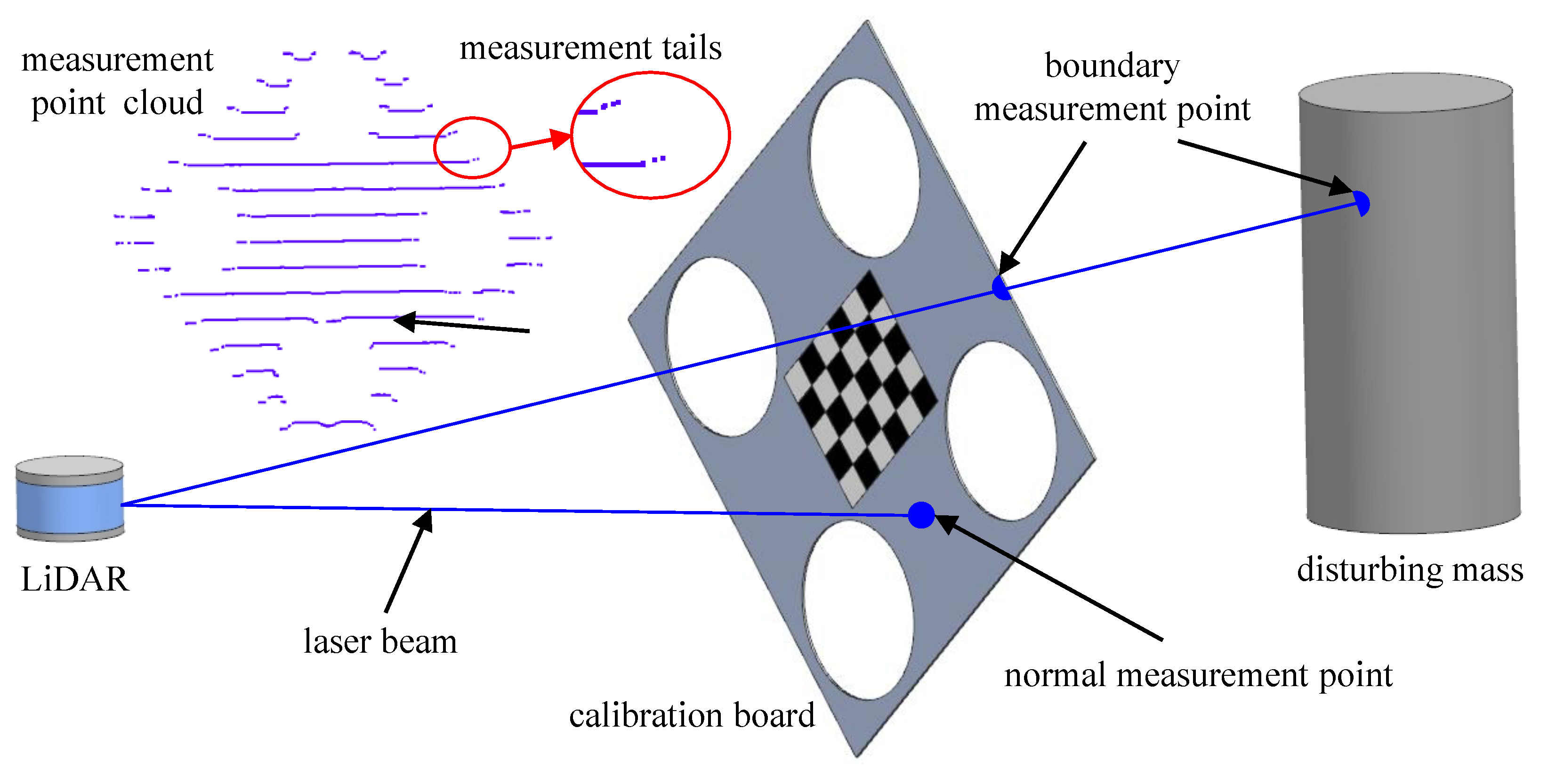
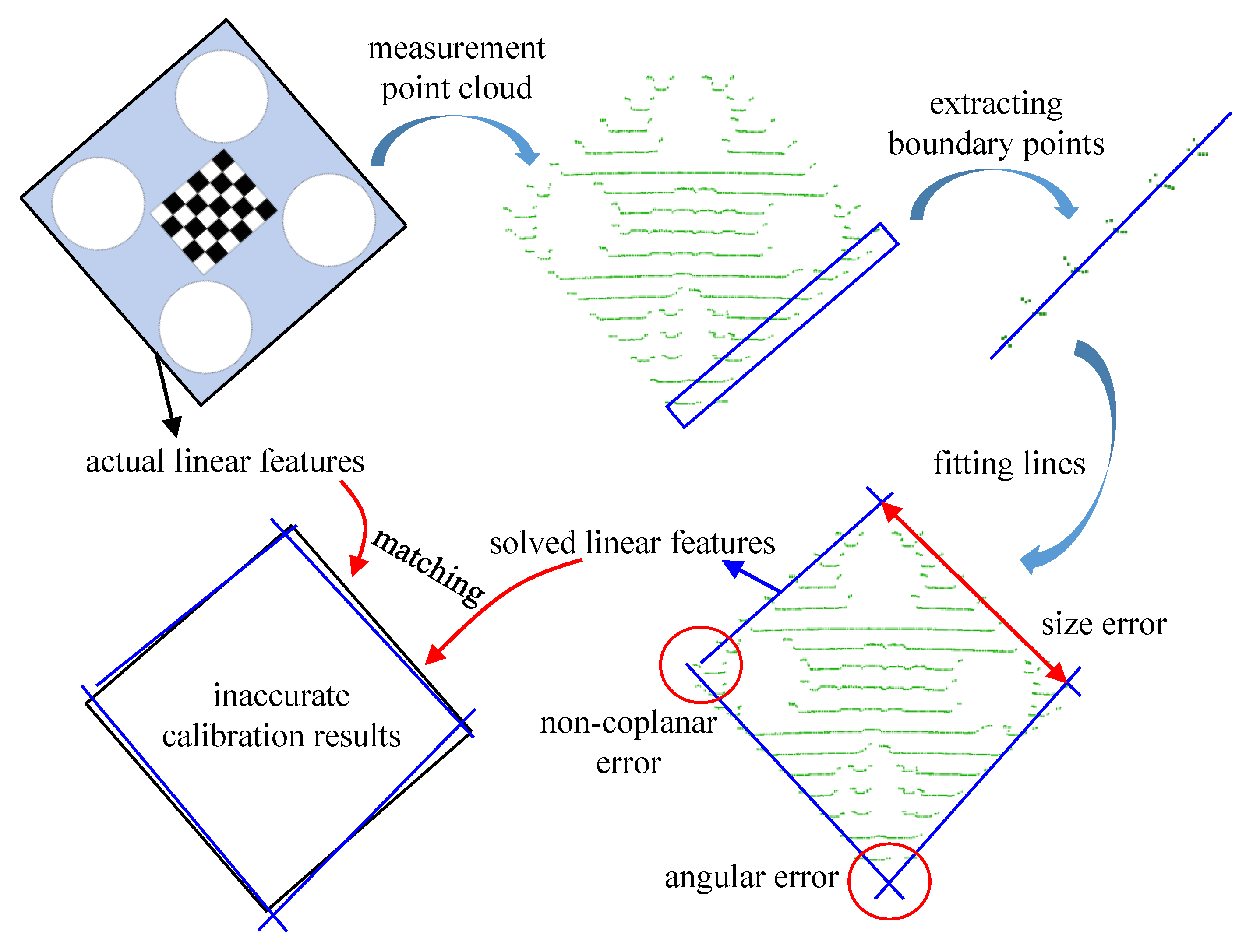
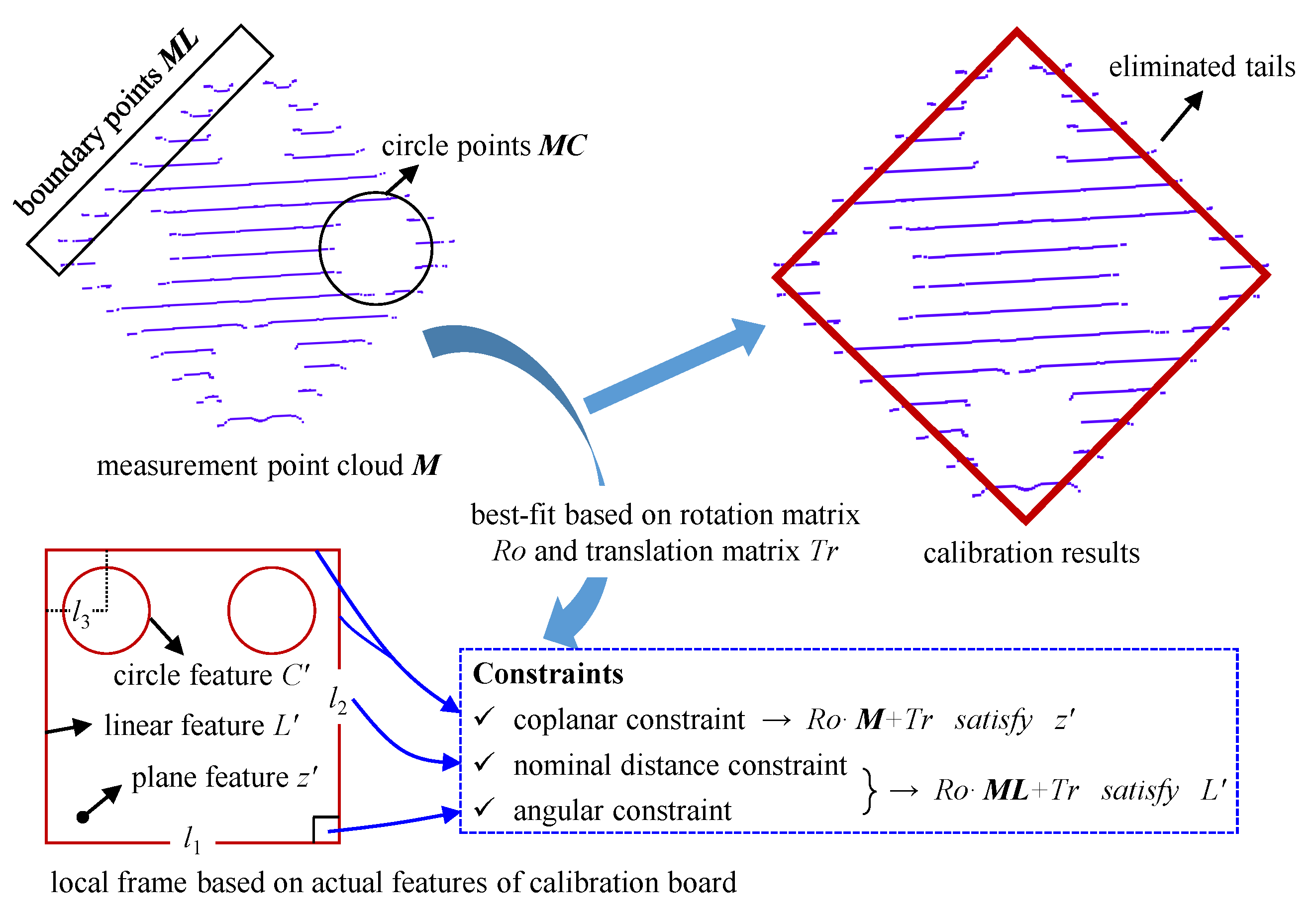
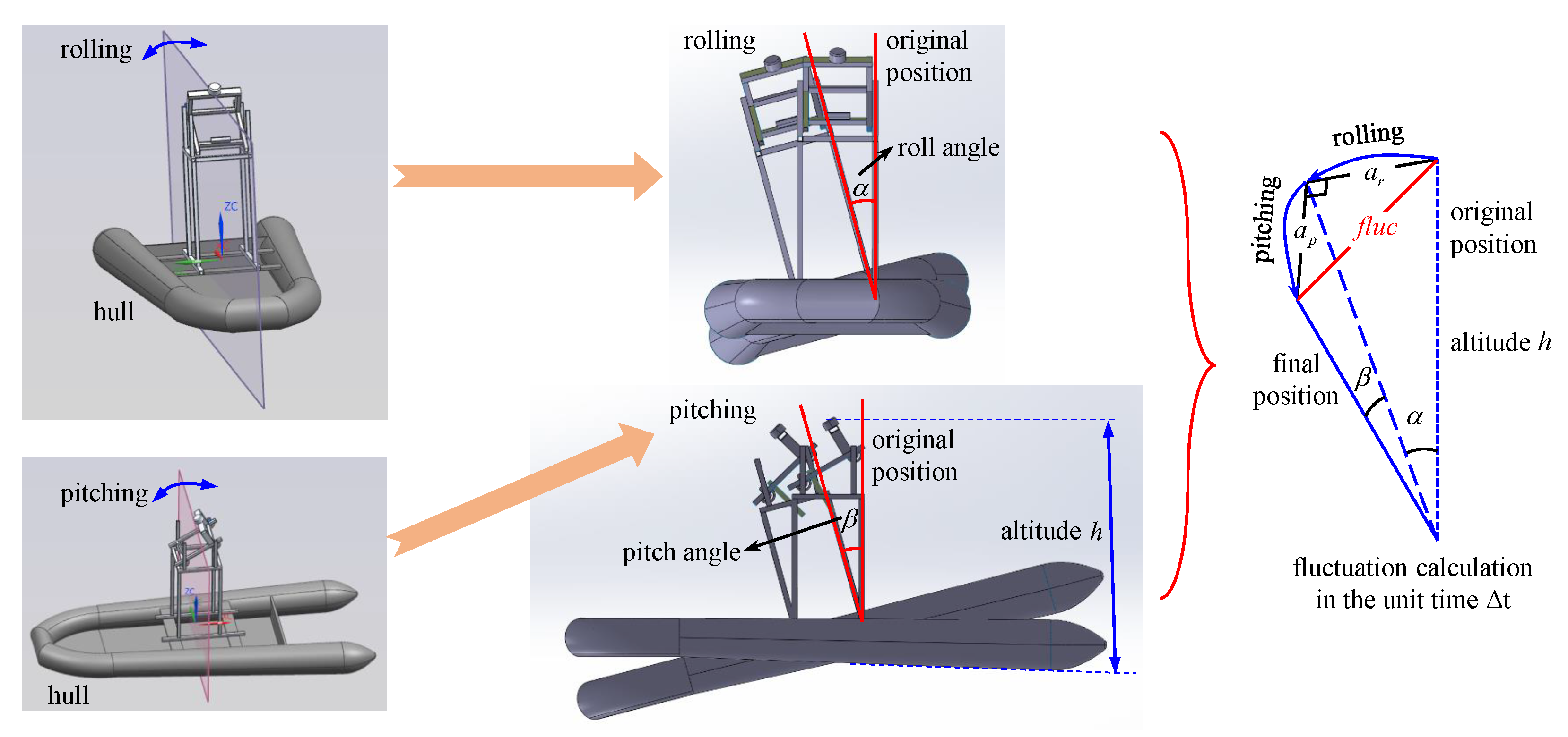
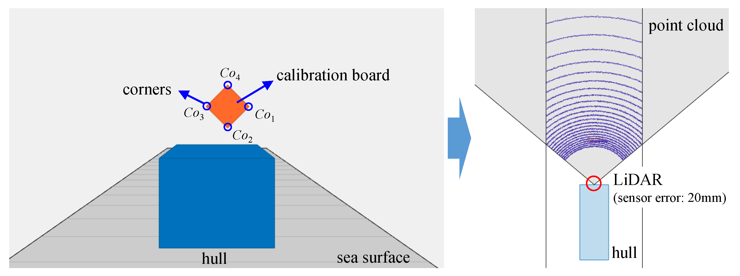
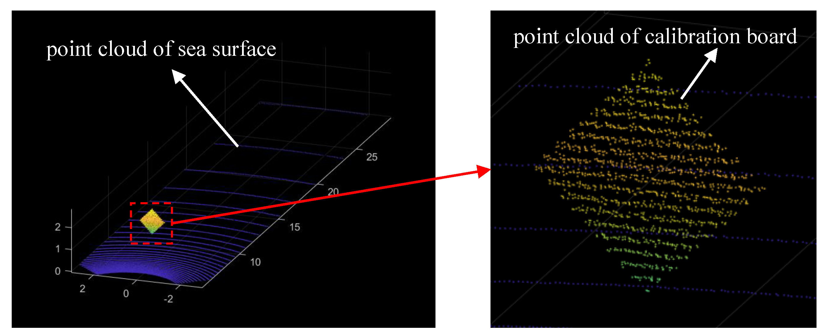
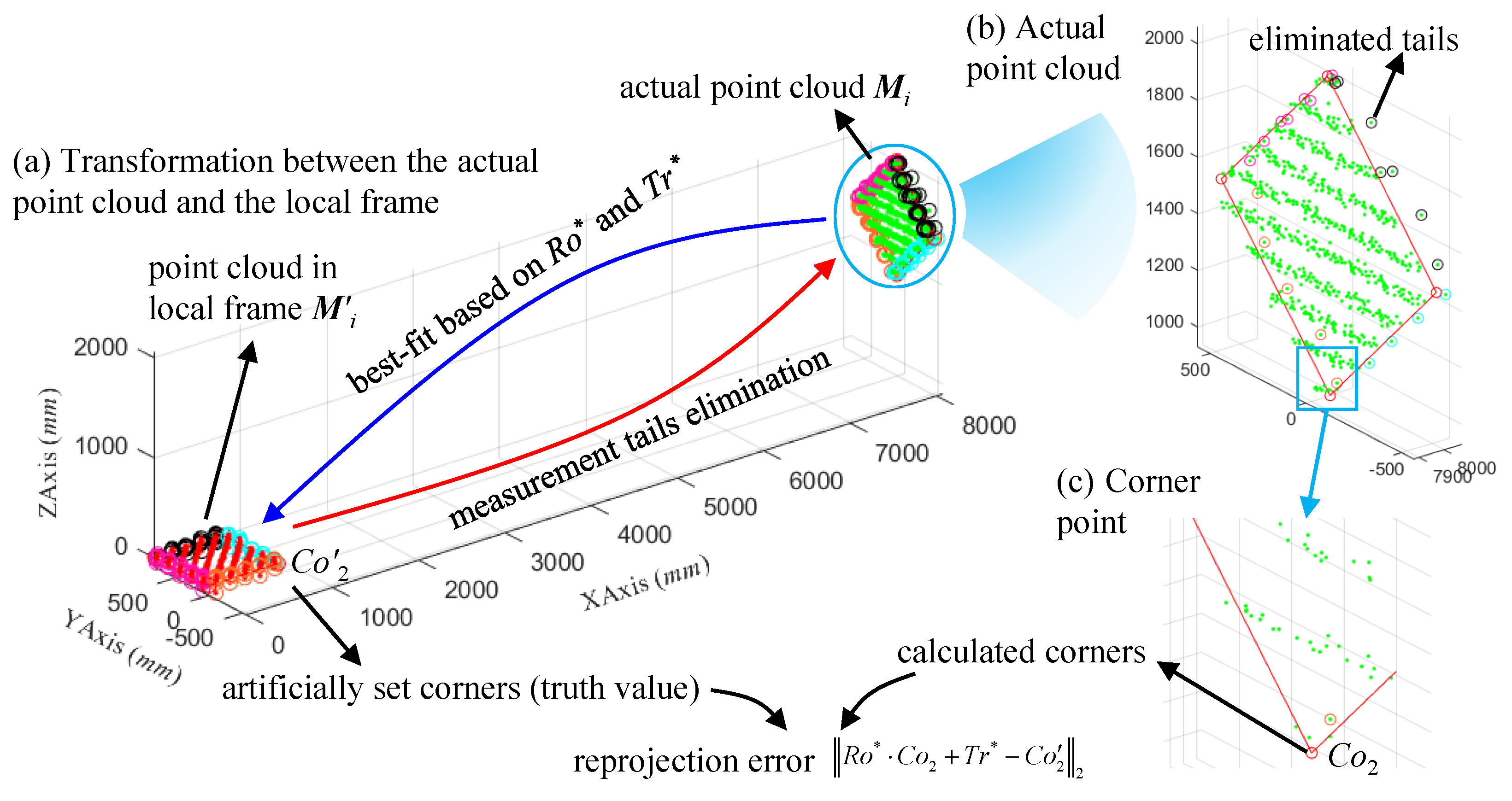
3.1. Accuracy Evaluation Model of LiDAR Measurements

Since the measurement points are actually circular in the LiDAR measurement process, measurement tails are inevitable, as shown in Figure 1, which directly affect the calibration accuracy of LiDAR systems and subsequently lead to a reduction in the spatial pose measurement accuracy.

Figure 1. Tails in LiDAR measurement process.

In traditional calibration procedures, as shown in Figure 2, the boundary point cloud is directly fitted to solve geometric features. However, the large number of measurement tails in the boundary point cloud severely interferes with the calibration accuracy, making non-coplanar, angular, and size errors in the solved linear features.

Figure 2. Traditional LiDAR calibration procedure.

Therefore, the coplanar, angular, and nominal distance constraints of the linear features on the calibration board are introduced, and the best-fit method is employed to suppress the interference of the measurement tails, which enables high-precision calibration of the LiDAR. Figure 3 details the proposed method.

Figure 3. The proposed LiDAR calibration procedure.

The coordinates of the point cloud collected by the LiDAR are defined as Equation (1).

$$\begin{array}{c}\hfill {\mathit{M}}_i={(x_i,y_i,z_i)}^T\\ \hfill {\mathit{ML}}_i,{\mathit{MC}}_i\subset \left\{{\mathit{M}}_i\right\}\end{array}$$

(1)

where ${\mathit{M}}_i$ is the ith point in point cloud $\left\{{\mathit{M}}_i\right\}$ with coordinate value ${(x_i,y_i,z_i)}^T$ and ${\mathit{ML}}_i$ and ${\mathit{MC}}_i$ represent the boundary point and circle point in $\left\{{\mathit{M}}_i\right\}$, respectively.

Meanwhile, a local frame is established, and a simple planar equation is employed to describe the calibration board, as shown in Equation (2), where the linear features and the circle features can be described as Equation (3).

$$z^{\prime }=0$$

(2)

$$\left\{\begin{array}{cc}\hfill L_1^{\prime }:& z^{\prime }=0,y^{\prime }=0\hfill \\ \hfill L_2^{\prime }:& z^{\prime }=0,x^{\prime }=l_1\hfill \\ \hfill L_3^{\prime }:& z^{\prime }=0,y^{\prime }=l_2\hfill \\ \hfill L_4^{\prime }:& z^{\prime }=0,x^{\prime }=0\hfill \end{array}\right.\left\{\begin{array}{cc}\hfill C_1^{\prime }& =(l_3,l_3,0)\hfill \\ \hfill C_2^{\prime }& =(l_1-l_3,l_3,0)\hfill \\ \hfill C_3^{\prime }& =(l_1-l_3,l_2-l_3,0)\hfill \\ \hfill C_4^{\prime }& =(l_3,l_2-l_3,0)\hfill \end{array}\right.$$

(3)

where $L_1^{\prime },L_2^{\prime },L_3^{\prime },L_4^{\prime }$ denote the line equations for boundaries of the calibration board, $C_1^{\prime },C_2^{\prime },C_3^{\prime },C_4^{\prime }$ denote the circle centers of the calibration board, $l_1,l_2,l_3$ are the dimension parameters of the calibration board as shown in Figure 3, and $(x^{\prime },y^{\prime },z^{\prime })$ is the coordinate value in the local frame.

To achieve the best fitting of the measured point cloud to the calibration board, the rotation and translation matrices are introduced as in Equation (4).

$$\left\{\begin{array}{cc}\hfill Ro& =\left[\begin{array}{ccc}cos{\theta }_z& -sin{\theta }_z& 0\\ sin{\theta }_z& cos{\theta }_z& 0\\ 0& 0& 1\end{array}\right]\left[\begin{array}{ccc}cos{\theta }_y& 0& sin{\theta }_y\\ 0& 1& 0\\ -sin{\theta }_y& 0& cos{\theta }_y\end{array}\right]\left[\begin{array}{ccc}1& 0& 0\\ 0& cos{\theta }_x& -sin{\theta }_x\\ 0& sin{\theta }_x& cos{\theta }_x\end{array}\right]\hfill \\ \hfill Tr& ={\left[\begin{array}{ccc}{t}_x& t_y& t_z\end{array}\right]}^T\hfill \end{array}\right.$$

(4)

where $Ro$ and $Tr$ are the unknown rotation and translation matrices to be solved, ${\theta }_x,{\theta }_y,{\theta }_z$ are the rotation angle around the $x,y,z$ axis, and $t_x,t_y,t_z$ are the translation along the $x,y,z$ axis. Therefore, as the parameters of $Ro$ and $Tr$, $({\theta }_x,{\theta }_y,{\theta }_z,t_x,t_y,t_z)$ can be considered as the six unknowns to be solved.

Thus, in the local frame, point ${\mathit{M}}_i$ can be expressed as Equation (5).

$${\mathit{M}}_i^{\prime }=Ro·{\mathit{M}}_i+Tr$$

(5)

where ${\mathit{M}}_i^{\prime }$ is the corresponding point of ${\mathit{M}}_i$ in the local frame.

It is obvious that ${\mathit{M}}_i^{\prime }$ satisfy Equation (2), and the boundary points of ${\mathit{M}}_i^{\prime }$ satisfy Equation (3). Then, the constraints can be established as Equation (6).

$$\left\{\begin{array}{cc}\hfill Ro·{\mathit{M}}_i+Tr& satisfy{z}^{\prime }=0\hfill \\ \hfill Ro·{\mathit{ML}}_i+Tr& satisfy{L}_{line}^{\prime },line=(1,2,3,4)\hfill \end{array}\right.$$

(6)

Then, the LiDAR calibration problem becomes an optimization problem with ${\theta }_x$, ${\theta }_y$, ${\theta }_z$, $t_x$, $t_y$, $t_z$ in Equation (4) as the objective and Equation (6) as the constraints. This problem can be solved by an optimization algorithm such as Levenberg–Marquardt (LM) [33], and the solution of $({\theta }_x,{\theta }_y,{\theta }_z,t_x,t_y,t_z)$ can be expressed as Equation (7).

$$({\theta }_x,{\theta }_y,{\theta }_z,t_x,t_y,t_z)\to ({\theta }_x^{*},{\theta }_y^{*},{\theta }_z^{*},t_x^{*},t_y^{*},t_z^{*})$$

(7)

where $({\theta }_x^{*},{\theta }_y^{*},{\theta }_z^{*},t_x^{*},t_y^{*},t_z^{*})$ is the solution of $({\theta }_x,{\theta }_y,{\theta }_z,t_x,t_y,t_z)$.

Finally, the accuracy of the LiDAR system is evaluated by the reprojection errors at specific points, such as the corners and circle centers of the calibration board. Given the fact that the circle centers are easier to extract in actual experiments, the LiDAR accuracy validation model based on the circle centers is more recommended. The actual coordinates of the circle centers $C_{circle},circle=(1,2,3,4)$ can be extracted from $\left\{{\mathit{MC}}_i\right\}$, and the accuracy evaluation model of the LiDAR system can be defined as Equation (8).

$$eval=\frac{1}{4}\sum _{circle=1}^4\left|\right|R{o}^{*}·C_{circle}+T{r}^{*}-C_{circle}^{\prime }{\left|\right|}_2$$

(8)

where $eval$ is the accuracy evaluation index of LiDAR calibration, $R{o}^{*}$ and $T{r}^{*}$ are obtained from Equation (4) by substituting the optimization solution in Equation (4), and $\left|\right|·{\left|\right|}_2$ denotes the 2-norm of a vector.

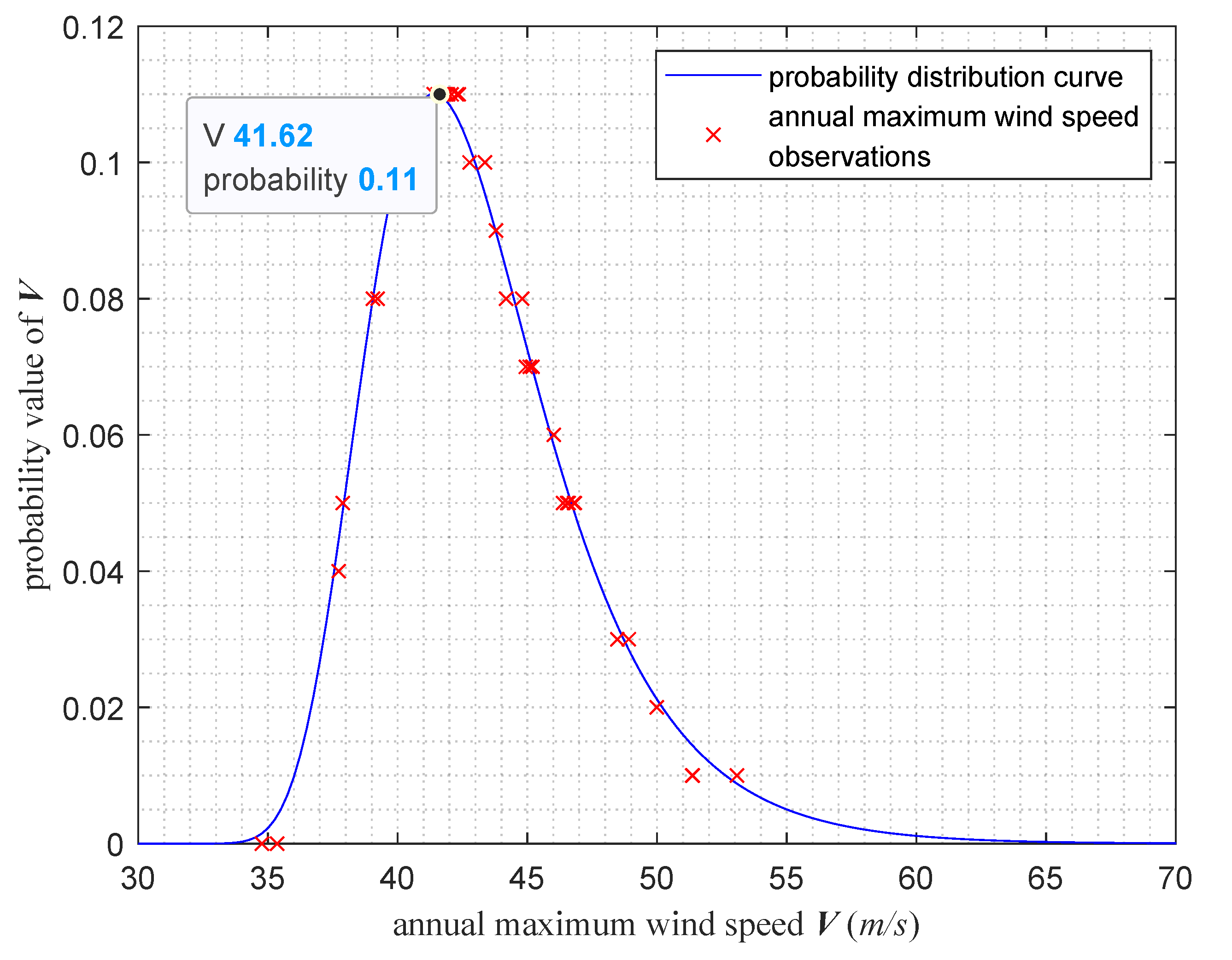
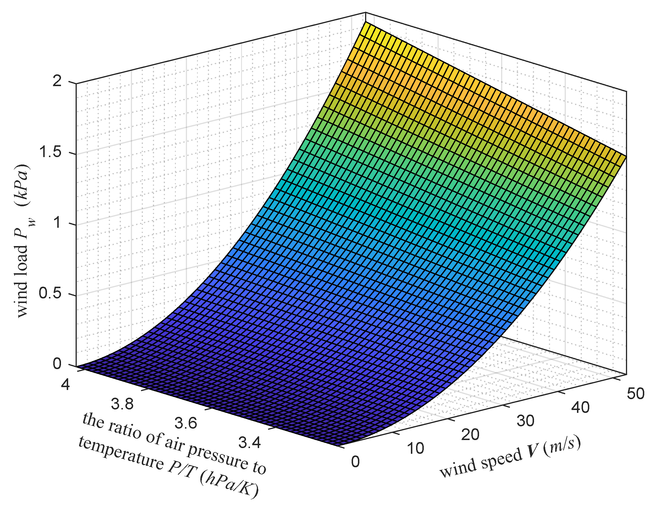
3.2. Establishment of Wind Load Probability Model

Due to the strong positive correlation between wind load and wind speed, only the annual maximum wind speed is analyzed statistically in this paper, and then an extreme wind load probability model is developed. The annual maximum wind speed is a typical stochastic variable and is considered by most statistical analyses to be subject to an I-type generalized extreme value distribution (Gumbel distribution) [34], as described in Equation (9).

$$H(\mathit{V};\mu ,\delta )=\frac{1}{\delta }{e}^{-\frac{\mathbf{V}-\mu }{\delta }}{e}^{-e^{-\frac{\mathit{V}-\mu }{\delta }}}$$

(9)

where $\mathit{V}=(V_1,V_2,\cdots )$ represents the annual maximum wind speed, e is the natural constant, and

$$\left\{\begin{array}{cc}\hfill \delta & =\frac{\sqrt{6}}{\pi }{V}_{mse}\hfill \\ \hfill \mu & =V_{mean}-0.5772\delta \hfill \end{array}\right.$$

(10)

where $V_{mse}$ and $V_{mean}$ are the mean squared error and mean value of the annual maximum wind speed $\mathit{V}$, respectively.

It is important to note that the wind speed measurements from the weather station are taken at a specific altitude, while the actual wind speed varies with altitude, which directly affects the wind load on the hull. Before calculating the wind load, it is therefore necessary to convert the annual maximum wind speed at the specific altitude into wind speeds at different altitudes, as indicated in Equation (11).

$${\mathit{V}}_{\mathit{h}}=\frac{lgh-lg{h}_0}{1g{h}_s-lg{h}_0}\mathit{V}$$

(11)

where h is the altitude, ${\mathit{V}}_{\mathit{h}}$ represents the wind speed at h, $h_s$ is the specific altitude at which the weather station collects the wind speed, and $h_0$ is the altitude at zero wind speed.

Then, the wind load can be expressed as follows in Equation (12).

$${\mathit{P}}_w=\frac{\rho {\mathit{V}}_{\mathit{h}}^2}{2}$$

(12)

where ${\mathit{P}}_w$ denotes the wind load and $\rho$ is the density of the atmosphere, which is related to the pressure and temperature as shown in Equation (13).

$$\rho =\frac{P}{P_0}\frac{T_0}{T}{\rho }_0$$

(13)

where P and T are the actual air pressure and temperature, respectively, and ${\rho }_0$ is the standard atmospheric density at standard air pressure $P_0$ and standard air temperature $T_0$.

From this, the wind load probability model with Equation (9) as the probability distribution and Equation (12) as the wind load can be obtained. It can be seen from Equations (12) and (13) that the wind speed, pressure, and temperature should be taken into account simultaneously to ensure the accuracy of the expression of the wind load probability model.

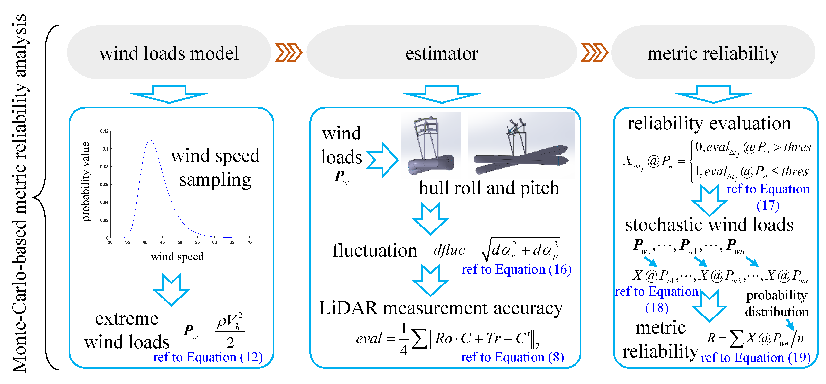
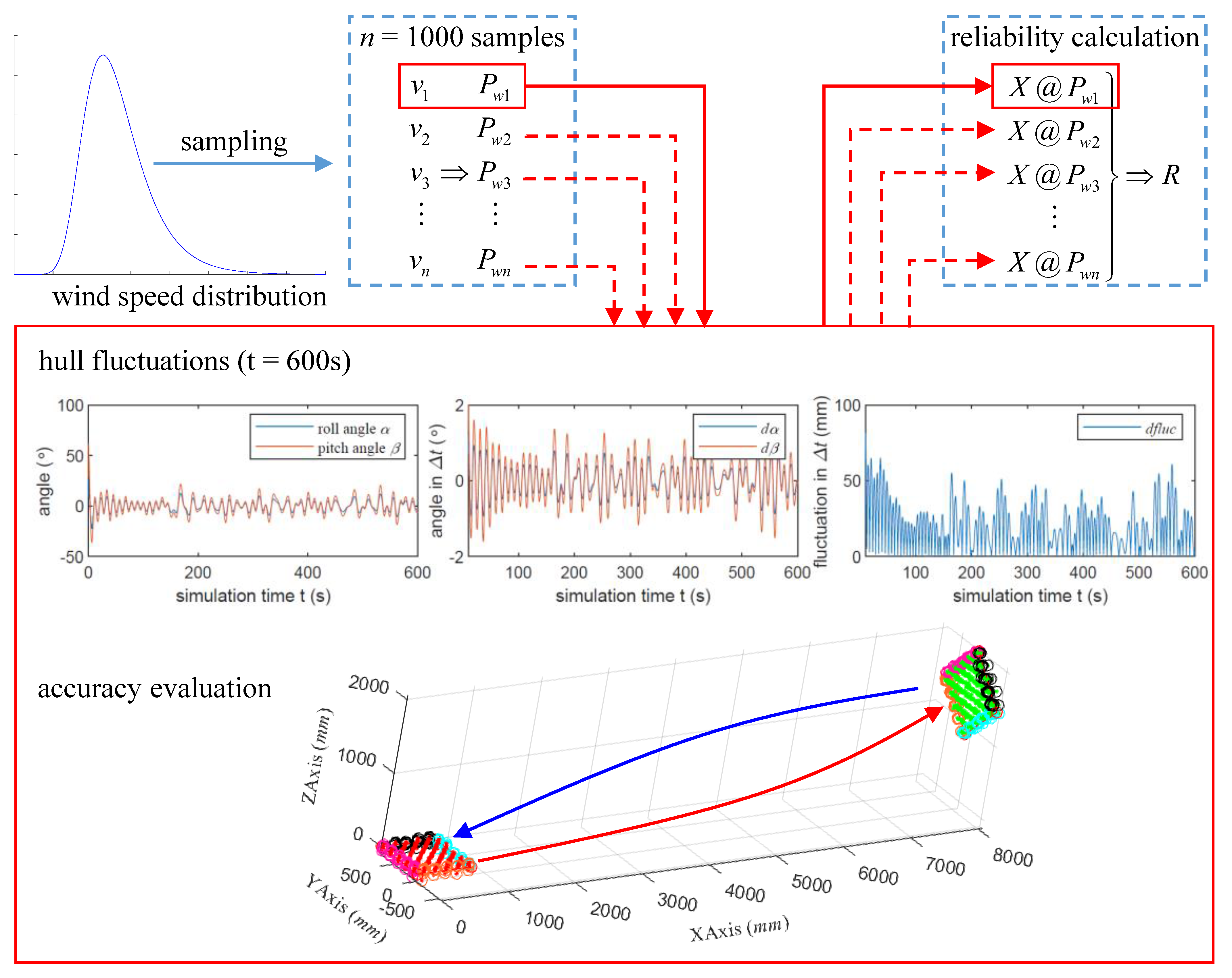
3.3. Monte-Carlo-Based Metric Reliability Analysis

The Monte-Carlo-based metric reliability analysis is performed in three stages. First, extreme wind loads are built by sampling from the probability distribution of the annual maximum wind speed. Then, the roll and pitch of the hull under the wind load are estimated, the maximum amplitude of the ship vibration per unit time is taken as the fluctuation of the LiDAR measurements, and the accuracy of the LiDAR measurements is evaluated by simulation analysis. Finally, the reliability evaluation function is established to calculate the reliability of the LiDAR system. The process of Monte-Carlo-based metric reliability analysis is shown in Figure 4.

Figure 4. The process of Monte-Carlo-based metric reliability analysis.

Establishing the extreme wind load can be performed using Equations (9) and (12), and then the simulation can be used to calculate the roll and pitch curves of the hull over time. For analytical ease, the unit time is defined as follows.

$$\mathsf{\Delta }t=\frac{1}{f}$$

(14)

where $\mathsf{\Delta }t$ is the unit time, which is equal to the time it takes LiDAR to measure one frame of data, and f is the LiDAR frame rate.

The roll and pitch of the hull during the unit time $\mathsf{\Delta }t$ are shown in Figure 5, where $\alpha$ and $\beta$ are the hull roll angle and pitch angle, respectively, $a_r$ and $a_p$ are the roll amplitude and pitch amplitude, h is the altitude, and $fluc$ represents the position fluctuation between the initial position and final position after the hull rolling and pitching.

Figure 5. Rolling and pitching of the hull during the unit time $\mathsf{\Delta }t$.

It is clear that the roll angle and pitch angle can be further expressed as $d\alpha$ and $d\beta$ in the unit time $\mathsf{\Delta }t$. Similarly, the amplitude per unit time can be expressed as $d{a}_r$ and $d{a}_p$, and the fluctuation per unit time can be expressed as $dfluc$. Thus, Equations (15) and (16) can be obtained from the spatial geometry shown in Figure 5.

$$\left\{\begin{array}{c}\hfill d{a}_r=2hsin\frac{d\alpha }{2}\\ \hfill d{a}_p=2hsin\frac{d\beta }{2}\end{array}\right.$$

(15)

$$dfluc=\sqrt{d{a}_r^2+d{a}_p^2}=2h\sqrt{{\left(sin\frac{d\alpha }{2}\right)}^2+{\left(sin\frac{d\beta }{2}\right)}^2}$$

(16)

The LiDAR measurement process under the fluctuation $dfluc$ is then simulated, and the metric accuracy is evaluated using Equation (8). Further, the reliability evaluation function in the unit time $\mathsf{\Delta }t$ under a special wind load is built as Equation (17).

$$X_{\mathsf{\Delta }{t}_j}@P_w=\left\{\begin{array}{c}0,eva{l}_{\mathsf{\Delta }{t}_j}@P_w>thres\hfill \\ 1,eva{l}_{\mathsf{\Delta }{t}_j}@P_w\le thres\hfill \end{array}\right.,j=1,2,\dots ,m$$

(17)

where $X_{\mathsf{\Delta }{t}_j}@P_w$ is the reliability evaluation indicator for LiDAR measurements in the unit time $\mathsf{\Delta }{t}_j$ under the special wind load $P_w$, $eva{l}_{\mathsf{\Delta }{t}_j}@P_w$ is the LiDAR measurement accuracy evaluation indicator, $thres$ is the measurement error threshold, and m is the number of units of time in the simulation experiment under the special wind load $P_w$.

Thus, the reliability evaluation indicator $X@P_w$ for LiDAR measurements under the special wind load $P_w$ can be expressed as Equation (18):

$$X@P_w=\sum _{j=1}^m{X}_{\mathsf{\Delta }{t}_j}@P_w/m$$

(18)

Since the sample distribution $H(\mathit{V};\mu ,\delta )$ has been taken into account in the sampling procedure in the Monte-Carlo method, the overall reliability R can finally be defined as the average of the reliability of each sample, as shown in Equation (19).

$$R=\sum _{k=1}^{n}X@P_w/n$$

(19)

where n is the sample size sampled from the extreme wind loads ${\mathit{P}}_w$.

4. Experiments

The implementation process is divided into three phases. First, according to Section 3.1, the static accuracy of the LiDAR system is evaluated. Then, the sea surface wind field data are investigated, the wind speed distribution is analyzed using Section 3.2, and the effect of wind speed, altitude, pressure, and temperature on the wind load is determined. Finally, the metric reliability of the LiDAR system is analyzed based on the Monte-Carlo method as described in Section 3.3.

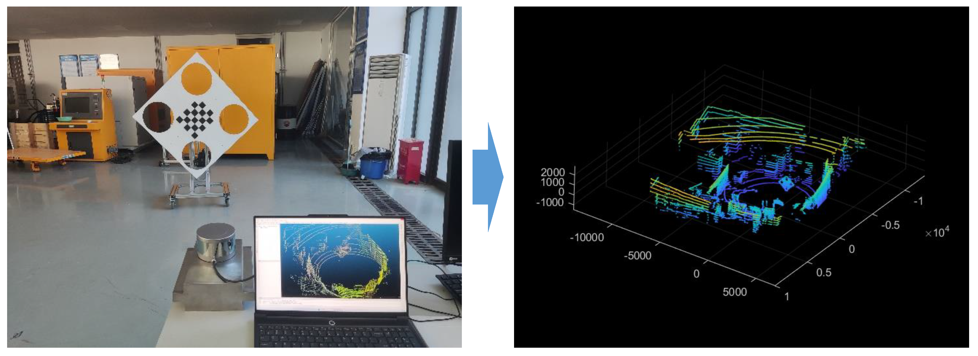
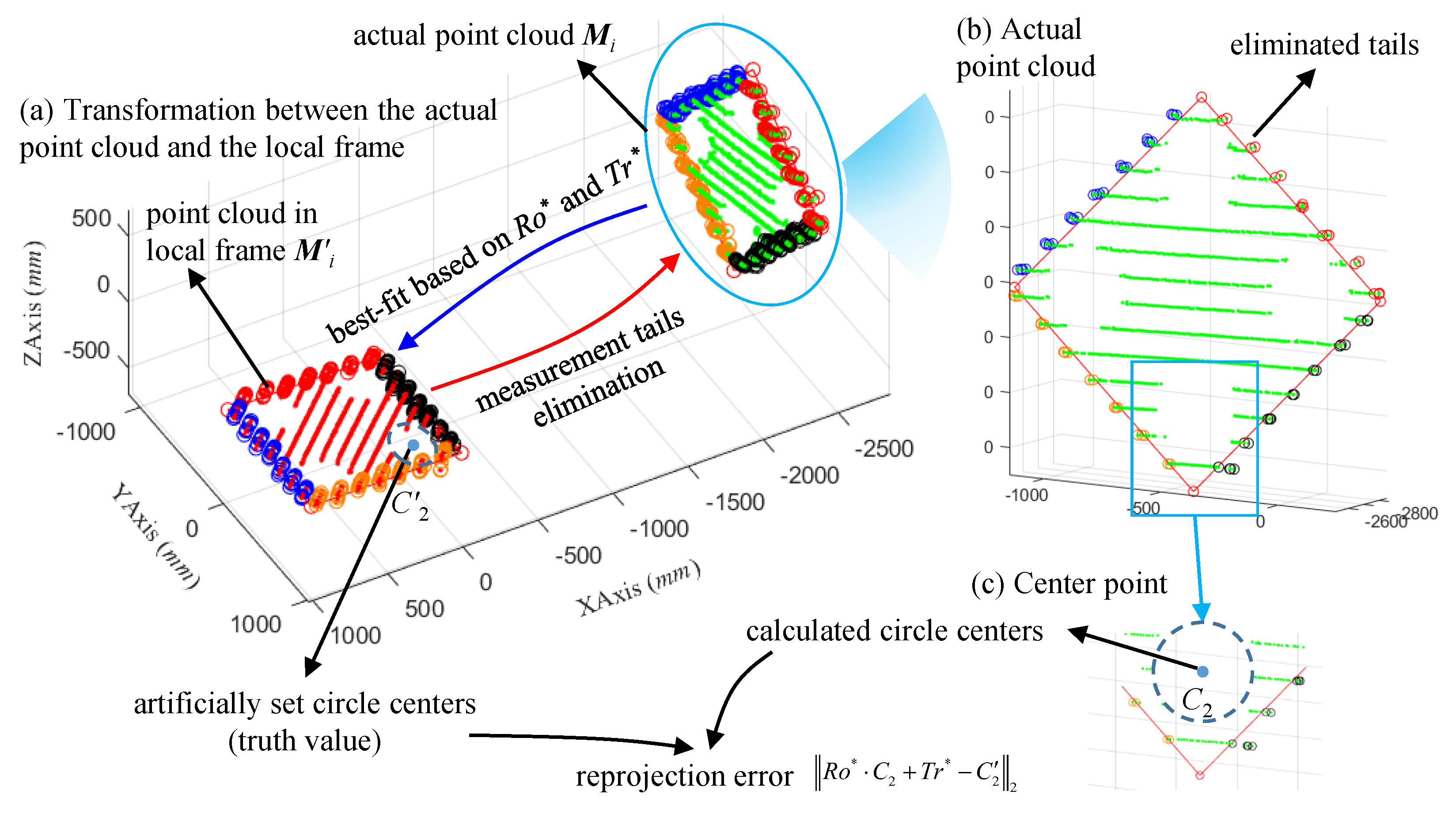
4.1. Accuracy Evaluation of LiDAR Measurements

Simulation and practical experiments are conducted to demonstrate the effectiveness of the proposed LiDAR point cloud tail elimination method, and the static measurement accuracy of the LiDAR system is evaluated in this section.

The simulation layout is shown in Figure 6, and the measurement point cloud is shown in Figure 7.

Figure 6. Simulation experiment layout.

Figure 7. The measurement point cloud in the simulation experiment.

Then, based on the simulated data, the accuracy of the LiDAR system is evaluated using the proposed method described in Section 3.1. Since the calibration board is artificially set and the corner coordinates are known in the simulation experiment, as shown in Figure 6, the more convenient corner errors are employed to evaluate the LiDAR accuracy. The accuracy evaluation process of LiDAR measurements is shown in Figure 8 and Table 1.

Figure 8. Accuracy evaluation process of LiDAR measurements in the simulation experiment.

Table 1. Accuracy evaluation of the LiDAR measurements in the simulation experiment.

Points		Coordinates in Local Frame (mm)	Distance Error (mm)
$C{o}_1$	truth value without tail elimination proposed method	$(0.000,0.000,0.000)$ $(8.507,4.141,-23.428)$ $(-4.604,1.759,-25.300)$	− $25.265$ $\mathbf{25}.\mathbf{775}$
$C{o}_2$	truth value without tail elimination proposed method	$(800.000,0.000,0.000)$ $(800.297,4.653,-23.854)$ $(795.275,4.724,-18.000)$	− $24.305$ $\mathbf{19}.\mathbf{200}$
$C{o}_3$	truth value without tail elimination proposed method	$(800.000,800.000,0.000)$ $(794.599,795.317,-36.694)$ $(793.154,804.038,-21.700)$	− $37.384$ $\mathbf{23}.\mathbf{110}$
$C{o}_4$	truth value without tail elimination proposed method	$(0.000,800.000,0.000)$ $(-0.145,801.305,-36.871)$ $(-3.970,803.965,1.000)$	− $36.894$ $\mathbf{5}.\mathbf{699}$
average	without tail elimination proposed method	−	$30.962$ $\mathbf{18}.\mathbf{446}$

Figure 8a shows the conversion results from the actual point cloud ${\mathit{M}}_i$ to the point cloud ${\mathit{M}}_i^{\prime }$ in the local frame based on the artificially set calibration board parameters. After identifying the measurement tails in the local frame, it is remapped to the actual point cloud to implement tails elimination, and the tails elimination result is shown in Figure 8b. Then, the linear characteristics of the boundaries of the actual point cloud are calculated, as well as their corners. Finally, the accuracy of LiDAR measurements is evaluated by the corner errors between the calculated value and the truth value, as shown in Table 1.

It can be seen from Table 1, after tail elimination based on the proposed method, the LiDAR measurement accuracy is significantly improved, and the average measurement error can be reduced from 30.962 mm to 18.446 mm, with a decrease of 40.42%.

Meanwhile, practical experiments are also conducted based on a LiDAR with the sensor error of 20 mm, as shown in Figure 9.

Figure 9. Practical experiment layout and the measurement point cloud.

Similarly, the measurement tails of the point cloud are eliminated by the proposed method and the reprojection error of the circle centers on the calibration board is employed as the evaluation metric for the accuracy of the LiDAR measurements. The results are shown in Figure 10 and Table 2.

Figure 10. Accuracy evaluation process of the LiDAR measurements in the practical experiment.

Table 2. Accuracy evaluation of the LiDAR measurements in the practical experiment.

Points		Coordinates in Local Frame (mm)	Distance Error (mm)
$C_1$	truth value without tail elimination proposed method	$(800.000,200.000,0.000)$ $(802.918,203.810,2.598)$ $(803.965,799.186,5.960)$	− $5.457$ $\mathbf{7}.\mathbf{205}$
$C_2$	truth value without tail elimination proposed method	$(200.000,200.000,0.000)$ $(191.261,200.463,5.402)$ $(798.258,196.155,4.929)$	− $10.284$ $\mathbf{6}.\mathbf{489}$
$C_3$	truth value without tail elimination proposed method	$(200.000,800.000,0.000)$ $(199.210,808.029,-10.491)$ $(200.553,198.327,6.746)$	− $13.234$ $\mathbf{6}.\mathbf{972}$
$C_4$	truth value without tail elimination proposed method	$(800.000,800.000,0.000)$ $(802.646,811.868,-6.506)$ $(200.675,797.495,8.117)$	− $13.790$ $\mathbf{8}.\mathbf{521}$
average	without tail elimination proposed method	−	$10.691$ $\mathbf{7}.\mathbf{299}$

Table 2 shows that the proposed method also performs well in the actual experiments, reducing the LiDAR measurement error by 31.73% from 10.691 mm to 7.299 mm and providing a good static measurement basis for reliable measurement of LiDAR systems under extreme wind loads.

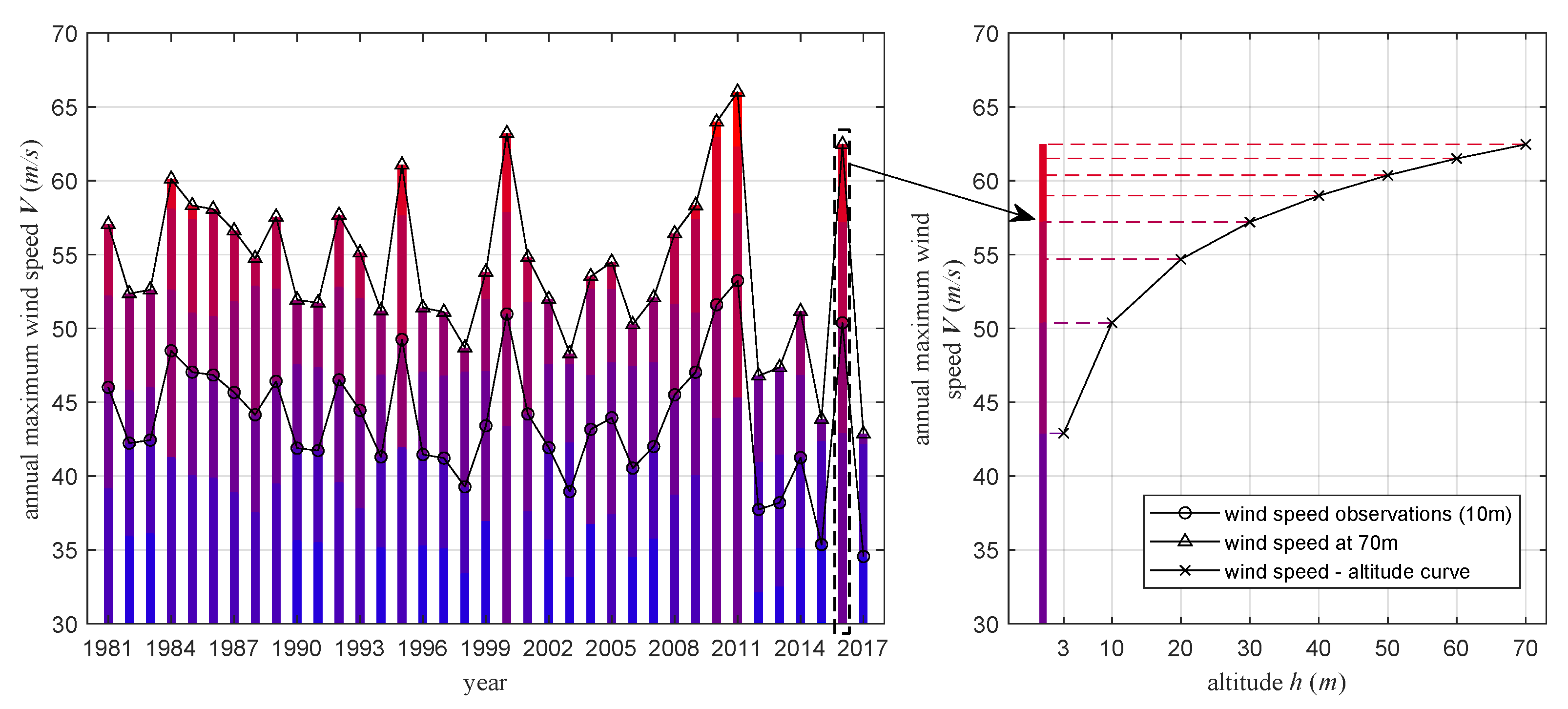
4.2. Sea Surface Wind Field Investigation and Wind Load Analysis

The probability distribution of the annual maximum wind speed was analyzed based on data on surface wind fields in the Pacific Northwest from 1981 to 2017. Some of the wind field data are given in Table 3.

Table 3. Some surface wind fields in the Pacific Northwest from 1980 to 2017.

Year	Annual Maximum Wind Speed V (m/s)	Air Pressure P ($\mathbf{hPa}$)	Air Temperature T (°C)
1981	45.8	998.0	−4.0
1982	41.7	990.2	3.0
1983	41.7	1006.0	10.2
…	…	…	…
2015	35.0	1012.2	1.0
2016	49.9	975.0	−2.0
2017	34.0	995.0	−2.0

Based on the wind field data, it is easy to calculate the mean squared error ($V_{mse}=4.29$ m/s) and the mean value ($V_{mean}=43.33$ m/s) of the annual maximum wind speed, as well as the variable values in Equation (10), as shown in Equation (20).

$$\left\{\begin{array}{cc}\hfill V_{mse}& =4.29\mathrm{m}/\mathrm{s}\hfill \\ \hfill V_{mean}& =43.33\mathrm{m}/\mathrm{s}\hfill \end{array}\right.⟹\left\{\begin{array}{cc}\hfill \delta & =3.34\mathrm{m}/\mathrm{s}\hfill \\ \hfill \mu & =41.40\mathrm{m}/\mathrm{s}\hfill \end{array}\right.$$

(20)

Thus, the resulting annual maximum wind speed distribution is shown in Figure 11, which provides the sampling probability for subsequent reliability analysis. As can be seen from Figure 11, the annual maximum wind speed is concentrated between 35 m/s and 60 m/s and the probability of occurrence of wind speed $41.62$ m/s is the largest, reaching about 11%.

Figure 11. Probability distribution curve of the annual maximum wind speed.

Then, in order to apply the corresponding wind load to different heights of the hull in the reliability analysis, the trend of the wind speed with height is investigated. The curve of wind speed versus altitude based on the annual maximum wind speed value (observed at 10 m) is shown in Figure 12. Finally, wind loads at different wind speeds, air pressures, and temperatures were calculated to provide load data for reliability analysis, as shown in Figure 13.

Figure 12. Curve of the wind speed as a function of altitude.

Figure 13. Curve of wind load with wind speed, air pressure, and temperature.

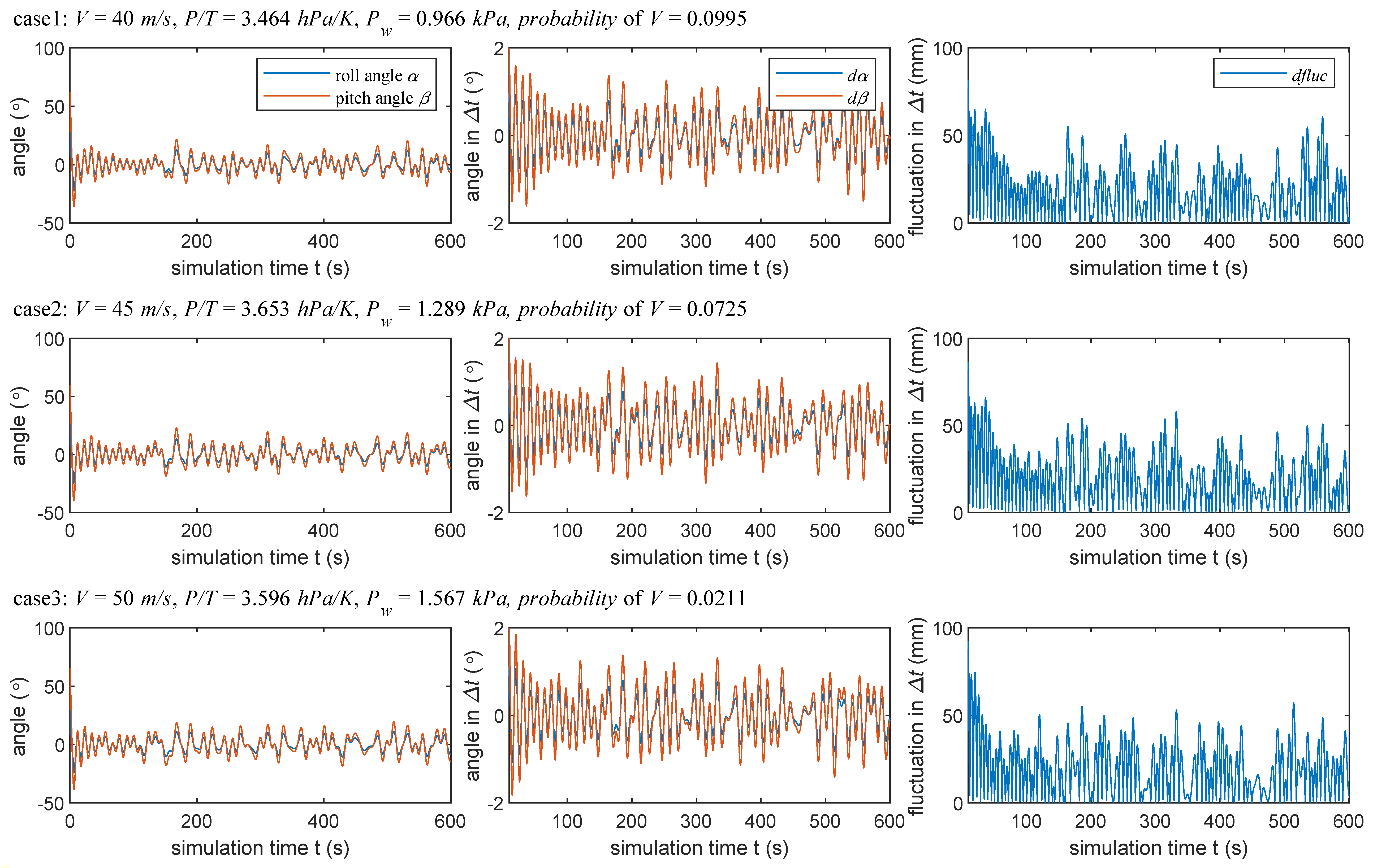
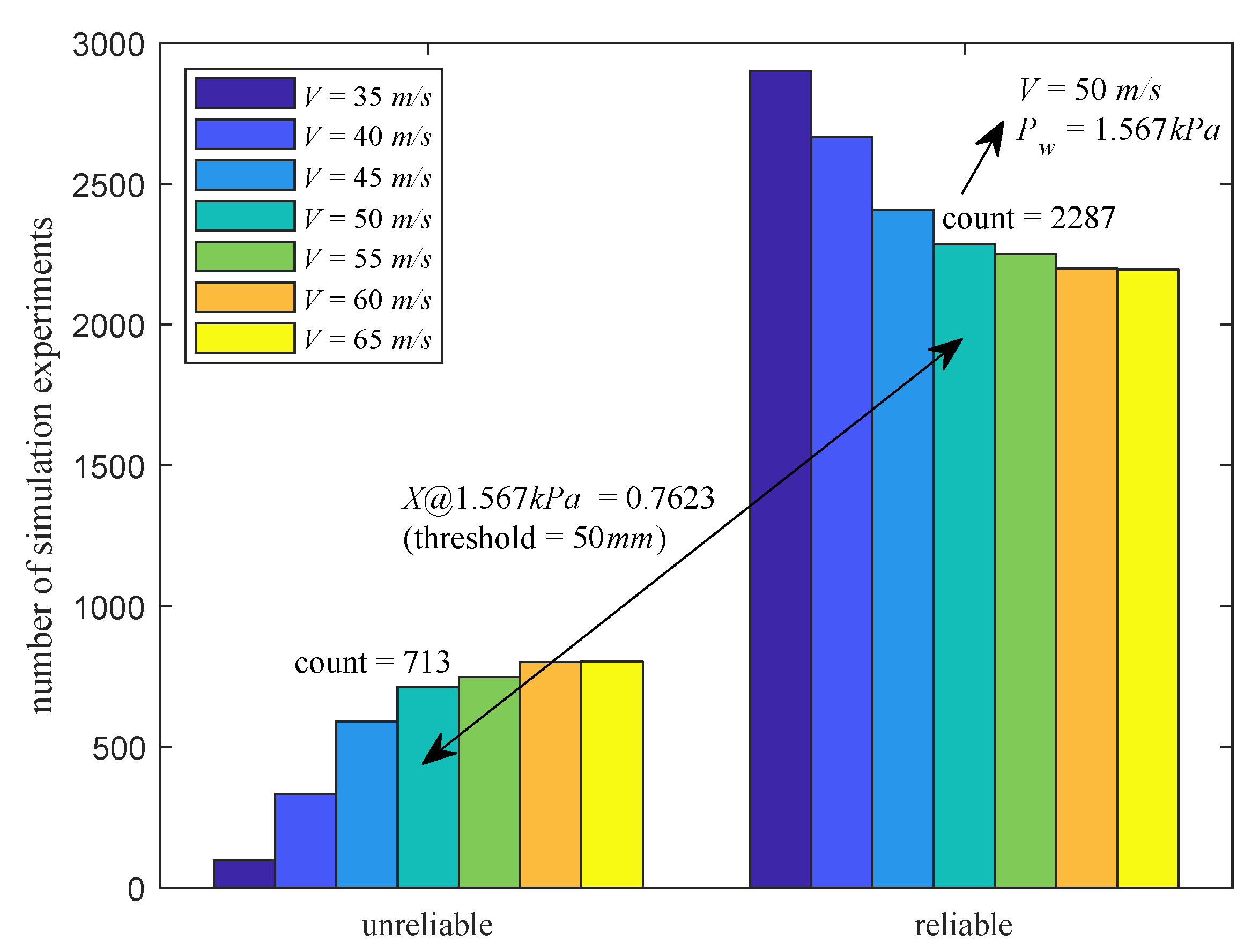
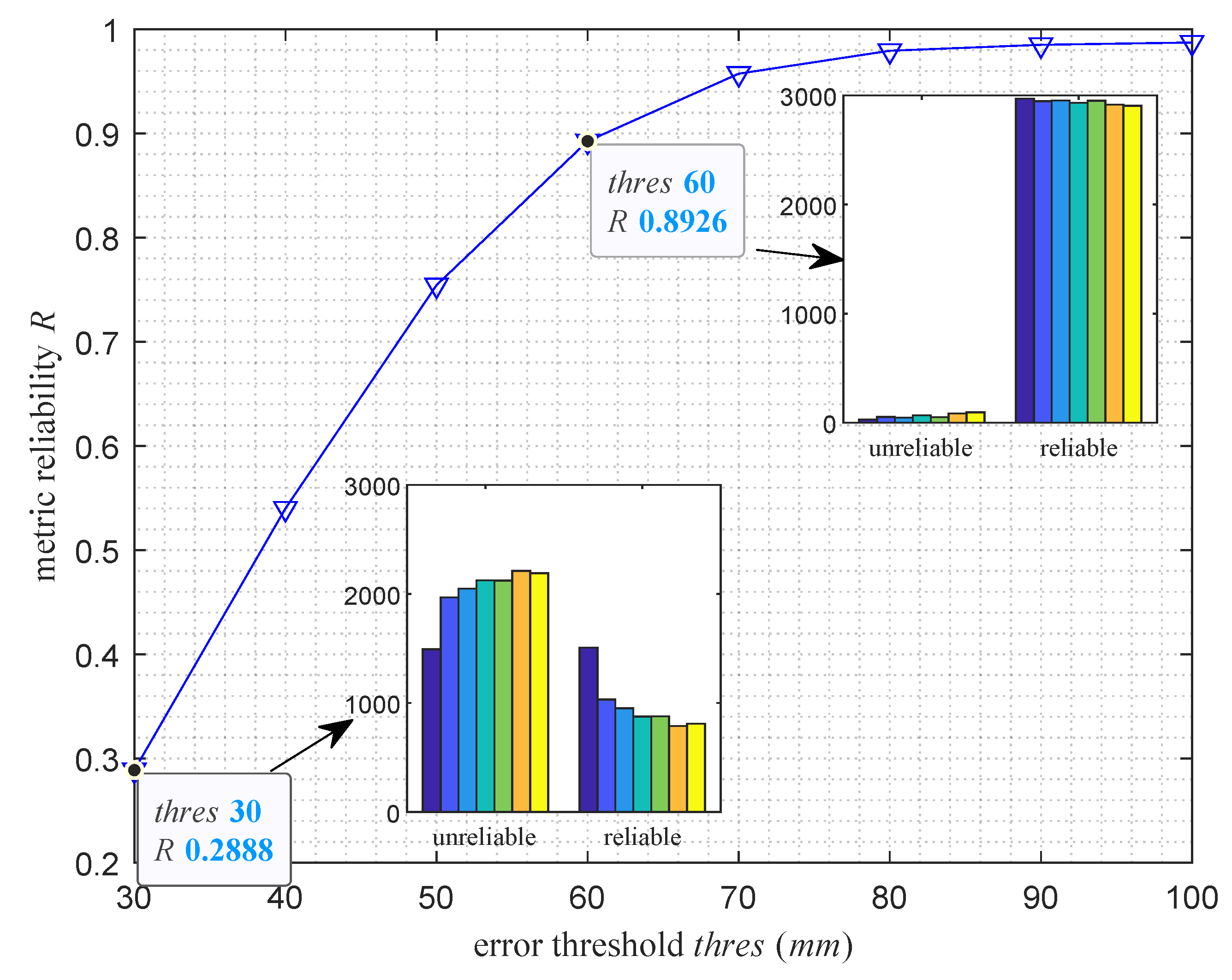
4.3. Metric Reliability Analysis of LiDAR Systems under Extreme Wind Loads

As described in Section 3.3 and Figure 4, the metric reliability analysis is performed in three steps: wind loads establishment, LiDAR measurement accuracy evaluation, and metric reliability calculation. The overall simulation procedure and configuration are shown in Figure 14.

Figure 14. The overall simulation procedure and configuration.

First, during the wind loads establishment process, $n={10}^4$ sets of the wind speeds are sampled from the probability distribution of the annual maximum wind speed shown in Figure 11, and then the wind loads are calculated according to Equation (12).

Then, each wind load is continuously applied to the hull for 10 min, and the roll and pitch characteristic curves of the hull are solved based on the MATLAB simulation platform. During the simulation, the LiDAR frame rate is set to $f=5$ Hz such that the unit time of the measurement is $\mathsf{\Delta }t=0.2$ s. Since the fluctuations of the hull in $\mathsf{\Delta }t$ directly affect the accuracy of LiDAR measurements, the roll and pitch angles of the hull in $\mathsf{\Delta }t$ were further calculated, as well as the fluctuations of the hull in $\mathsf{\Delta }t$, and some of the results are shown in Figure 15. In addition, the distribution curve of the hull fluctuations under each wind load is shown in Figure 16.

Figure 15. Hull roll-pitch angle and fluctuation in unit time under some typical wind load samples.

Figure 16. Hull fluctuation probability distribution in unit time.

Figure 16 shows that the fluctuations of the hull in unit time follow a normal distribution, with the amplitude of the fluctuations in unit time increasing as the wind load increases. The mean fluctuation in unit time under variable wind loads is $11.49$ mm to $24.74$ mm, and the maximum can reach $64.52$ mm to $158.96$ mm.

Finally, the metric reliability of LiDAR is analyzed. Represented by the wind loads at a range of typical wind speeds, Figure 17 shows the metric reliability calculation procedure and results when the allowed error threshold is $thres=50$ mm.

Figure 17. Simulation experiments with various wind loads (error threshold $thres=50$ mm).

It can be seen from Figure 17, in the case of a 50 m/s wind speed, that the wind load can reach $1.567$ kPa and 3000 time units are included in the 10 min simulation. Hull fluctuations in the unit time are applied to a simulated calibration board, and the accuracy of the LiDAR measurements is analyzed. In the 3000 simulation experiments, 713 of the LiDAR measurement errors exceed the set threshold, and the remaining 2287 meet the requirement. Thus, when the wind load reaches $1.567$ kPa, the reliability evaluation indicator $X@1.567$ kPa is calculated as $2287/3000=0.7623$.

The wind loads, occurrence probabilities, and reliability evaluation indicators for some typical extreme wind speeds are shown in Table 4, and the final metric reliability R is calculated according to Equation (4) for the threshold of 50 mm.

Table 4. Simulation results with various wind loads (error threshold $thres=50$ mm).

Annual Maximum Wind Speed $\mathit{V}$ (m/s)	Wind Load ${\mathit{P}}_{\mathit{w}}$ (kPa)	Probability of V	Indicator $\mathit{X}@{\mathit{P}}_{\mathit{w}}$	Reliability R
35	0.735	0.0023	0.9527	0.7540
40	0.966	0.0995	0.8690
45	1.289	0.0725	0.8080
50	1.567	0.0211	0.7623
55	1.966	0.0050	0.7647
60	2.340	0.0011	0.7300
65	2.958	0.0003	0.7540

Further, Figure 18 illustrates the metric reliabilities for different threshold values from 30 mm to 100 mm. It can be seen that when the threshold is low (high measurement accuracy is required), such as $thres=30$ mm, the reliability is only 0.2888, whereas when the threshold is relatively high, such as $thres=60$ mm, the reliability can reach 0.8926.

Figure 18. Curve of LiDAR metric reliability R versus error threshold $thres$.

5. Discussion

Metric reliability evaluation is of great guidance and preventive importance for the safe and stable operation of large equipment, such as marine LiDAR systems facing extreme wind loads. Thus, an evaluation procedure was proposed in this paper for the metric reliability of marine LiDAR systems under extreme wind loads, which consists of the following three steps. First, the static measurement accuracy of the LiDAR system was initially evaluated. However, due to the measurement properties of the LiDAR system, measurement tails will occur and severely interfere with the measurement results, as shown in Figure 1. Therefore, measurement tails should be eliminated to improve the static measurement accuracy of the marine LiDAR and thus provide a good data basis for dynamic measurements during the ship navigation. The proposed method can effectively remove the tails, as shown in Figure 10. The static measurement error was greatly reduced by simulation and laboratory experimental analysis, and the measurement accuracy was improved by 30–40%, as shown in Table 1 and Table 2. Second, offshore wind fields are investigated (Figure 11) and wind loads are calculated (Figure 13) to provide load data for reliability analysis of marine LiDAR measurements during navigation. Finally, the simulation and analysis of the hull fluctuation under extreme wind loads (Figure 15 and Figure 16) and its impact on the reliability of LiDAR measurements (Figure 17) were performed. In combination with the static accuracy evaluation method for LiDAR systems, the relationship curve between metric reliability and measurement accuracy was resolved, as shown in Figure 18. Experimental results show that the metric reliability of the LiDAR system is positively correlated with the allowed measurement error, with a reliability of above 0.89 for measurement errors less than 60 mm.

It can be believed that this study significantly contributes to the metric reliability analysis method for marine LiDAR systems. This study not only improves the LiDAR static measurement accuracy but also addresses the relationship between LiDAR metric reliability and measurement allowable errors. In addition, the proposed reliability evaluation process for marine LiDAR systems can be transferred to LiDAR-based driver assistance systems and robotic systems to provide guidance and preventative significance for the safe and stable operation of the devices.

6. Conclusions

Marine LiDAR systems play an important role in ensuring the safe navigation of ships, and it is important to evaluate the accuracy and reliability of marine LiDAR measurements. In this paper, a metric reliability analysis method was proposed for marine LiDAR systems under extreme wind loads. First, an evaluation model for the static measurement accuracy of LiDAR systems was developed, which eliminated the measurement tail problem caused by the LiDAR measurement properties and improved the static measurement accuracy by 30–40%. Second, wind fields in the Pacific Northwest were investigated, and the Gumbel distribution was used to describe the distribution of extreme wind speeds and to develop a wind load probability model. Finally, based on the wind load probability model, the hull fluctuations were simulated, and the impact of hull fluctuations on the reliability of LiDAR measurements was analysed. Based on the Monte-Carlo method and static accuracy evaluation of LiDAR systems, the correlation between the metric reliability and measurement accuracy of marine LiDAR system was analyzed under extreme wind loads. Results indicate that the metric reliability of the marine LiDAR system increases with the increase of the allowable value of measurement error, and the metric reliability reaches more than 0.89 when the measurement error is 60 mm, which provides guiding significance for the metric reliability of marine LiDAR systems in the process of ship navigation. In the course of this study, only the metric reliability of the marine LiDAR systems under extreme wind loads in the Pacific Northwest was analyzed, which is not sufficient for ship navigation. However, the proposed method is generally applicable, so the corresponding experiments in other offshore wind conditions will be performed in future work.

References

- Lee, P.; Theotokatos, G.; Boulougouris, E.; Bolbot, V. Risk-Informed Collision Avoidance System Design for Maritime Autonomous Surface Ships. Ocean Eng. 2023, 279, 113750. [Google Scholar] [CrossRef]
- Zhang, D.; Han, Z.; Zhang, K.; Zhang, J.; Zhang, M.; Zhang, F. Use of Hybrid Causal Logic Method for Preliminary Hazard Analysis of Maritime Autonomous Surface Ships. J. Mar. Sci. Eng. 2022, 10, 725. [Google Scholar] [CrossRef]
- Zhang, M.; Zhang, D.; Yao, H.; Zhang, K. A Probabilistic Model of Human Error Assessment for Autonomous Cargo Ships Focusing on Human-Autonomy Collaboration. Saf. Sci. 2020, 130, 104838. [Google Scholar] [CrossRef]
- Clunie, T.; DeFilippo, M.; Sacarny, M.; Robinette, P. Development of a Perception System for an Autonomous Surface Vehicle using Monocular Camera, LIDAR, and Marine RADAR. In Proceedings of the 2021 IEEE International Conference on Robotics and Automation (ICRA), Xi’an, China, 30 May–5 June 2021; pp. 14112–14119. [Google Scholar] [CrossRef]
- Lee, S.J.; Moon, Y.S.; Ko, N.Y.; Choi, H.T.; Lee, J.M. A Method for Object Detection Using Point Cloud Measurement in the Sea Environment. In Proceedings of the 2017 IEEE Underwater Technology (UT), Busan, Republic of Korea, 21–24 February 2017. [Google Scholar] [CrossRef]
- Stanislas, L.; Dunbabin, M. Multimodal Sensor Fusion for Robust Obstacle Detection and Classification in the Maritime RobotX Challenge. IEEE J. Ocean. Eng. 2019, 44, 343–351. [Google Scholar] [CrossRef]
- Stateczny, A.; Kazimierski, W.; Burdziakowski, P.; Motyl, W.; Wisniewska, M. Shore Construction Detection by Automotive Radar for the Needs of Autonomous Surface Vehicle Navigation. ISPRS Int. J. Geo-Inf. 2019, 8, 80. [Google Scholar] [CrossRef]
- Han, J.; Cho, Y.; Kim, J.; Kim, J.; Son, N.s.; Kim, S.Y. Autonomous Collision Detection and Avoidance for ARAGON USV: Development and Field Tests. J. Field Robot. 2020, 37, 987–1002. [Google Scholar] [CrossRef]
- Wang, H.; Yin, Y.; Jing, Q. Comparative Analysis of 3D LiDAR Scan-Matching Methods for State Estimation of Autonomous Surface Vessel. J. Mar. Sci. Eng. 2023, 11, 840. [Google Scholar] [CrossRef]
- Hu, B.; Liu, X.; Jing, Q.; Lyu, H.; Yin, Y. Estimation of Berthing State of Maritime Autonomous Surface Ships based on 3D LiDAR. Ocean Eng. 2022, 251, 111131. [Google Scholar] [CrossRef]
- Chen, Y.; Chen, Y. Reliability Evaluation of Sight Distance on Mountainous Expressway Using 3D Mobile Mapping. In Proceedings of the 2019 5th International Conference on Transportation Information and Safety (ICTIS), Liverpool, UK, 14–17 July 2019; pp. 1024–1030. [Google Scholar] [CrossRef]
- Wen, X.; Hu, J.; Chen, H.; Huang, S.; Hu, H.; Zhang, H. Research on an Adaptive Method for the Angle Calibration of Roadside LiDAR Point Clouds. Sensors 2023, 23, 7542. [Google Scholar] [CrossRef]
- Canavosio-Zuzelski, R.; Hogarty, J.; Rodarmel, C.; Lee, M.; Braun, A. Assessing Lidar Accuracy with Hexagonal Retro-Reflective Targets. Photogramm. Eng. Remote Sens. 2013, 79, 663–670. [Google Scholar] [CrossRef]
- Nguyen, T.T.; Cheng, C.H.; Liu, D.G.; Le, M.H. Improvement of Accuracy and Precision of the LiDAR System Working in High Background Light Conditions. Electronics 2022, 11, 45. [Google Scholar] [CrossRef]
- Zhang, Y.; Wu, T.; Zhang, X.; Sun, Y.; Wang, Y.; Li, S.; Li, X.; Zhong, K.; Yan, Z.; Xu, D.; et al. Rayleigh Lidar Signal Denoising Method Combined with WT, EEMD and LOWESS to Improve Retrieval Accuracy. Remote Sens. 2022, 14, 3270. [Google Scholar] [CrossRef]
- Cheng, X.; Mao, J.; Li, J.; Zhao, H.; Zhou, C.; Gong, X.; Rao, Z. An EEMD-SVD-LWT Algorithm for Denoising a Lidar Signal. Measurement 2021, 168, 108405. [Google Scholar] [CrossRef]
- Tuley, J.; Vandapel, N.; Hebert, A. Analysis and Removal of Artifacts in 3-D LADAR Data. In Proceedings of the 2005 IEEE International Conference on Robotics and Automation (ICRA), Barcelona, Spain, 18–22 April 2005; pp. 2203–2210. [Google Scholar] [CrossRef]
- Cifuentes, R.; Van der Zande, D.; Salas, C.; Farifteh, J.; Coppin, P. Correction of Erroneous LiDAR Measurements in Artificial Forest Canopy Experimental Setups. Forests 2014, 5, 1565–1583. [Google Scholar] [CrossRef]
- Perez-Canosa, J.M.; Orosa, J.A.; Lamas Galdo, M.I.; Cartelle Barros, J.J. A New Theoretical Dynamic Analysis of Ship Rolling Motion Considering Navigational Parameters, Loading Conditions and Sea State Conditions. J. Mar. Sci. Eng. 2022, 10, 1646. [Google Scholar] [CrossRef]
- Htun, S.S.; Umeda, N.; Sakai, M.; Matsuda, A.; Terada, D. Water-on-deck effects on roll motions of an offshore supply vessel in regular stern quartering waves. Ocean Eng. 2019, 188, 106225. [Google Scholar] [CrossRef]
- Chou, J.S.; Truong, D.N. Multiobjective Optimization Inspired by Behavior of Jellyfish for Solving Structural Design Problems. Chaos Solitons Fractals 2020, 135, 109738. [Google Scholar] [CrossRef]
- Hostettler, R.; Schon, T.B. Auxiliary-Particle-Filter-based Two-Filter Smoothing for Wiener State-Space Models. In Proceedings of the 2018 21st International Conference on Information Fusion (FUSION), Cambridge, UK, 10–13 July 2018; pp. 1904–1911. [Google Scholar] [CrossRef]
- Esedoglu, S.; Jacobs, M. Convolution Kernels and Stability of Threshold Dynamics Methods. SIAM J. Numer. Anal. 2017, 55, 2123–2150. [Google Scholar] [CrossRef]
- Mahboub, V.; Ebrahimzadeh, S.; Saadatseresht, M.; Faramarzi, M. On Robust Constrained Kalman Filter for Dynamic Errors-in-Variables model. Surv. Rev. 2020, 52, 253–260. [Google Scholar] [CrossRef]
- Wei, Y.; Chen, Z.; Zhao, C.; Tu, Y.; Chen, X.; Yang, R. An Ensemble Multi-Step Forecasting Model for Ship Roll Motion under Different External Conditions: A Case Study on the South China Sea. Measurement 2022, 201, 111679. [Google Scholar] [CrossRef]
- Li, Y.; Wei, Z.; Kapitaniak, T.; Zhang, W. Stochastic Bifurcation and Chaos Analysis for a Class of Ships Rolling Motion under Non-Smooth Perturbation and Random Excitation. Ocean Eng. 2022, 266, 112859. [Google Scholar] [CrossRef]
- Wang, Y.; Yao, W.; Zhang, B.; Fu, J.; Yang, J.; Sun, G. DRR-LIO: A Dynamic-Region-Removal-Based LiDAR Inertial Odometry in Dynamic Environments. IEEE Sens. J. 2023, 23, 13175–13185. [Google Scholar] [CrossRef]
- Li, J.; Bi, Y.; Li, K.; Wu, L.; Cao, J.; Hao, Q. Improving the Accuracy of TOF LiDAR Based on Balanced Detection Method. Sensors 2023, 23, 4020. [Google Scholar] [CrossRef]
- Shan, T.; Englot, B.; Meyers, D.; Wang, W.; Ratti, C.; Rus, D. LIO-SAM: Tightly-coupled Lidar Inertial Odometry via Smoothing and Mapping. In Proceedings of the 2020 IEEE/RSJ International Conference on Intelligent Robots and Systems (IROS), Las Vegas, NV, USA, 24 October 2020–24 January 2021; pp. 5135–5142. [Google Scholar] [CrossRef]
- Wu, W.; Wang, W. LiDAR Inertial Odometry Based on Indexed Point and Delayed Removal Strategy in Highly Dynamic Environments. Sensors 2023, 23, 5188. [Google Scholar] [CrossRef]
- Wu, Q.; Meng, Q.; Tian, Y.; Zhou, Z.; Luo, C.; Mao, W.; Zeng, P.; Zhang, B.; Luo, Y. A Method of Calibration for the Distortion of LiDAR Integrating IMU and Odometer. Sensors 2022, 22, 6716. [Google Scholar] [CrossRef]
- Zhang, B.; Zhang, X.; Wei, B.; Qi, C. A Point Cloud Distortion Removing and Mapping Algorithm based on Lidar and IMU UKF Fusion. In Proceedings of the 2019 IEEE/ASME International Conference on Advanced Intelligent Mechatronics (AIM), Hong Kong, China, 8–12 July 2019; pp. 966–971. [Google Scholar] [CrossRef]
- Xu, F.; Li, F.; Wang, Y. Modified Levenberg-Marquardt-Based Optimization Method for LiDAR Waveform Decomposition. IEEE Geosci. Remote Sens. Lett. 2016, 13, 530–534. [Google Scholar] [CrossRef]
- Chiodi, R.; Ricciardelli, F. Three Issues Concerning the Statistics of Mean and Extreme Wind Speeds. J. Wind Eng. Ind. Aerodyn. 2014, 125, 156–167. [Google Scholar] [CrossRef]
Disclaimer/Publisher’s Note: The statements, opinions and data contained in all publications are solely those of the individual author(s) and contributor(s) and not of MDPI and/or the editor(s). MDPI and/or the editor(s) disclaim responsibility for any injury to people or property resulting from any ideas, methods, instructions or products referred to in the content. |
© 2023 by the authors. Licensee MDPI, Basel, Switzerland. This article is an open access article distributed under the terms and conditions of the Creative Commons Attribution (CC BY) license (https://creativecommons.org/licenses/by/4.0/).