
A Study on the Transport of 137Cs and 90Sr in Marine Biota in a Hypothetical Scenario of a Nuclear Accident in the Western Mediterranean Sea


Abstract
1. Introduction
2. The Model
3. Results
4. Summary
Supplementary Materials
Author Contributions
Funding
Institutional Review Board Statement
Informed Consent Statement
Data Availability Statement
Conflicts of Interest
Abbreviations
| BUM | Biological Uptake Model |
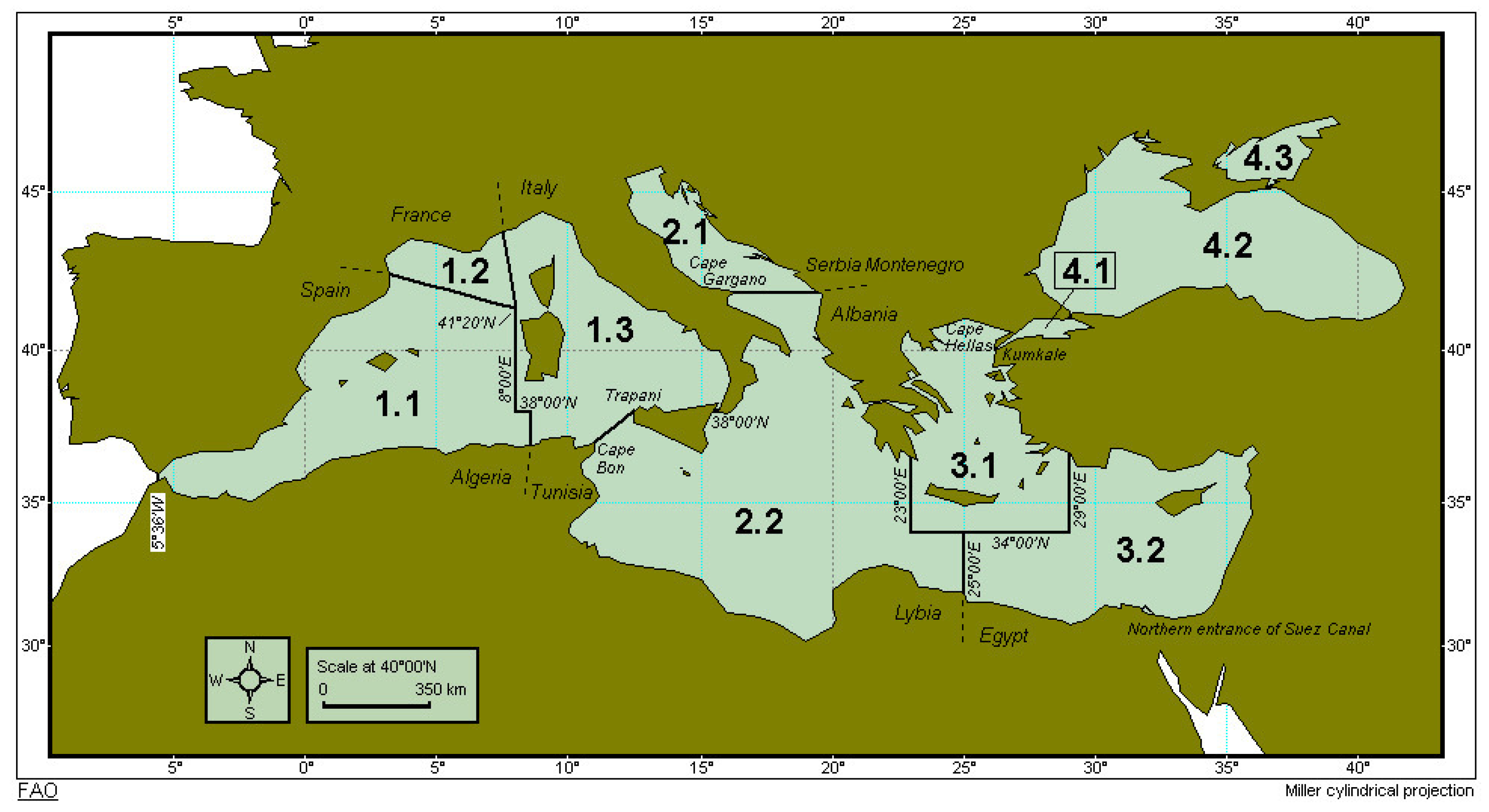
| FAO | Food and Agriculture Organization of the United Nations |
| NPP | Nuclear Power Plant |
| WW | Wet Weight |
References
- Prandle, D. A modelling study of the mixing of 137 Cs in the seas of the European Continental Shelf. Philos. Trans. R. Soc. Lond. Ser. 1984, A310, 407–436. [Google Scholar]
- Breton, M.; Salomon, J.C. A 2d long-term advection–dispersion model for the Channel and southern North-Sea. A: Validation through comparison with artificial radionuclides. J. Mar. Syst. 1995, 6, 495–513. [Google Scholar] [CrossRef]
- Harms, I.; Karcher, M.J.; Dethleff, D. Modelling Siberian river runoff – implications for contaminant transport in the Arctic Ocean. J. Mar. Syst. 2000, 27, 95–115. [Google Scholar] [CrossRef][Green Version]
- Sánchez–Cabeza, J.A.; Ortega, M.; Merino, J.; Masqué, P. Long-term box modelling of 137Cs in the Mediterranean Sea. J. Mar. Syst. 2002, 33, 457–472. [Google Scholar] [CrossRef]
- Kawamura, H.; Kobayashi, T.; Furuno, A.; In, T.; Ishikawa, Y.; Nakayama, T.; Shima, S.; Awaji, T. Preliminary numerical experiments on oceanic dispersion of 131I and 137Cs discharged into the ocean because of the Fukushima Daiichi nuclear power plant disaster. J. Nucl. Sci. Technol. 2011, 48, 1349–1356. [Google Scholar] [CrossRef]
- Behrens, E.; Schwarzkopf, F.U.; Lubbecke, J.; Boning, C.W. Model simulations on the long-term dispersal of 137Cs released into the Pacific Ocean off Fukushima. Environ. Res. Lett. 2012, 7, 034000. [Google Scholar] [CrossRef]
- Tsumune, D.; Tsubono, T.; Aoyama, M.; Hirose, K. Distribution of oceanic 137Cs from the Fukushima Daiichi nuclear power plant simulated numerically by a regional ocean model. J. Environ. Radioact. 2012, 111, 100–108. [Google Scholar] [CrossRef] [PubMed]
- Dvorzhak, A.; Puras, C.; Montero, M.; Mora, J.C. Spanish experience on modeling of environmental radioactive contamination due to Fukushima Daiichi NPP accident using JRODOS. Environ. Sci. Technol. 2012, 46, 11887–11895. [Google Scholar] [CrossRef]
- Masumoto, Y.; Miyazawa, Y.; Tsumune, D.; Kobayashi, T.; Estournel, C.; Marsaleix, P.; Lanerolle, L.; Mehra, A.; Garraffo, Z.D. Oceanic dispersion simulation of Cesium-137 from Fukushima Dai-ichi nuclear power plant. Elements 2012, 8, 207–212. [Google Scholar] [CrossRef]
- Periáñez, R. Models for predicting the transport of radionuclides in the Red Sea. J. Environ. Radioact. 2020, 223–224, 106396. [Google Scholar] [CrossRef]
- Periáñez, R. APERTRACK: A particle-tracking model to simulate radionuclide transport in the Arabian/Persian Gulf. Progr. Nucl. Energ. 2021, 142, 103998. [Google Scholar] [CrossRef]
- Periáñez, R. A Lagrangian tool for simulating the transport of chemical pollutants in the Arabian/Persian Gulf. Modelling 2021, 2, 675–685. [Google Scholar] [CrossRef]
- Maderich, V.; Bezhenar, R.; Kovalets, I.; Khalchenkov, O.; Brovchenko, I. Long–Term Contamination of the Arabian Gulf as a Result of Hypothetical Nuclear Power Plant Accidents. J. Mar. Sci. Eng. 2023, 11, 331. [Google Scholar] [CrossRef]
- Periáñez, R.; Min, B.-I.; Suh, K.-S. The transport, effective half-lives and age distributions of radioactive releases in the northern Indian Ocean. Mar. Pollut. Bull. 2021, 169, 112587. [Google Scholar] [CrossRef] [PubMed]
- Tsabaris, C.; Tsiaras, K.; Eleftheriou, G.; Triantafyllou, G. 137Cs ocean distribution and fate at East Mediterranean Sea in case of a nuclear accident in Akkuyu Nuclear Power Plant. Progr. Nucl. Energ. 2021, 139, 103879. [Google Scholar] [CrossRef]
- Tsabaris, C.; Eleftheriou, G.; Tsiaras, K.; Triantafyllou, G. Distribution of dissolved 137Cs, 131I and 238Pu at eastern Mediterranean Sea in case of hypothetical accident at the Akkuyu nuclear power plant. J. Environ. Radioact. 2022, 251–252, 106964. [Google Scholar] [CrossRef] [PubMed]
- Periáñez, R.; Cortés, C. A Numerical model to simulate the transport of radionuclides in the Western Mediterranean after a nuclear accident. J. Mar. Sci. Eng. 2023, 11, 169. [Google Scholar] [CrossRef]
- Periáñez, R.; Bezhenar, I.; Brovchenko, C.; Duffa, M.; Iosjpe, K.T.; Jung, T.; Kobayashi, F.; Lamego, V.; Maderich, B.I.; Min, H.; et al. Modelling of marine radionuclide dispersion in IAEA MODARIA program: Lessons learnt from the Baltic Sea and Fukushima scenarios. Sci. Total Environ. 2016, 569–570, 594–602. [Google Scholar] [CrossRef]
- IAEA. Modelling of Marine Dispersion and Transfer of Radionuclides Accidentally Released from Land Based Facilities; IAEA–TECDOC–1876; IAEA: Vienna, Austria, 2019. [Google Scholar]
- Periáñez, R.; Bezhenar, R.; Brovchenko, I.; Duffa, C.; Iosjpe, M.; Jung, K.T.; Kobayashi, T.; Liptak, L.; Little, A.; Maderich, V.; et al. Marine radionuclide transport modelling: Recent developments, problems and challenges. Environ. Modell. Softw. 2019, 122, 104523. [Google Scholar] [CrossRef]
- Schonfeld, W. Numerical simulation of the dispersion of artificial radionuclides in the English Channel and the North Sea. J. Mar. Syst. 1995, 6, 529–544. [Google Scholar] [CrossRef]
- Nakano, H.; Motoi, T.; Hirose, K.; Aoyama, M. Analysis of 137Cs concentration in the Pacific using a Lagrangian approach. J. Geophys. Res. 2010, 115, C06015. [Google Scholar]
- Periáñez, R.; Bezhenar, R.; Brovchenko, I.; Jung, K.T.; Kamidara, Y.; Kim, K.O.; Kobayashi, T.; Liptak, L.; Maderich, V.; Min, B.I.; et al. Fukushima 137Cs releases dispersion modelling over the Pacific Ocean. Comparisons of models with water, sediment and biota data. J. Environ. Radioact. 2019, 198, 50–63. [Google Scholar] [CrossRef] [PubMed]
- Bezhenar, R.; Heling, R.; Ievdin, I.; Iosjpe, M.; Maderich, V.; Willemsen, S.; de With, G.; Dvorzhak, A. Integration of marine food chain model POSEIDON in JRODOS and testing versus Fukushima data. Radioprotection 2016, 51, S137–S139. [Google Scholar] [CrossRef]
- Periáñez, R.; Qiao, F.; Zhao, C.; de With, G.; Jung, K.-T.; Sangmanee, C.; Wang, G.; Xia, C.; Zhang, M. Opening Fukushima floodgates: Modelling 137Cs impact in marine biota. Mar. Pollut. Bull. 2021, 170, 112645. [Google Scholar] [CrossRef] [PubMed]
- Bezhenar, R.; Jung, K.T.; Maderich, V.; Willemsen, S.; de With, G.; Qiao, F. Transfer of radiocaesium from contaminated bottom sediments to marine organisms through benthic food chains in post–Fukushima and post–Chernobyl periods. Biogeosciences 2016, 13, 3021–3034. [Google Scholar] [CrossRef]
- Bezhenar, R.; Kim, K.O.; Maderich, V.; de With, G.; Jung, K.T. Multi–compartment kinetic–allometric (MCKA) model of radionuclide bioaccumulation in marine fish. Biogeosciences 2021, 18, 2591–2607. [Google Scholar] [CrossRef]
- Maderich, V.; Bezhenar, R.; Heling, R.; de With, G.; Jung, K.T.; Myoung, J.G.; Cho, Y.K.; Qiao, F.; Robertson, L. Regional long–term model of radioactivity dispersion and fate in the Northwestern Pacific and adjacent seas: Application to the Fukushima Dai–ichi accident. J. Environ. Radioact. 2014, 131, 4–18. [Google Scholar] [CrossRef]
- Maderich, V.; Jung, K.T.; Bezhenar, R.; de With, G.; Qiao, F.; Casacuberta, N.; Masque, P.; Kim, Y.H. Dispersion and fate of 90Sr in the Northwestern Pacific and adjacent seas: Global fallout and the Fukushima Dai–ichi accident. Sci. Total Environ. 2014, 494–495, 261–271. [Google Scholar] [CrossRef]
- Maderich, V.; Bezhenar, R.; Tateda, Y.; Aoyama, M.; Tsumune, D.; Jung, K.T.; de With, G. The POSEIDON–R compartment model for the prediction of transport and fate of radionuclides in the marine environment. MethodsX 2018, 5, 1251–1266. [Google Scholar] [CrossRef]
- De With, G.; Bezhenar, R.; Maderich, V.; Yevdin, Y.; Iosjpe, M.; Jung, K.T.; Qiao, F.; Periáñez, R. Development of a dynamic food chain model for assessment of the radiological impact from radioactive releases to the aquatic environment. J. Environ. Radioact. 2021, 233, 106615. [Google Scholar] [CrossRef]
- Bleck, R. An oceanic general circulation model framed in hybrid isopycnic–Cartesian coordinates. Ocean Model. 2001, 4, 55–88. [Google Scholar] [CrossRef]
- Xu, X.; Chassignet, E.P.; Price, J.F.; Özgökmen, T.M.; Peters, H. A regional modeling study of the entraining Mediterranean outflow. J. Geophys. Res. 2007, 112, C12005. [Google Scholar] [CrossRef]
- Kara, A.B.; Wallcraft, A.J.; Martin, P.J.; Pauley, R.L. Optimizing surface winds using QuikSCAT measurements in the Mediterranean Sea during 2000–2006. J. Mar. Syst. 2009, 78, S119–S131. [Google Scholar] [CrossRef]
- IAEA. Sediment Distribution Coefficients and Concentration Factors for Biota in the Marine Environment; Technical Reports Series 422; IAEA: Vienna, Austria, 2004. [Google Scholar]
- Nyffeler, U.P.; Li, Y.H.; Santschi, P.H. A kinetic approach to describe trace element distribution between particles and solution in natural aquatic systems. Geochim. Cosmochim. Acta 1984, 48, 1513–1522. [Google Scholar] [CrossRef]
- Periáñez, R.; Brovchenko, I.; Duffa, C.; Jung, K.T.; Kobayashi, T.; Lamego, F.; Maderich, V.; Min, B.I.; Nies, H.; Osvath, I.; et al. A new comparison of marine dispersion model performances for Fukushima Dai–ichi releases in the frame of IAEA MODARIA program. J. Environ. Radioact. 2015, 150, 247–269. [Google Scholar] [CrossRef]
- Periáñez, R.; Suh, K.S.; Min, B.I.; Villa, M. The behaviour of 236U in the North Atlantic Ocean assessed from numerical modelling: A new evaluation of the input function into the Arctic. Sci. Total Environ. 2018, 626, 255–263. [Google Scholar] [CrossRef]
- Periáñez, R.; Suh, K.S.; Min, B.I. The behaviour of 137Cs in the North Atlantic Ocean assessed from numerical modelling: Releases from nuclear fuel reprocessing factories, redissolution from contaminated sediments and leakage from dumped nuclear wastes. Mar. Pollut. Bull. 2016, 113, 343–361. [Google Scholar] [CrossRef]
- Periáñez, R.; Bezhenar, R.; Iosjpe, M.; Maderich, V.; Nies, H.; Osvath, I. Outola, I.; de With G. A comparison of marine radionuclide dispersion models for the Baltic Sea in the frame of IAEA MODARIA program. J. Environ. Radioact. 2015, 139, 66–77. [Google Scholar] [CrossRef]
- Kobayashi, T.; Nagai, H.; Chino, M.; Kawamura, H. Source term estimation of atmospheric release due to the Fukushima Dai–ichi Nuclear Power Plant accident by atmospheric and oceanic dispersion simulations. J. Nucl. Sci. Technol. 2013, 50, 255–264. [Google Scholar] [CrossRef]
- Christoudias, T.; Lelieveld, J. Modelling the global atmospheric transport and deposition of radionuclides from the Fukushima Dai–ichi nuclear accident. Atmos. Chem. Phys. 2013, 13, 1425–1438. [Google Scholar] [CrossRef]
- IAEA MARIS. Marine Radioactivity Information System; Division of IAEA Environment Laboratories: Monaco, 2023; Available online: https://maris.iaea.org (accessed on 30 April 2023).
- Uddin, S.; Fowler, S.W.; Behbehani, M.; Al–Ghadban, A.N.; Swarzenski, P.W.; Al–Awadhi, N. A review of radioactivity in the Gulf region. Mar. Pollut. Bull. 2020, 159, 111481. [Google Scholar] [CrossRef] [PubMed]
- Vives i Batlle, J.; Beresford, N.; Beaugelin–Seiller, K.; Bezhenar, R.; Brown, J.; Cheng, J.-J.; Cujic, M.; Dragovic, S.; Duffa, C.; Fievet, B.; et al. Inter-comparison of dynamic models for radionuclide transfer to marine biota in a Fukushima accident scenario. J. Environ. Radioact. 2016, 153, 31–50. [Google Scholar] [CrossRef] [PubMed]
- Periáñez, R. Viewpoint on the Integration of Geochemical Processes into Tracer Transport Models for the Marine Environment. Geosciences 2022, 12, 152. [Google Scholar] [CrossRef]
- Periáñez, R.; Suh, K.S.; Min, B.I.; Casacuberta, N.; Masqué, P. Numerical modelling of the releases of 90Sr from Fukushima to the ocean: An evaluation of the source term. Environ. Sci. Technol. 2013, 47, 12305–12313. [Google Scholar] [CrossRef]
- Sartandel, S.J.; Jha, S.K.; Tripathi, R.M. Latitudinal variation and residence time of 137Cs in Indian coastal environment. Mar. Pollut. Bull. 2015, 100, 489–494. [Google Scholar] [CrossRef] [PubMed]
- Zinger, I.; Oughton, D.H.; Jones, S.R. Stakeholder interaction within the ERICA Integrated Approach. J. Environ. Radioact. 2008, 99, 1503–1509. [Google Scholar] [CrossRef]


| Sr (Target Tissue: Bone) | Cs (Target Tissue: Flesh) | |
|---|---|---|
| Organ fraction f | 0.12 | 0.80 |
| prey (days) | 128 | 75 |
| predator (days) | 257 | 200 |
Disclaimer/Publisher’s Note: The statements, opinions and data contained in all publications are solely those of the individual author(s) and contributor(s) and not of MDPI and/or the editor(s). MDPI and/or the editor(s) disclaim responsibility for any injury to people or property resulting from any ideas, methods, instructions or products referred to in the content. |
© 2023 by the authors. Licensee MDPI, Basel, Switzerland. This article is an open access article distributed under the terms and conditions of the Creative Commons Attribution (CC BY) license (https://creativecommons.org/licenses/by/4.0/).
Share and Cite
Periáñez, R.; Cortés, C. A Study on the Transport of 137Cs and 90Sr in Marine Biota in a Hypothetical Scenario of a Nuclear Accident in the Western Mediterranean Sea. J. Mar. Sci. Eng. 2023, 11, 1707. https://doi.org/10.3390/jmse11091707
Periáñez R, Cortés C. A Study on the Transport of 137Cs and 90Sr in Marine Biota in a Hypothetical Scenario of a Nuclear Accident in the Western Mediterranean Sea. Journal of Marine Science and Engineering. 2023; 11(9):1707. https://doi.org/10.3390/jmse11091707
Chicago/Turabian StylePeriáñez, Raúl, and Carmen Cortés. 2023. "A Study on the Transport of 137Cs and 90Sr in Marine Biota in a Hypothetical Scenario of a Nuclear Accident in the Western Mediterranean Sea" Journal of Marine Science and Engineering 11, no. 9: 1707. https://doi.org/10.3390/jmse11091707
APA StylePeriáñez, R., & Cortés, C. (2023). A Study on the Transport of 137Cs and 90Sr in Marine Biota in a Hypothetical Scenario of a Nuclear Accident in the Western Mediterranean Sea. Journal of Marine Science and Engineering, 11(9), 1707. https://doi.org/10.3390/jmse11091707