
Machine Learning Approach for Detection of Water Overgrowth in Azov Sea with Sentinel-2 Data

 ,
,  ,
,  and
and
Abstract
1. Introduction
- Phragmites australis—86,000 ha;
- Potamogeton—58,000 ha;
- Charophyta—5000 ha;
- Myriophyllum spicatum—4400 ha;
- Scirpus litoralis—3500 ha.
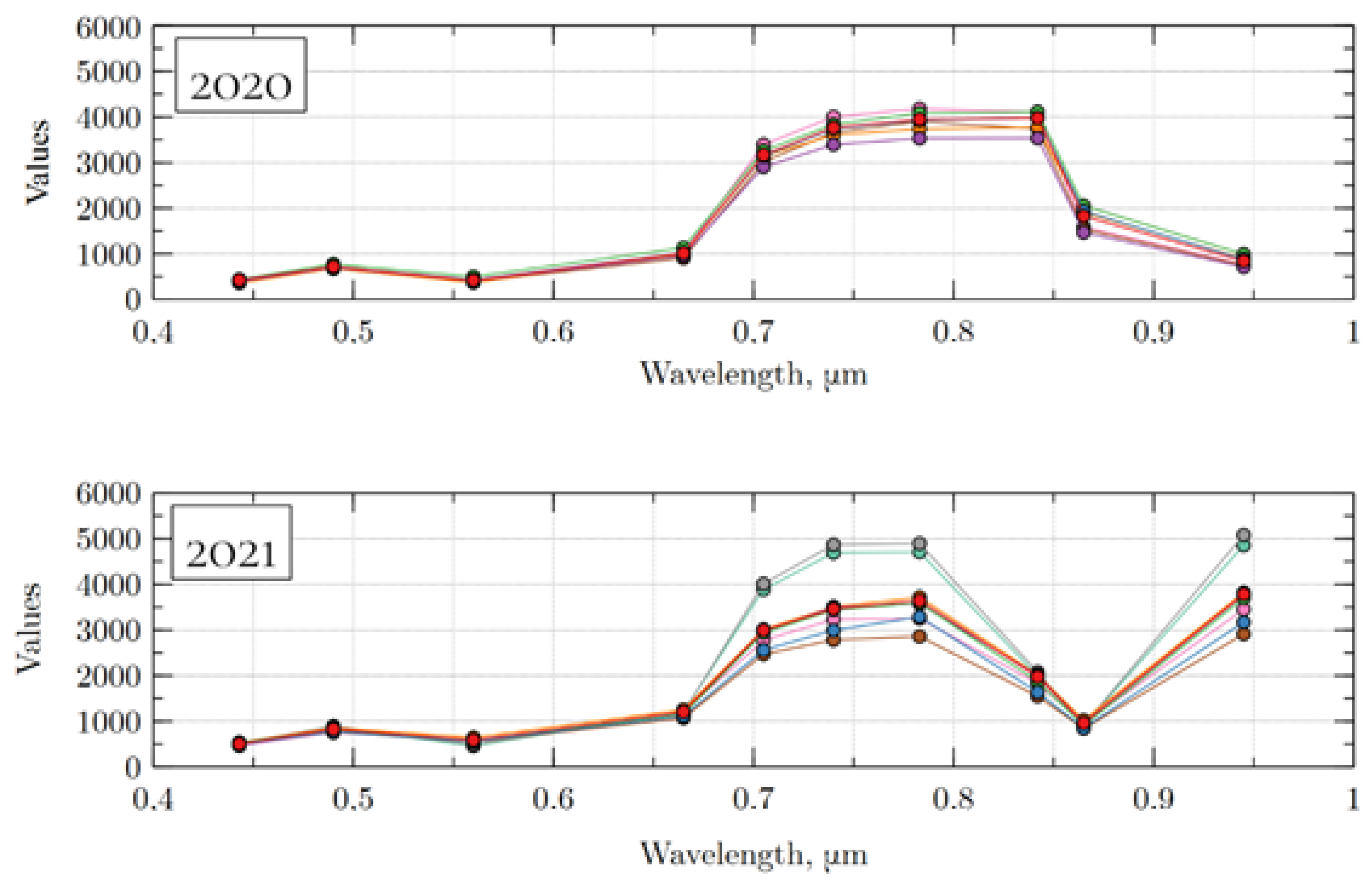
- Shallow parts of the water bodies that are free from vegetation usually formed near the shoreline and deciphered in summer with maximum reflectance values about ≤450, 590–630 μm and 600–630 μm;
- Underwater vegetation was detected in summer using remote sensing data with maximum reflectance in the near-infrared (NIR) band and near 710 μm.
2. Previous Work
- 0 class—from −1.0 to −0.1 (open surfaces, free from vegetation);
- 1 class—from −0.1 to 0.3 (hydrophytes located below the water surface);
- 2 class—from 0.3 to 0.5 (hydrophytes located on the water surface);
- 3 class—from 0.5 to 1.0 (emergent vegetation).
3. Materials and Methods
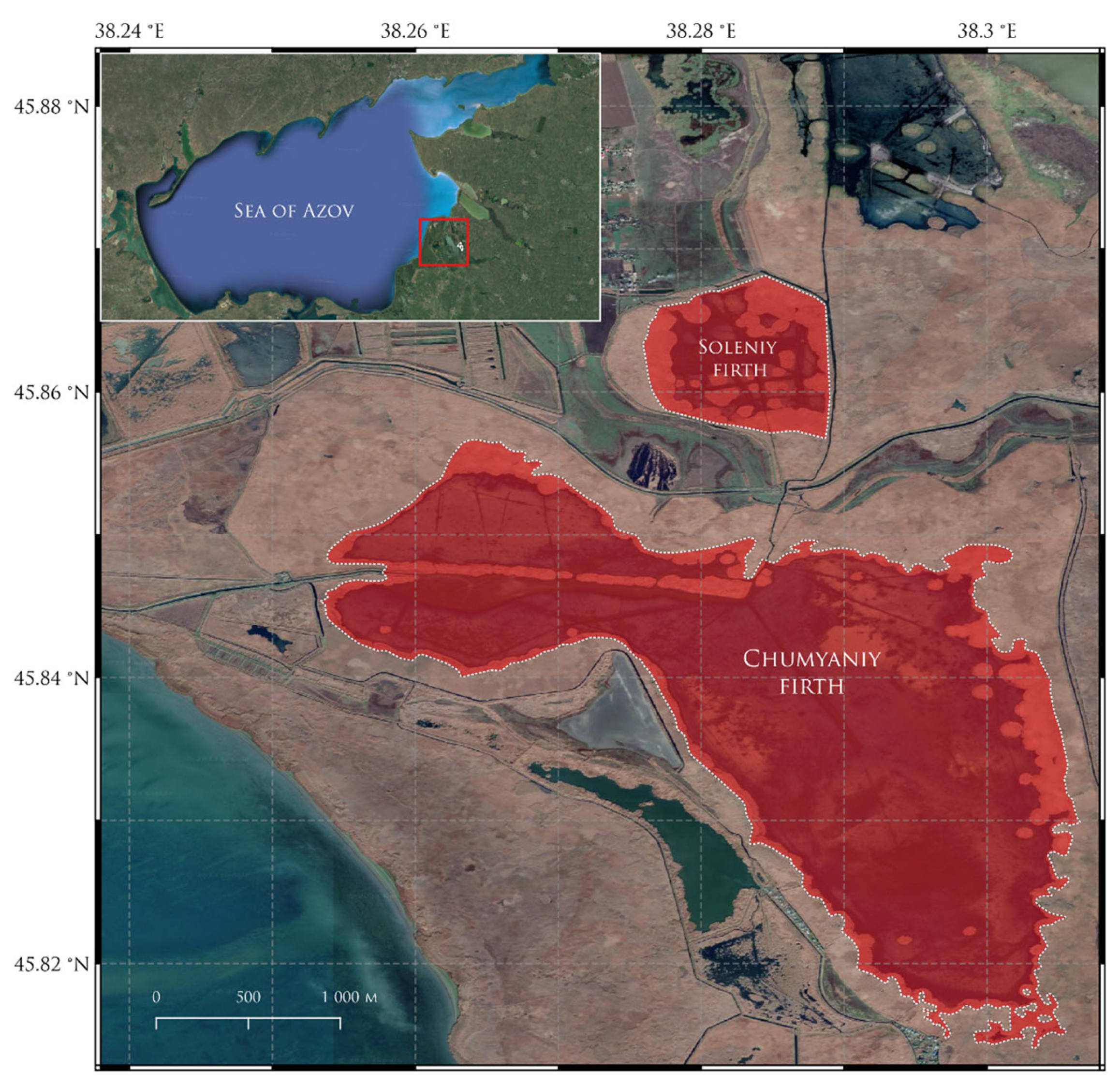
3.1. Research Area
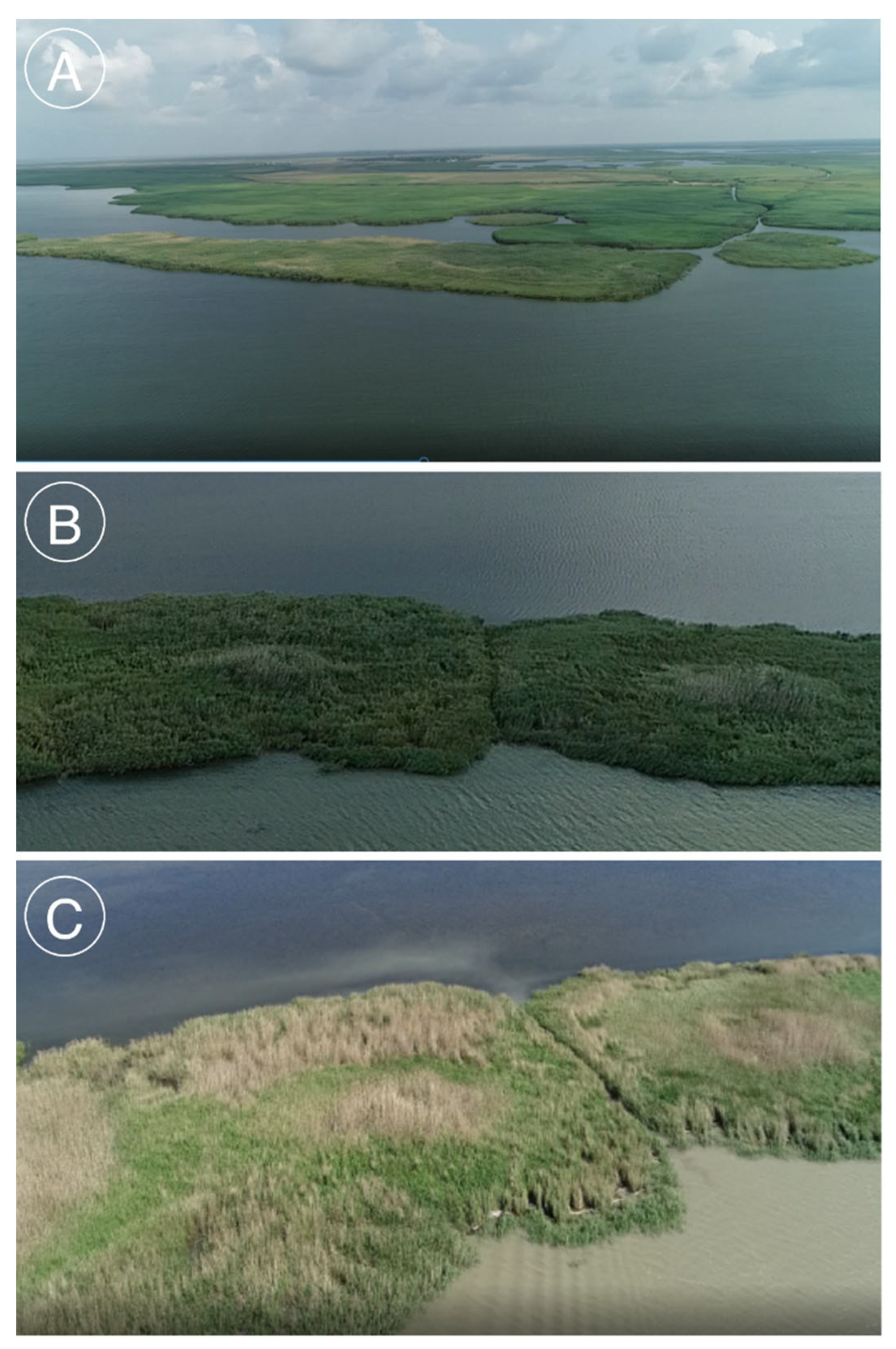
3.2. Field Data Collection
3.3. Remote Sensing Data
3.4. Spectral Signatures Extraction
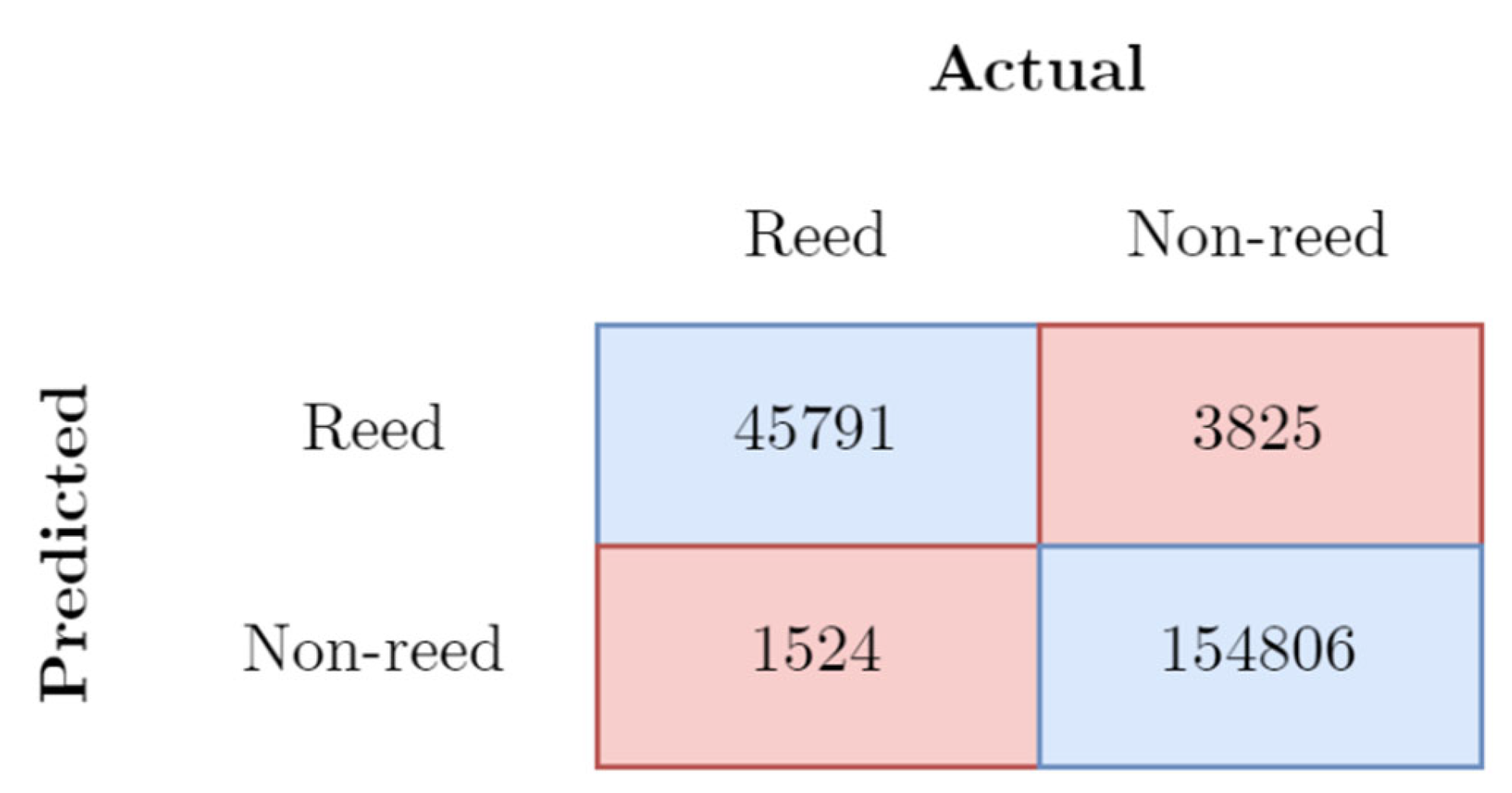
3.5. Accuracy Assessment
3.6. Reed Classification
4. Results and Discussion
- Phragmites can outcompete native vegetation and alter the composition and structure of wetland ecosystems, which can have a cascading effect on other species that depend on those habitats. The invasive species can form dense, monotypic stands that displace native vegetation, leading to the loss of biodiversity and changing the functional dynamics of the ecosystem.
- The invasion of Phragmites can lead to a decline in native plant and animal species, reducing biodiversity in affected areas. The displacement of native vegetation can reduce the habitat quality and availability of many species, including those that are threatened or endangered.
- Phragmites can change the hydrology of wetland ecosystems, leading to soil degradation and potentially altering water quality. The species has a deep root system that can affect soil stability and water flow, leading to changes in the ecosystem’s hydrological cycle and increasing the risk of erosion and sedimentation.
- The dense stands of Phragmites can increase the risk of fire, which can further alter wetland ecosystems. This can have a direct impact on the vegetation and wildlife of the area, altering the structure and composition of the ecosystem.
- Wetlands, including those dominated by Phragmites, can play an important role in carbon sequestration, but the rapid growth of Phragmites can alter the balance of carbon in wetland ecosystems. The species can significantly impact the carbon storage potential of wetland ecosystems, which can have wider implications for global climate change.
5. Conclusions
Author Contributions
Funding
Data Availability Statement
Conflicts of Interest
References
- Mikhailova, K.B.; Mikhalap, S.G. Spawning Grounds Overgrowth Dynamics of the Pskov Lake on Anokhov Bay Example. Ecosyst. Transform. 2020, 1, 83–94. [Google Scholar]
- Tsunikova, E.P. Water Bodies of the Eastern Azov Region: Their Fishery Significance and Optimization of Their Practical Use; Mediapolis Publishing: Moscow, Russia, 2006. [Google Scholar]
- Matishov, G.G.; Matishov, D.G.; Namjatov, A.A.; Carroll, J.; Dahle, S. Artificial Radionuclides in Sediments of the Don River Estuary and Azov Sea. J. Environ. Radioact. 2002, 59, 309–327. [Google Scholar] [CrossRef] [PubMed]
- Moses, W.J.; Gitelson, A.A.; Berdnikov, S.; Povazhnyy, V. Satellite Estimation of Chlorophyll-$a$ Concentration Using the Red and NIR Bands of MERIS—The Azov Sea Case Study. IEEE Geosci. Remote Sens. Lett. 2009, 6, 845–849. [Google Scholar] [CrossRef]
- Mosesyan, G.; Dudkin, S.; Strizhakova, T. Assessment of infection of Hamsa Engraulis encrasicolus nematode Hysterothylacium aduncum in the Sea of Azov in the summer and autumn periods 2015–2020. Fisheries 2021, 2021, 25–30. [Google Scholar] [CrossRef]
- Nabozhenko, M.V.; Kovalenko, E.P. Contemporary Distribution of Macrozoobenthic Communities of the Yeisk Estuary (Taganrog Bay of the Sea of Azov). Oceanology 2011, 51, 626. [Google Scholar] [CrossRef]
- Shekhov, A.G. Flora and Vegetation of Kuban Estuaries. Inland Water Biol. 1971, 10, 24–29. [Google Scholar]
- Shekhov, A.G. Influence of Watering Timing and Overgrowing of Fish Ponds in the Don Delta. Bot. Zhurnal 1970, 55, 1152–1157. [Google Scholar]
- Bondarenko, L.G.; Kulba, S.N.; Petrashov, V.I.; Smirnov, S.S.; Matveeva, E.I.; Rudakova, N.A. Assessment of Overgrowth of the Chelbas Group of the Azov Sea Limans with Aquatic Vegetation. Water Bioresour. Environ. 2021, 4, 14–26. [Google Scholar] [CrossRef]
- Borovskaya, R.; Krivoguz, D.; Chernyi, S.; Kozhurin, E.; Zinchenko, E. Surface Water Salinity Evaluation and Identification for Using Remote Sensing Data and Machine Learning Approach. J. Mar. Sci. Eng. 2022, 10, 257. [Google Scholar] [CrossRef]
- Antonenko, M.V.; Fedorova, S.I. Satellite Monitoring of the Kulikov-Kurchansk Group of Limans. Innov. Sci. 2016, 3, 59–61. [Google Scholar]
- Filonenko, I.V.; Komarova, A.S. Long-Term Dynamics of the Area Overgrown with Coastal Aquatic Vegetation of Lake Vozhe. Printsipy Ekol. 2015, 16, 63. [Google Scholar] [CrossRef]
- Kochetkova, A.I.; Bryzgalina, E.S.; Kalyuzhnaya, I.Y.; Sirotina, S.L.; Samoteyeva, V.V.; Rakshenko, E.P. Overgrowth Dynamics of the Tsimlyanskoe Reservoir. Princ. Ecol. 2018, 26, 60–72. [Google Scholar] [CrossRef]
- Vlasov, B.P.; Hryshchankava, N.D.; Sivenkou, A.Y.; Sukhovilo, N.Y.; Kolbun, D.A. Assessment of the Current State and Dynamics of the Overgrowing of Lakes in National Park “Narochansky” Using Remote Sensing Data. Acta Geogr. Sil. 2019, 13, 39–55. [Google Scholar]
- Peng, J.; Liu, S.; Lu, W.; Liu, M.; Feng, S.; Cong, P. Continuous Change Mapping to Understand Wetland Quantity and Quality Evolution and Driving Forces: A Case Study in the Liao River Estuary from 1986 to 2018. Remote Sens. 2021, 13, 4900. [Google Scholar] [CrossRef]
- Lamb, B.T.; Tzortziou, M.A.; McDonald, K.C. A Fused Radar–Optical Approach for Mapping Wetlands and Deepwaters of the Mid–Atlantic and Gulf Coast Regions of the United States. Remote Sens. 2021, 13, 2495. [Google Scholar] [CrossRef]
- Oteman, B.; Scrieciu, A.; Bouma, T.J.; Stanica, A.; van der Wal, D. Indicators of Expansion and Retreat of Phragmites Based on Optical and Radar Satellite Remote Sensing: A Case Study on the Danube Delta. Wetlands 2021, 41, 72. [Google Scholar] [CrossRef]
- Krivoguz, D.; Mal’ko, S.; Borovskaya, R.; Semenova, A. Automatic Processing of Sentinel-2 Image for Kerch Peninsula Lake Areas Extraction Using QGIS and Python. E3S Web Conf. 2020, 203, 3011. [Google Scholar] [CrossRef]
- Krivoguz, D.; Bespalova, L.; Zhilenkov, A.; Chernyi, S. A Deep Neural Network Method for Water Areas Extraction Using Remote Sensing Data. J. Mar. Sci. Eng. 2022, 10, 1392. [Google Scholar] [CrossRef]
- Bondarenko, L.G.; Kulba, S.N.; Petrashov, V.I.; Smirnov, S.S.; Matveeva, E.I. The influence of changes in the hydrological parameters of limans of the Eastern-Akhtarsky growing farm with the overgrowth of hydrophytes. Bull. KSMTU 2022, 3, 24–39. [Google Scholar]
- Papchnkov, V.G.; Scherbakov, A.V.; Lapirov, A.G. Main Hydrobotanical Definitions and Terms. In Proceedings of the Hydrobotany: Methodology, Methods, Moscow, Russia, 19 May 2003; pp. 27–38. [Google Scholar]
- Lapirov, A.G. Ecological Groups of Aquatic Vegetation. In Proceedings of the Hydrobotany: Methodology, Methods, Moscow, Russia, 19 May 2003; pp. 5–22. [Google Scholar]
- Zernov, A.S. Illustrated Flora of the Russian Black Sea South Region; KMK: Rostov, Russia, 2013. [Google Scholar]
- Gollerbach, M.M.; Kosinskaya, E.K.; Polyanskiy, V.I. Qualifier of Freshwater Algae in USSR; Soviet Science: Moscow, Russia, 1953. [Google Scholar]
- Joshi, S.; Rai, N.; Sharma, R.; Baral, N. Land Use/Land Cover (LULC) Change in Suburb of Central Himalayas: A Study from Chandragiri, Kathmandu. J. For. Environ. Sci. 2021, 37, 44–51. [Google Scholar] [CrossRef]
- Krivoguz, D.O.; Burtnik, D.N. Neural Network Modeling of Changes in the Land Cover of the Kerch Peninsula in the Context of Landslides Occurence. Nauchno-Tekhnicheskiy Vestn. Bryanskogo Gos. Univ. 2018, 1, 113–121. [Google Scholar] [CrossRef]
- Souza, J.M.d.; Morgado, P.; Costa, E.M.d.; Vianna, L.F.d.N. Modeling of Land Use and Land Cover (LULC) Change Based on Artificial Neural Networks for the Chapecó River Ecological Corridor, Santa Catarina/Brazil. Sustainability 2022, 14, 4038. [Google Scholar] [CrossRef]
- Thiam, S.; Salas, E.A.L.; Hounguè, N.R.; Almoradie, A.D.S.; Verleysdonk, S.; Adounkpe, J.G.; Komi, K. Modelling Land Use and Land Cover in the Transboundary Mono River Catchment of Togo and Benin Using Markov Chain and Stakeholder’s Perspectives. Sustainability 2022, 14, 4160. [Google Scholar] [CrossRef]
- Congedo, L. Semi-Automatic Classification Plugin: A Python Tool for the Download and Processing of Remote Sensing Images in QGIS. J. Open Source Softw. 2021, 6, 3172. [Google Scholar] [CrossRef]
- Chernyi, S.; Emelianov, V.; Zinchenko, E.; Zinchenko, A.; Tsvetkova, O.; Mishin, A. Application of Artificial Intelligence Technologies for Diagnostics of Production Structures. J. Mar. Sci. Eng. 2022, 10, 259. [Google Scholar] [CrossRef]
- Zhilenkov, A.; Chernyi, S.; Emelianov, V. Application of Artificial Intelligence Technologies to Assess the Quality of Structures. Energies 2021, 14, 8040. [Google Scholar] [CrossRef]
- Breiman, L. Random Forests. Mach. Learn. 2001, 45, 5–32. [Google Scholar] [CrossRef]
- Corcoran, J.M.; Knight, J.F.; Gallant, A.L. Influence of Multi-Source and Multi-Temporal Remotely Sensed and Ancillary Data on the Accuracy of Random Forest Classification of Wetlands in Northern Minnesota. Remote Sens. 2013, 5, 3212–3238. [Google Scholar] [CrossRef]
- Cutler, D.R.; Edwards, T.C., Jr.; Beard, K.H.; Cutler, A.; Hess, K.T.; Gibson, J.; Lawler, J.J. Random Forests for Classification in Ecology. Ecology 2007, 88, 2783–2792. [Google Scholar] [CrossRef]
- Feng, Q.; Gong, J.; Liu, J.; Li, Y. Monitoring Cropland Dynamics of the Yellow River Delta Based on Multi-Temporal Landsat Imagery over 1986 to 2015. Sustainability 2015, 7, 14834–14858. [Google Scholar] [CrossRef]
- Chistiakov, S. Random Forests: An Overview. Trans. KarRC RAS 2013, 12, 117–136. [Google Scholar]


| Band | Wavelength (µm) | Resolution (m) | Purpose |
|---|---|---|---|
| B1 | 443 | 60 | Blue |
| B2 | 490 | 10 | Green |
| B3 | 560 | 10 | Red |
| B4 | 665 | 10 | Red Edge |
| B5 | 705 | 20 | Vegetation Red Edge |
| B6 | 740 | 20 | Vegetation Red Edge |
| B7 | 783 | 20 | Vegetation Red Edge |
| B8A | 842 | 20 | Near Infrared |
| B11 | 1610 | 20 | Shortwave Infrared 1 |
| B12 | 2190 | 20 | Shortwave Infrared 2 |
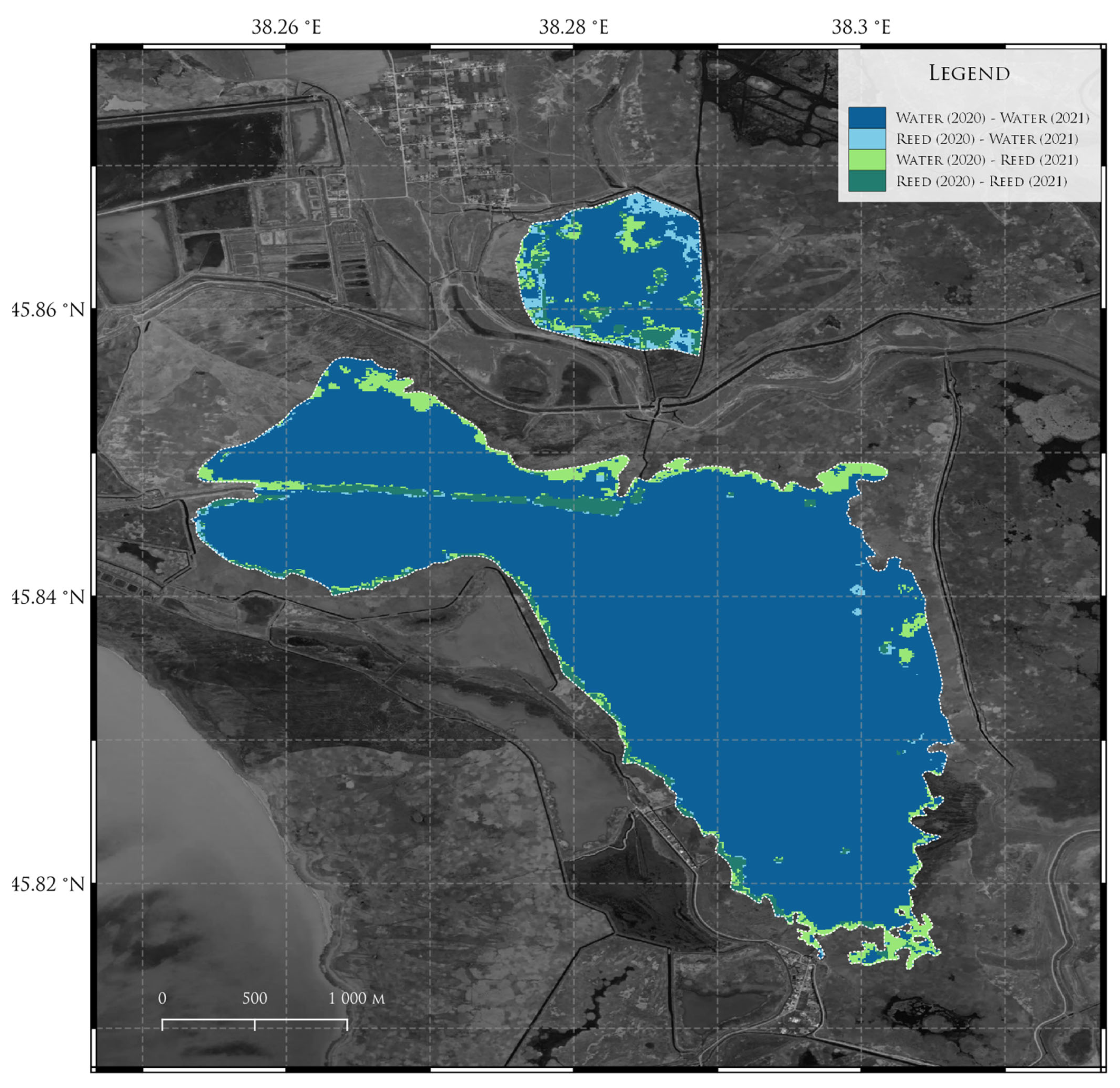
| 2020 | 2021 | Area (km2) |
|---|---|---|
| Water | Water | 7.97 |
| Reed | Water | 0.16 |
| Water | Reed | 0.50 |
| Reed | Reed | 0.37 |
Disclaimer/Publisher’s Note: The statements, opinions and data contained in all publications are solely those of the individual author(s) and contributor(s) and not of MDPI and/or the editor(s). MDPI and/or the editor(s) disclaim responsibility for any injury to people or property resulting from any ideas, methods, instructions or products referred to in the content. |
© 2023 by the authors. Licensee MDPI, Basel, Switzerland. This article is an open access article distributed under the terms and conditions of the Creative Commons Attribution (CC BY) license (https://creativecommons.org/licenses/by/4.0/).
Share and Cite
Krivoguz, D.; Bondarenko, L.; Matveeva, E.; Zhilenkov, A.; Chernyi, S.; Zinchenko, E. Machine Learning Approach for Detection of Water Overgrowth in Azov Sea with Sentinel-2 Data. J. Mar. Sci. Eng. 2023, 11, 423. https://doi.org/10.3390/jmse11020423
Krivoguz D, Bondarenko L, Matveeva E, Zhilenkov A, Chernyi S, Zinchenko E. Machine Learning Approach for Detection of Water Overgrowth in Azov Sea with Sentinel-2 Data. Journal of Marine Science and Engineering. 2023; 11(2):423. https://doi.org/10.3390/jmse11020423
Chicago/Turabian StyleKrivoguz, Denis, Liudmila Bondarenko, Evgenia Matveeva, Anton Zhilenkov, Sergei Chernyi, and Elena Zinchenko. 2023. "Machine Learning Approach for Detection of Water Overgrowth in Azov Sea with Sentinel-2 Data" Journal of Marine Science and Engineering 11, no. 2: 423. https://doi.org/10.3390/jmse11020423
APA StyleKrivoguz, D., Bondarenko, L., Matveeva, E., Zhilenkov, A., Chernyi, S., & Zinchenko, E. (2023). Machine Learning Approach for Detection of Water Overgrowth in Azov Sea with Sentinel-2 Data. Journal of Marine Science and Engineering, 11(2), 423. https://doi.org/10.3390/jmse11020423