Relationship between the Spatial and Temporal Distribution of Squid-Jigging Vessels Operations and Marine Environment in the North Pacific Ocean

Abstract

Information and understanding of fishing activities at sea is important to fisheries science, public authorities and policy-makers. To understand the spatial–temporal distribution characteristics of squid-jigging vessels and how the marine environment affects the distribution of squid-jigging vessels in the North Pacific Ocean, operation behavior of the squid-jigging vessels was analysed by using spatial–temporal factors and marine environmental factors. The fishing effort (FE) information was calculated based on automatic identification system (AIS) data of squid-jigging fishing vessels in the North Pacific Ocean from July to November in 2017 to 2020, and the overlay maps of the spatial distribution of environmental factors and fishing effort were plotted together with four environmental variables (sea surface temperature (SST), sea surface height (SSH), sea surface salinity (SSS), and concentration of chlorophyll-a (Chla)). A generalized additive model (GAM) was used to investigate the nonlinear influence of the marine environment on squid-jigging fishing vessel activity in the North Pacific Ocean. The results show that fishing effort increased from July to August and then decreased from September to November. The fishing effort was highest in August. The intensity of the fishing effort suggests squid-jigging vessel operations had significant seasonal variations. The overlay maps suggest that the fishing effort of squid-jigging vessels was mainly located in areas where SST was between $10{}^{\circ }\mathrm{C}$ and $20{}^{\circ }\mathrm{C}$, SSH was between $-0.3\mathrm{m}$ and $0.2\mathrm{m}$, SSS was between $32\times {10}^{-3}$ and $34\times {10}^{-3}$, and Chla was between $0.1\mathrm{mg}·{\mathrm{m}}^{-3}$ and $0.4\mathrm{mg}·{\mathrm{m}}^{-3}$. The generalized additive model indicated evidence of nonlinear relationships between fishing effort and the three environmental factors. The favorable ranges of SST, SSH, SSS and Chla for fishing effort were $15{}^{\circ }\mathrm{C}\sim 18{}^{\circ }\mathrm{C}$, $0\sim 0.2\mathrm{m}$, $33\times {10}^{-3}\sim 34\times {10}^{-3}$ and $0.2\mathrm{mg}·{\mathrm{m}}^{-3}\sim 0.4\mathrm{mg}·{\mathrm{m}}^{-3}$, respectively. Moreover, the area beneficial to fishing effort was in ${41}^{\circ }\mathrm{N}\sim {44}^{\circ }\mathrm{N}$, ${152}^{\circ }\mathrm{E}\sim {165}^{\circ }\mathrm{E}$.

1. Introduction

The neon flying squid (Ommastrephes bartramii), the main fishing target of squid-jigging vessels in the North Pacific Ocean, is an economically important oceanic cephalopod species [1,2]. O. bartramii is an essential and important component of marine food webs and serves as a predator of numerous small species and a crucial prey species for numerous large marine organisms [3]. Therefore, it is extremely important to understand the spatial–temporal distribution and sustainable utilization of O. bartramii resources for ecosystem protection. The neon flying squid distribution and relative abundance are closely linked to changes in environmental conditions. Numerous studies have found that the potential fishing grounds of O. bartramii in the North Pacific were largely influenced by marine environmental variables such as sea surface temperature (SST), sea surface salinity (SSS), chlorophyll-a concentration (Chla) and sea surface height (SSH) [4,5,6,7,8].

The North Pacific population of O. bartramii is comprised of two seasonal spawning cohorts: the fall and winter–spring spawning cohorts and undergo north–south migration driven by feeding and spawning [8]. The spatial distribution of the two cohorts can been classed into four stocks: the western and central-eastern stocks of the winter–spring cohort; the central and eastern stocks of the autumn cohort [9]. In previous studies, the analysis of fishery conditions was based on single commercial fishing data. A prediction model was established by using the commercial fishing data. Research results were limited in spatio–temporal range relative to potential fishing grounds. The sample selection bias from limitations on spatial coverage also results in environmental bias and could introduce estimation errors in models [5].

The log data adopted in previous studies were historic data due to the time lags, usually several years ago [1,5]. It is well known that O. bartramii distribution and abundance are demonstrably quite different from year to year [6]. There is also significant seasonal variability in habitat quality [7], and the squid vessel fishing location shows obvious difference between months [1,5]. For a 1-year short-lived lifespan species, its spatial–temporal distribution is highly susceptible to changes in marine conditions. It is necessary to adopt not only medium- term and long-term policies, but also flexible, short- and medium-term management policies [10]. Short-term, flexible management policies require continuous and near real-time monitoring of the spatial distribution of the fish. Hence, a comprehensive sampling, near real-time substitutable fishery information is necessary.

Recent developments in large data collected from the Automatic Identification System (AIS) [11,12,13] now provides dynamic vessel information, which was used for vessel safety [14,15,16] and fishing vessel monitoring [17] at first. It is now used for environmental pollution [18,19,20], traffic monitoring [21,22,23] and marine spatial planning [24,25,26,27,28]. The fishing effort information calculated from AIS also show great value in fishery resources. The fishing effort was used to investigate the characteristics of fishing behaviour [29], map high-resolution fishing grounds by detecting the fishing operation location [30] and determine the impact of human fishing activities on marine ecology [31]. The marine environment impacts the spatial–temporal distribution of fishery resources and thereby indirectly impacts the dynamic distribution of fishing spaces. The relationship between the temporal and spatial distribution of fishing vessel operation and marine surface environment has been preliminarily analysed by using ecological models and predicting fishing grounds [32,33,34,35].

Until now, hundreds of scientific research articles have been published regarding the spatial and temporal dynamics of fishing vessels. The squid-jigging vessel fishing location in the North Pacific Ocean shows significant difference between months, and is related to marine environment change. However, the spatial distribution of squid-jigging fishing vessels and its relationship with the marine environment have not been reported. In this study, the fishing effort data calculated from squid-jigging vessel tracking information in the North Pacific Ocean is coupled with remotely-sensed environmental data to analyse the spatial distribution of fishing vessel operation and its relationship with the marine environment, to support the vessels and fishery resource management.

2. Materials and Methods

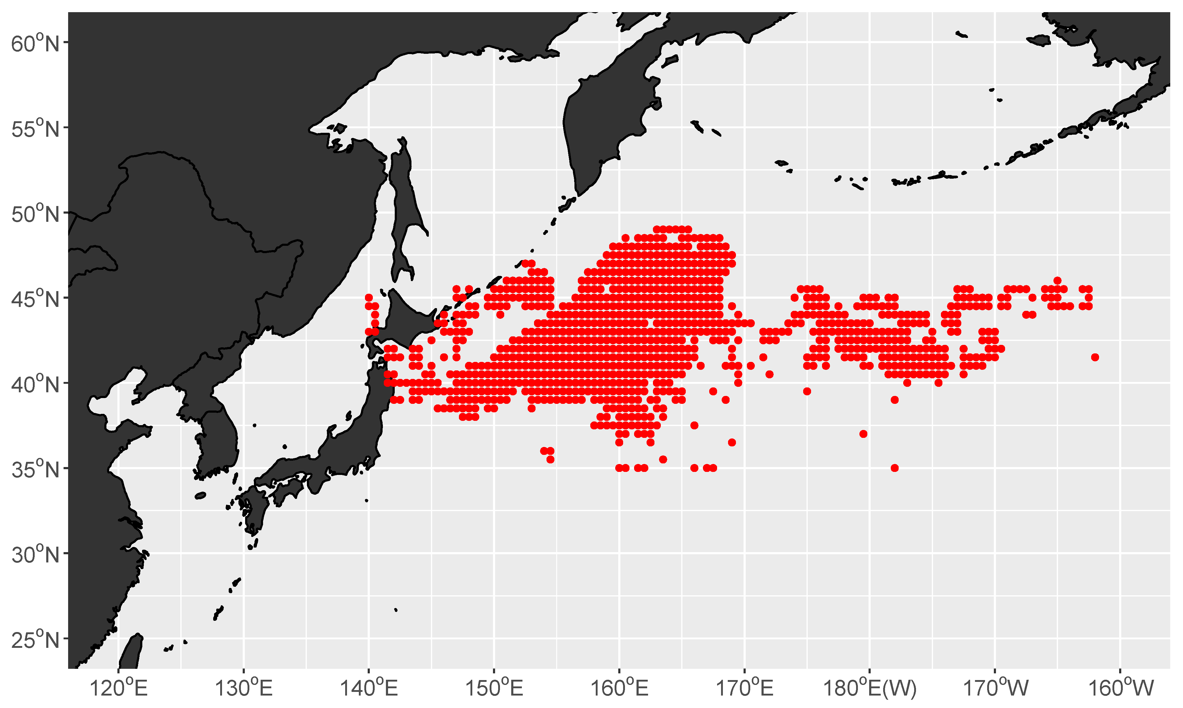
2.1. Study Area

The traditional squid-jigging fishing area is mainly distributed in the western North Pacific (${140}^{\circ }\mathrm{E}\sim {160}^{\circ }\mathrm{W}$, ${35}^{\circ }\mathrm{N}\sim {50}^{\circ }\mathrm{N}$) (Figure 1). In this area, there are two predominant western boundary currents, the warm Kuroshio Current and the cold Oyashio Current [36]. The dynamic and productive ecosystem is mainly influenced by the two currents.

2.2. Fishing Vessel Data Sources and Processing

The fishing effort data of squid-jigging fishing vessels were downloaded from Global Fishing Watch (https://globalfishingwatch.org/, accessed on 8 June 2021). The data included date, latitude, longitude, (Maritime Mobile Service Identify, MMSI), sailing time and fishing time information. The spatial resolution was 0.1 degrees and the temporal resolution was in days. The time was calculated by assigning an amount of time to each AIS detection and then summing those results at all positions in each grid cell. The fishing effort of the squid-jigging fishery was calculated through the convolutional neural network (CNN) [37].

The spatial pattern of the squid-jigging fishing location shows two distinct fishing areas divided by 170${}^{\circ }$ E. The distribution of fishing effort between the western and eastern regions for the squid-jigging fishery from 2012 to 2020 are shown in Figure 2a,b, respectively. The fishing effort increased from 2017. In order to eliminate the spatial sample bias, the data after 2017 were adopted for analysis. According to the migration characteristics of O. bartramii, the fishing season for squid is generally from July and November [6]. Therefore, the time range of the fishing effort data selected in this paper was from July to November. The previous study [38] indicated that the optimal temporal and spatial scales are month, and ${0.5}^{\circ }$ latitude and ${0.5}^{\circ }$ longitude for O. bartramii in the Northwest Pacific Ocean. The fishing effort was compiled to monthly and ${0.5}^{\circ }$ resolution.

2.3. Marine Environmental Data

The important environmental factors impacting the O. bartramii spatial–temporal distribution in the North Pacific Ocean usually include SST, SSH, SSS and Chla [5,39,40]. In this study, SST, SSH, SSS and Chla from July to November 2017–2020 were used to study the relationship between environmental conditions and the spatial distribution of squid-jigging vessels. These environmental data were obtained from the website: https://resources.marine.copernicus.eu/?option=com_csw&task=results, accessed on 8 June 2021. The environmental data were processed to a spatial resolution of ${0.5}^{\circ }\times {0.5}^{\circ }$ and were averaged by month.

2.4. Gravity of Fishing Effort

In this paper, the fishing effort in the grids corresponding from July to November in 2017 to 2019 was averaged by month as the fishing effort of the squid-jigging vessels in this grid. The equation for calculating the gravity of the fishing effort is as follows [41]:

$$X={\displaystyle \frac{{\sum }_{i=1}^n(E_i\times X_i)}{{\sum }_{i=1}^n{E}_i}},Y={\displaystyle \frac{{\sum }_{i=1}^n(E_i\times Y_i)}{{\sum }_{i=1}^n{E}_i}}.$$

(1)

where X and Y are the longitude and latitude of fishing effort center of gravity, respectively; $X_i$ is latitude of central point of the i-th grid; $Y_i$ is longitude of central point of the i-th grid; $E_i$ is the fishing effort in the i-th grid.

2.5. Analysis of the Relationship between Fishing Effort and the Marine Environment

To understand the impacts of the marine environment on the distribution of working areas for squid-jigging vessels, in this study, we developed an overlay map of fishing efforts with SST, SSH, SSS and Chla to visualize the suitable range of marine environmental parameters for fishing efforts. The suitable range of marine environmental parameters for the fishing effort distribution was analyzed by using mathematical statistical methods. We use Matlab2018b to implement this method.

2.6. Generalized Additive Model

In this paper, the generalized additive model (GAM) was used to establish nonlinear response relationships for the fishing effort of squid-jigging vessels, spatial variables, and marine environmental variables. In addition, the nonlinear impacts of spatial variables and marine environmental variables on fishing efforts were analyzed according to the GAM model. The GAM model has been widely used in fishery research [6,39,40]. The spatial variables included longitude and latitude, and the marine environmental variables included SST, SSH, SSS and Chla. Here, the formula of GAM [6,39,40] is as follows:

$$ln(effort+0.1)\sim \mathrm{s}(Lon,Lat)+\mathrm{s}\left(SST\right)+\mathrm{s}\left(SSH\right)+\mathrm{s}\left(SSS\right)+\mathrm{s}\left(Chla\right),$$

(2)

where $\mathrm{s}\left(\right)$ is the natural spline smoothing function and $\mathrm{s}(Lon,Lat)$ represents the influence of spatial factors on the area of fishing vessel operations as the result of the interaction of longitude and latitude. The mgcv function library of the R package was used to construct and calculate the GAM model, and the AIC value was used for model selection. The relation function adopted a Gaussian distribution. The smoothing function adopted the adaptive smoother function based on the P spline, the freedom of the smoothing function was not set, and the optimal function order was chosen by automatic model simulation. The optimal function order was selected by automatic simulation of the model in R language. In addition, To compare the marine environmental impact differences at different spatial scales, four spatial scale GAM models were constructed, which included ${0.1}^{\circ }\times {0.1}^{\circ }$, ${0.25}^{\circ }\times {0.25}^{\circ }$, ${0.5}^{\circ }\times {0.5}^{\circ }$ (excluding latitude and longitude) and $1^{\circ }\times 1^{\circ }$, respectively.

3. Results

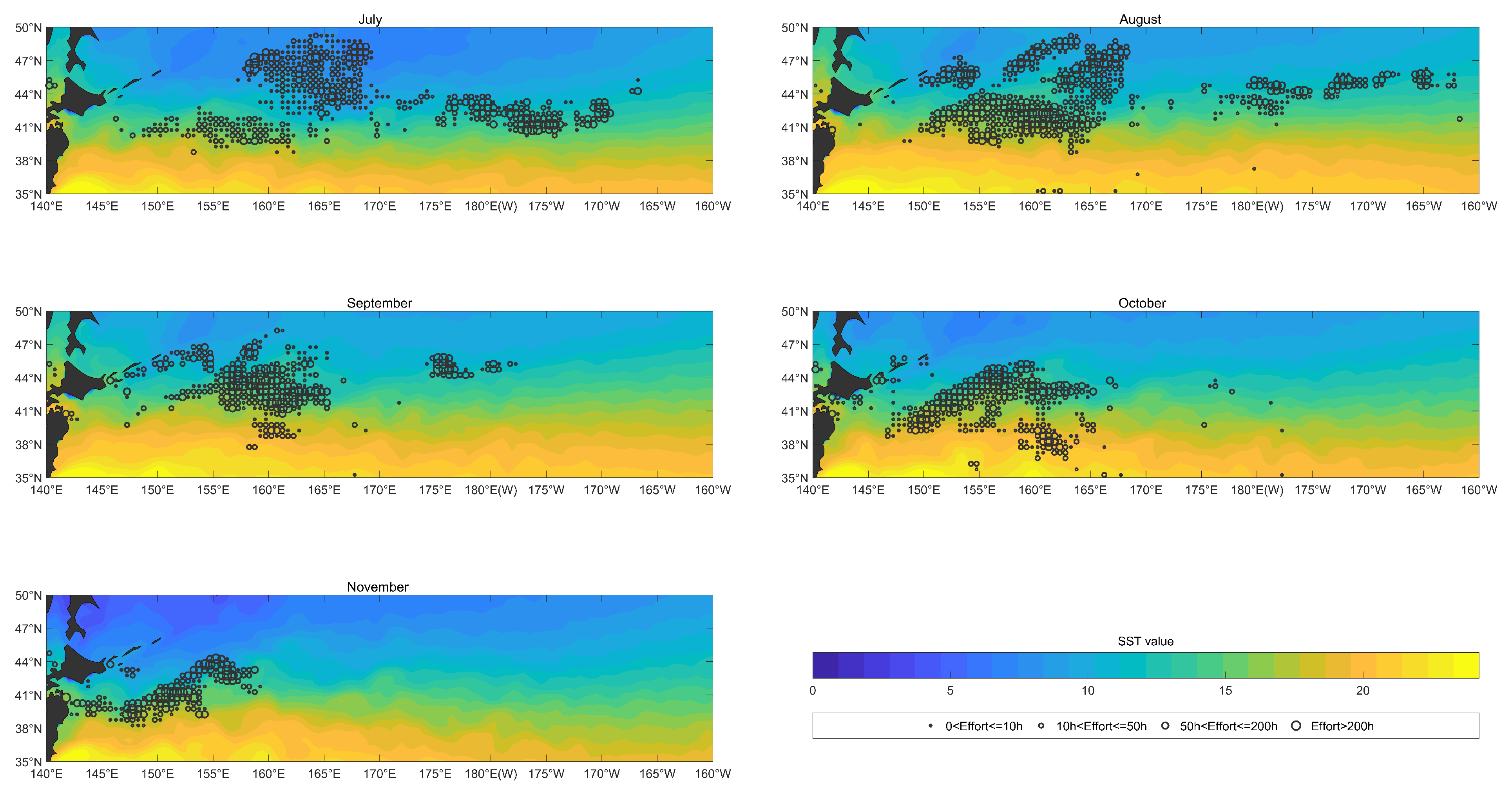
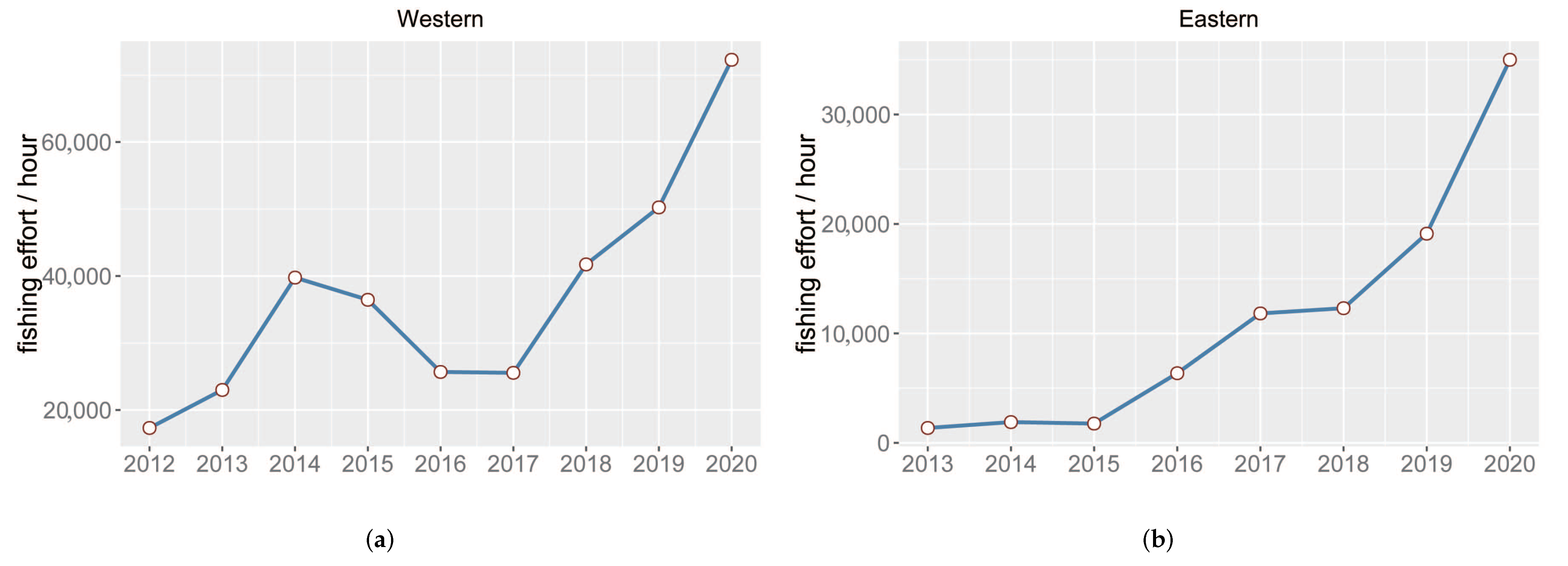
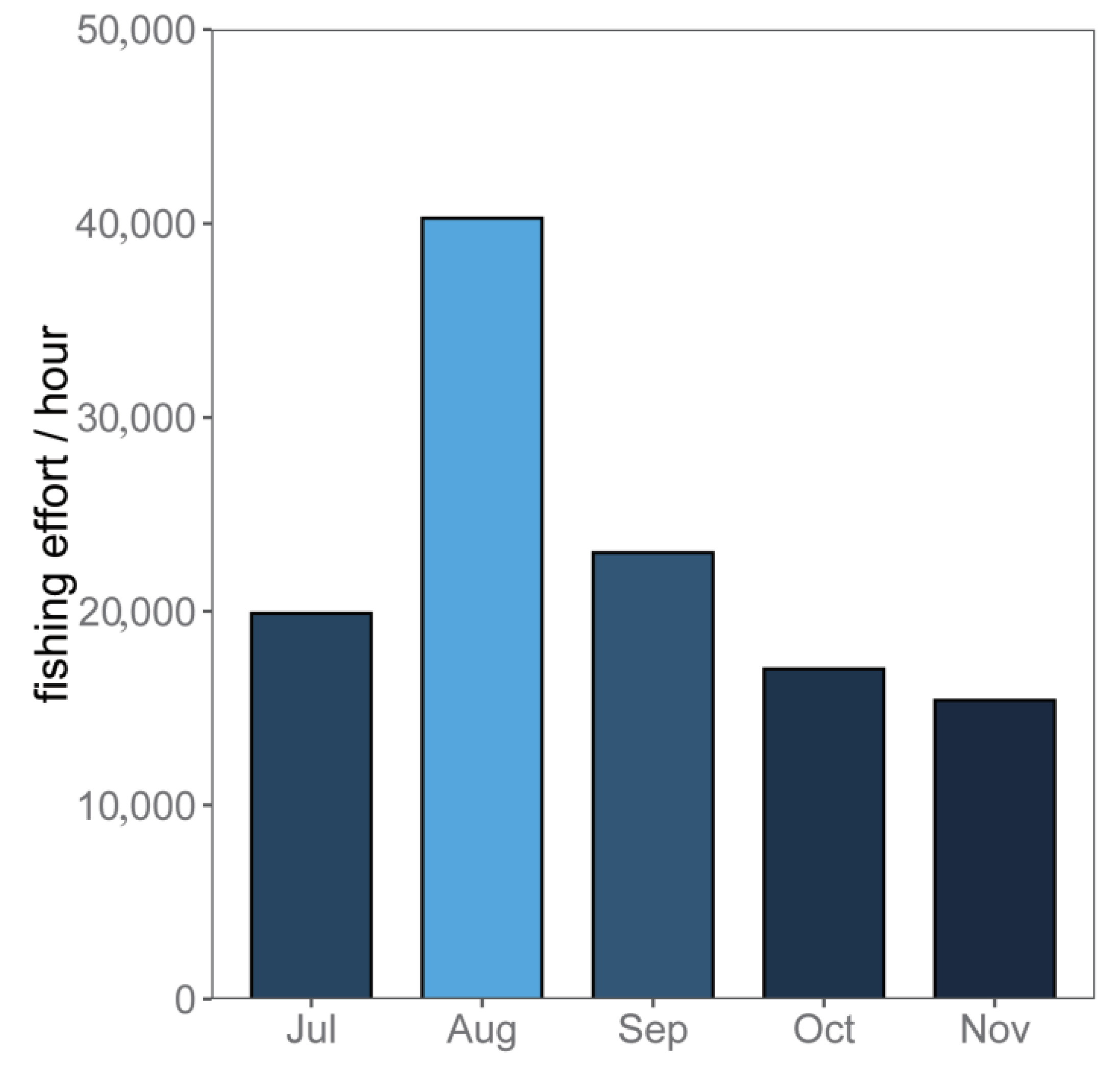
3.1. Monthly Distribution of Fishing Effort

Figure 3 showed the distribution of months for the average monthly fishing effort from July to November in 2017 to 2020. The fishing effort of the squid-jigging vessels increased gradually from July to August. After August, the fishing effort started to decrease. In August, the fishing effort reached a maximum at approximately 40,275 h. In November, the fishing effort was at its minimum at approximately 15,407 h. Furthermore, the fishing effort was higher during July to September than during October to November.

3.2. Variations in the Gravity of Fishing Effort

Obvious variations in the center of gravity of the squid-jigging vessel fishing effort occurred from July to November in 2017–2020 (Figure 4). In July, the center of gravity of the fishing effort was in the vicinity of ${174.2}^{\circ }\mathrm{E}$, ${43.1}^{\circ }\mathrm{N}$, and then the center of gravity of the fishing effort shifted to the northwest. In August, the center of gravity of the fishing effort was at the northernmost end, positioned in the vicinity of ${166}^{\circ }\mathrm{E}$, ${43.7}^{\circ }\mathrm{N}$, and then it shifted to the southwest. In September, the center of gravity of the fishing effort was in the vicinity of ${161.8}^{\circ }\mathrm{E}$, ${43.3}^{\circ }\mathrm{N}$, and it continued to move in a south-westerly direction. In October, the center of gravity of the fishing effort was in the vicinity of ${156.5}^{\circ }\mathrm{E}$, ${42.1}^{\circ }\mathrm{N}$. In November, the center of gravity of the fishing effort was at the southernmost end, positioned in the vicinity of ${152.1}^{\circ }\mathrm{E}$, ${41.7}^{\circ }\mathrm{N}$.

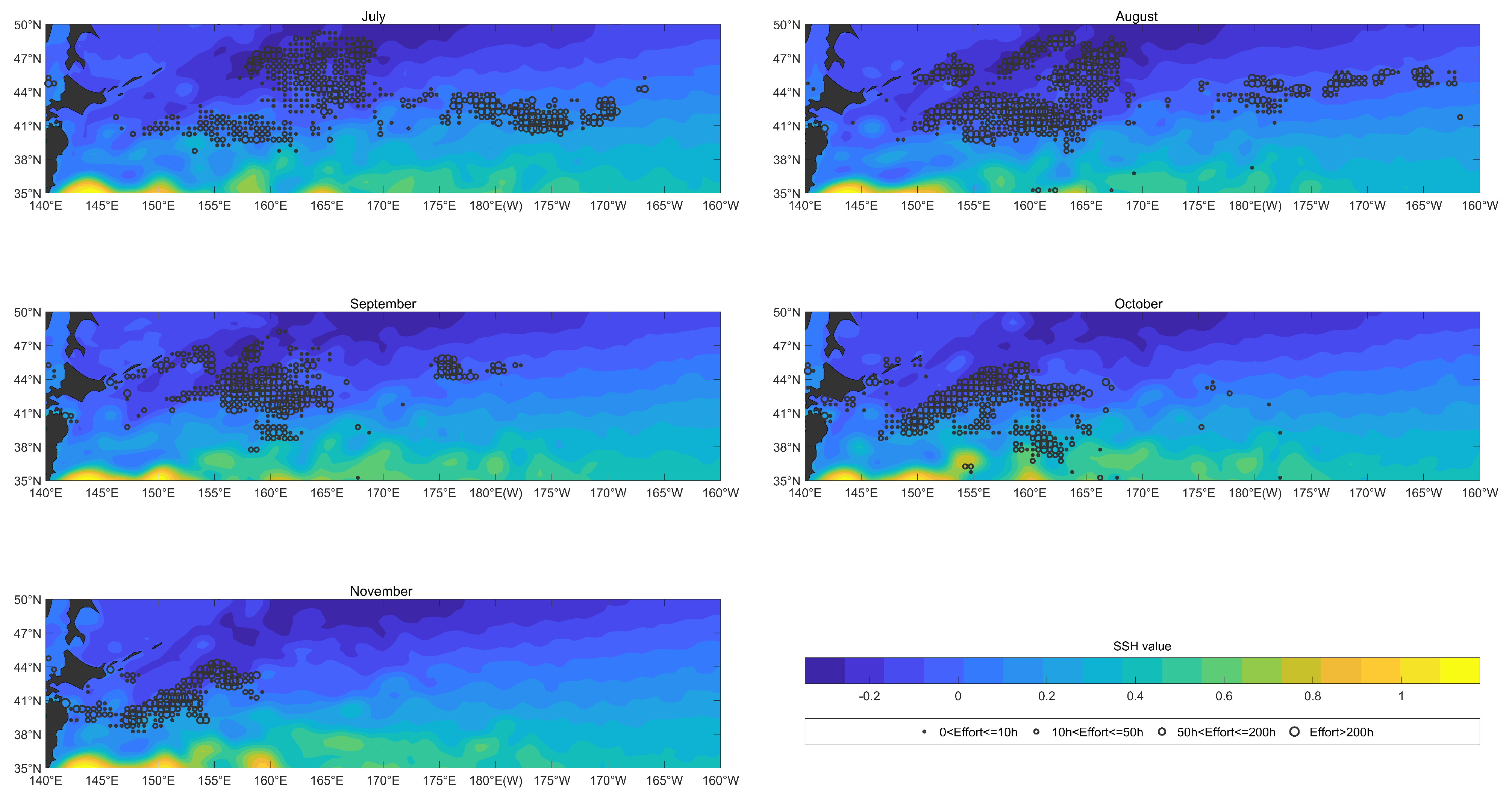
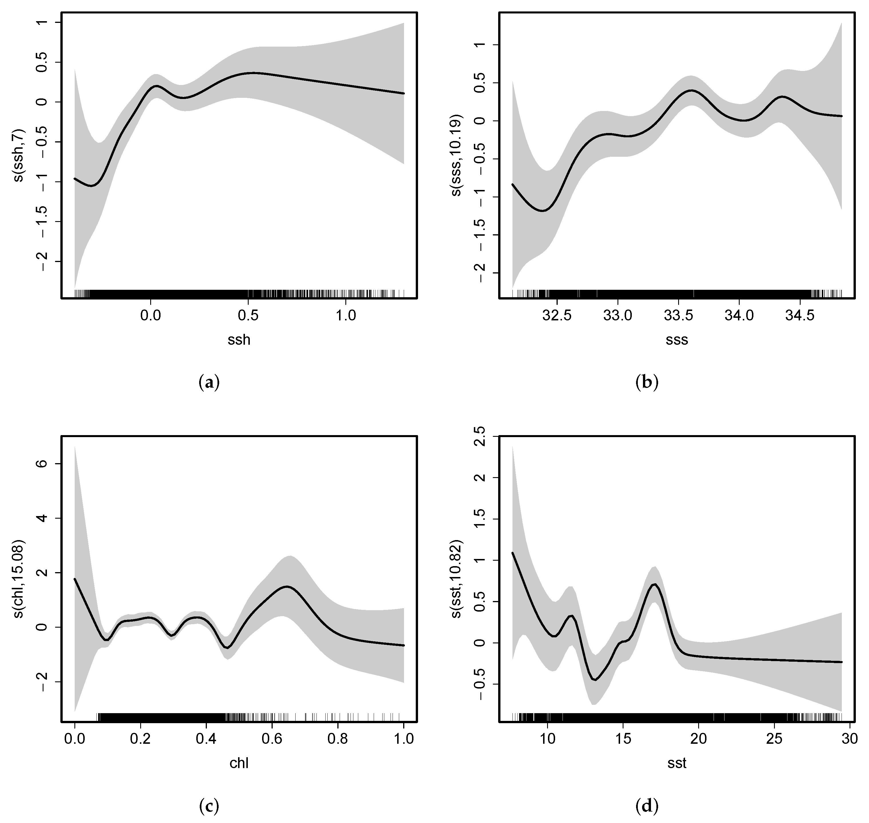
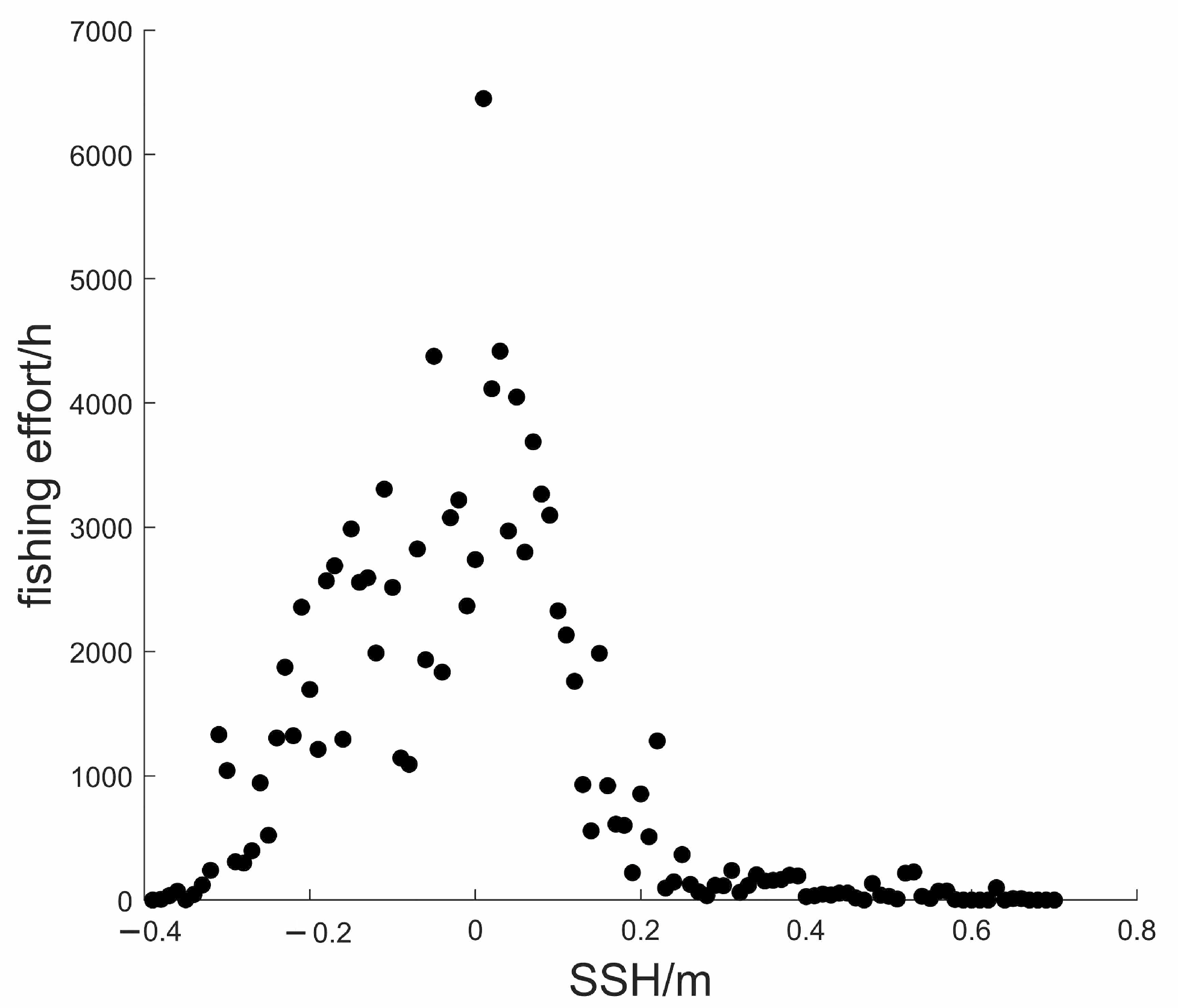
3.3. The Relationship between Fishing Effort and SSH

As shown in Figure 5, the variation in SSH was not obvious from July to November in 2017–2020. The areas with SSH values were concentrated along the coast of the Japanese Archipelago to the east into the sea in the vicinity of ${140}^{\circ }\mathrm{E}\sim {160}^{\circ }\mathrm{E}$, ${35}^{\circ }\mathrm{N}$, with SSH values above 1 m in this area, and there was almost no fishing effort distributed within this area.

From July to November, the fishing effort distribution areas were mainly in areas with low SSHs. In July, the fishing effort was mainly distributed in the areas with $-0.25\mathrm{m}\sim 0.16\mathrm{m}$ of SSH, and there was considerable fishing effort in the eastern area which was in the vicinity of ${175}^{\circ }\mathrm{E}\sim {170}^{\circ }\mathrm{W}$, ${40}^{\circ }\mathrm{N}\sim {44}^{\circ }\mathrm{N}$ with $0\sim 0.2\mathrm{m}$ of SSH. In August, the fishing effort was mainly distributed in the areas with $-0.27\mathrm{m}\sim 0.17\mathrm{m}$ of SSH. Compared with July, there was a little fishing effort in the eastern area in August. In September, the fishing effort was mainly distributed in the areas with $-0.23\mathrm{m}\sim 0.1\mathrm{m}$ of SSH. From October to November, the fishing effort was mainly distributed in the areas with $-0.2\mathrm{m}\sim 0.2\mathrm{m}$ of SSH.

Figure 6 shows that the fishing effort was distributed in areas with an SSH range of $-0.27\mathrm{m}\sim 0.2\mathrm{m}$. The average SSH was 0.16 m. The fishing effort was maximum when SSH was 0 m.

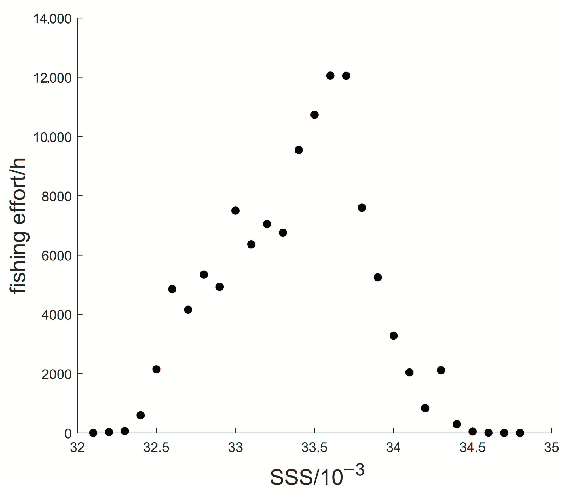
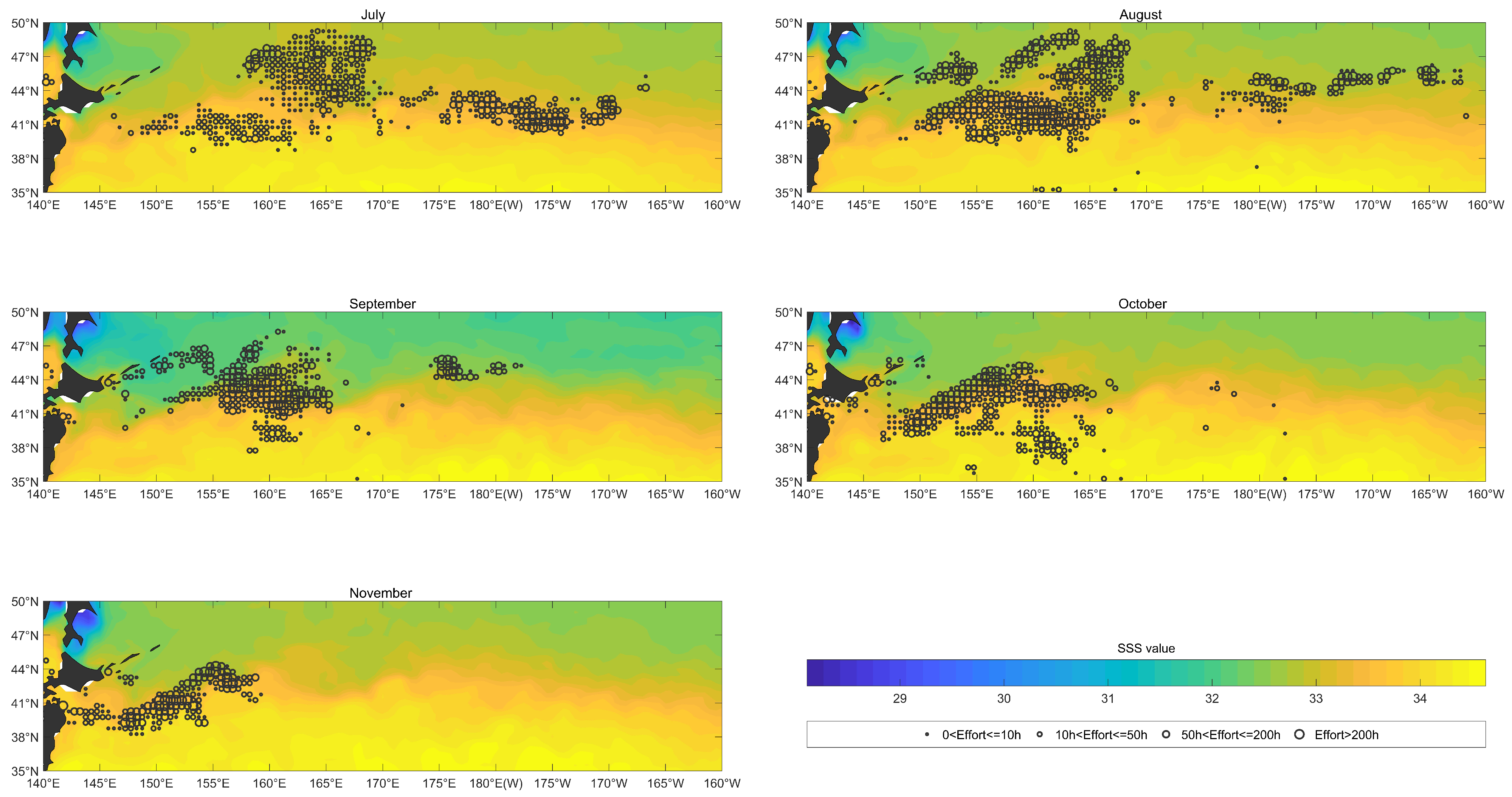
3.4. The Relationship between Fishing Effort and SSS

Figure 7 showed that the considerable fishing effort was mainly distributed in the areas with $32\times {10}^{-3}\sim 34\times {10}^{-3}$ from July to November. There was almost no fishing effort in the area in which SSS was greater than $34\times {10}^{-3}$.

Figure 8 showed that the fishing effort was distributed in areas with an SSS range of $32.5\times {10}^{-3}\sim 34.1\times {10}^{-3}$. The average SSS was $33.5\times {10}^{-3}$. The fishing effort was maximum when SSS was $33.5\times {10}^{-3}$.

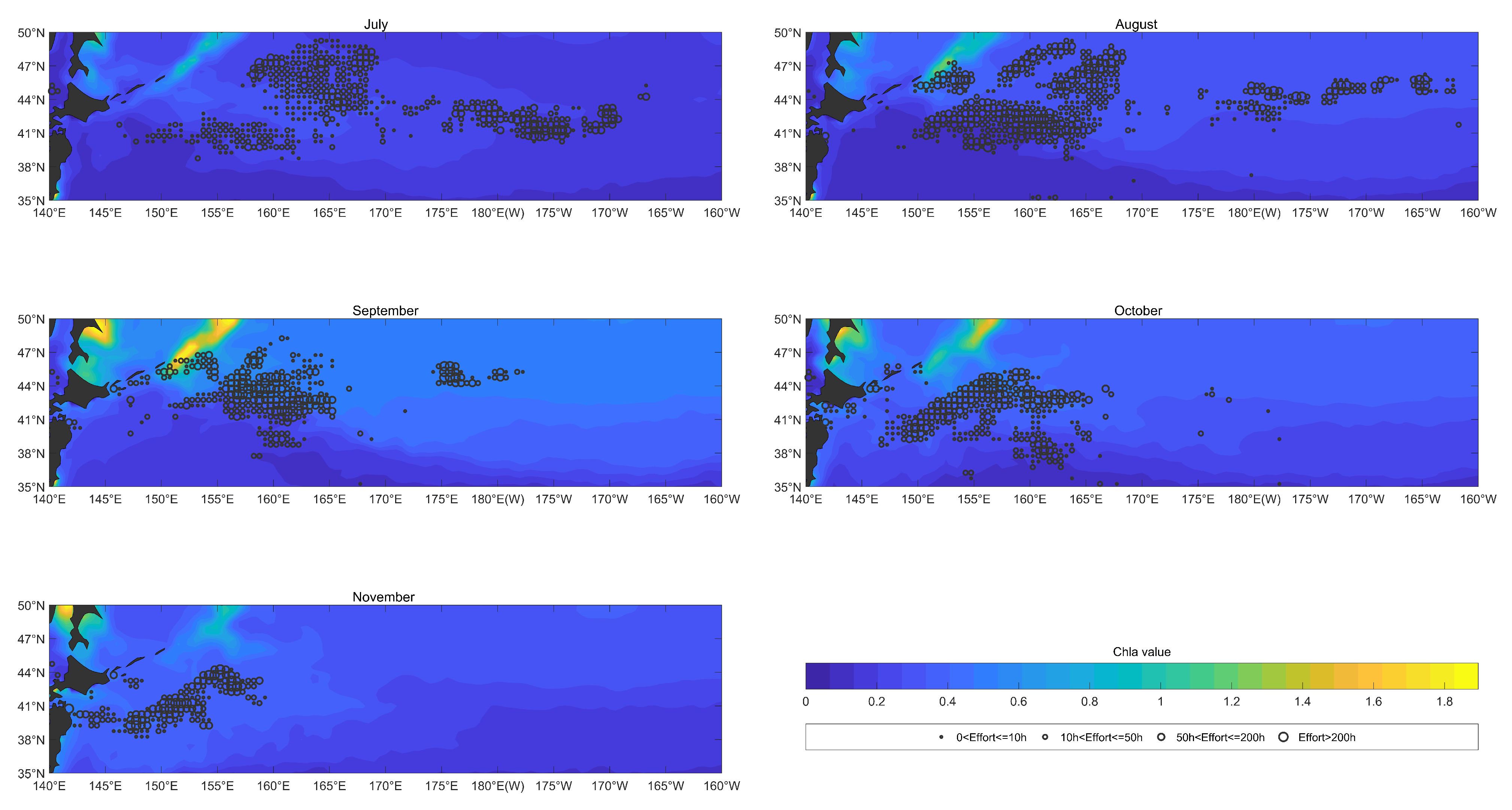
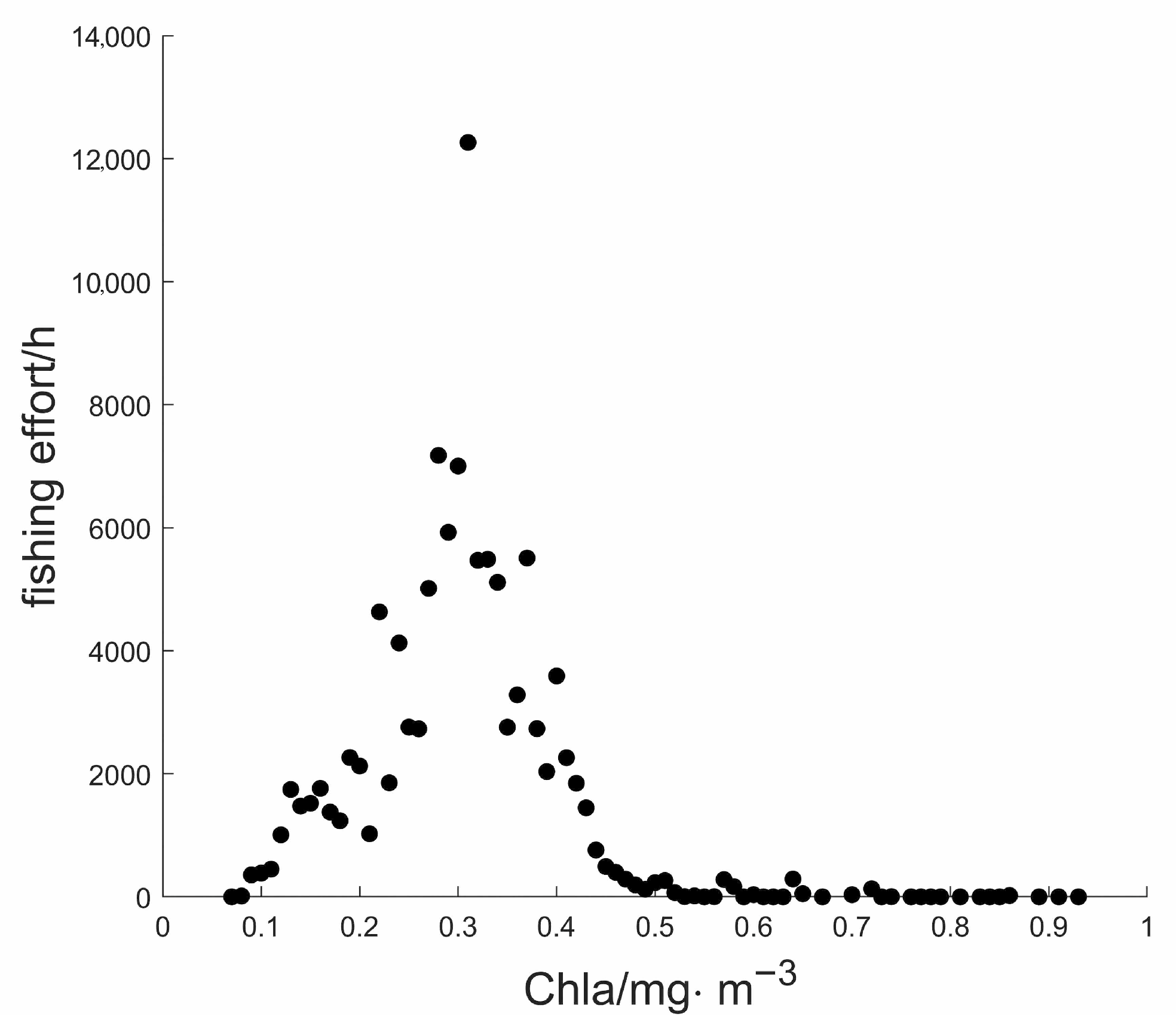
3.5. The Relationship between Fishing Effort and Chla

As shown in Figure 9, the Chla was mainly distributed spatially in a latitudinal direction from July to November between 2017 and 2020, with high Chla in the north and low Chla in the south. The fishing effort was mainly distributed in the area with Chla over $0.2\mathrm{mg}·{\mathrm{m}}^{-3}$ from July to November. In July, Chla was higher in the northern area at ${140}^{\circ }\mathrm{E}\sim {170}^{\circ }\mathrm{W}$, ${39}^{\circ }\mathrm{N}\sim {50}^{\circ }\mathrm{N}$, and the fishing effort was also mainly distributed in this region. In August and September, Chla began to contract to the north, with the latitudinal range decreasing to approximately ${41}^{\circ }\mathrm{N}\sim {50}^{\circ }\mathrm{N}$. In October, Chla began to spread southward again. In November, high Chla values were the most widely distributed, covering almost the entire study area. The distribution of the fishing effort moved southward with Chla from October to November.

Almost no fishing effort occurred in the areas with Chla concentrations below $0.1\mathrm{mg}·{\mathrm{m}}^{-3}$. In July, the fishing effort was mainly distributed in areas where the range of Chla concentrations was $0.25\mathrm{mg}·{\mathrm{m}}^{-3}\sim 0.3\mathrm{mg}·{\mathrm{m}}^{-3}$. In August and September, the fishing effort was mainly distributed in areas where the range of Chla concentrations was $0.1\mathrm{mg}·{\mathrm{m}}^{-3}\sim 0.3\mathrm{mg}·{\mathrm{m}}^{-3}$. In October, the fishing effort was mainly distributed in areas where the range of Chla concentrations was $0.2\mathrm{mg}·{\mathrm{m}}^{-3}\sim 0.3\mathrm{mg}·{\mathrm{m}}^{-3}$. In November, the fishing effort was mainly distributed in areas where the range of Chla concentrations was $0.3\mathrm{mg}·{\mathrm{m}}^{-3}\sim 0.4\mathrm{mg}·{\mathrm{m}}^{-3}$.

Figure 10 showed that the fishing effort was distributed in areas with the range of Chla at $0.21\mathrm{mg}·{\mathrm{m}}^{-3}\sim 0.43\mathrm{mg}·{\mathrm{m}}^{-3}$. The average Chla was $0.46\mathrm{mg}·{\mathrm{m}}^{-3}$. The fishing effort was at its maximum when Chla was $0.31\mathrm{mg}·{\mathrm{m}}^{-3}$.

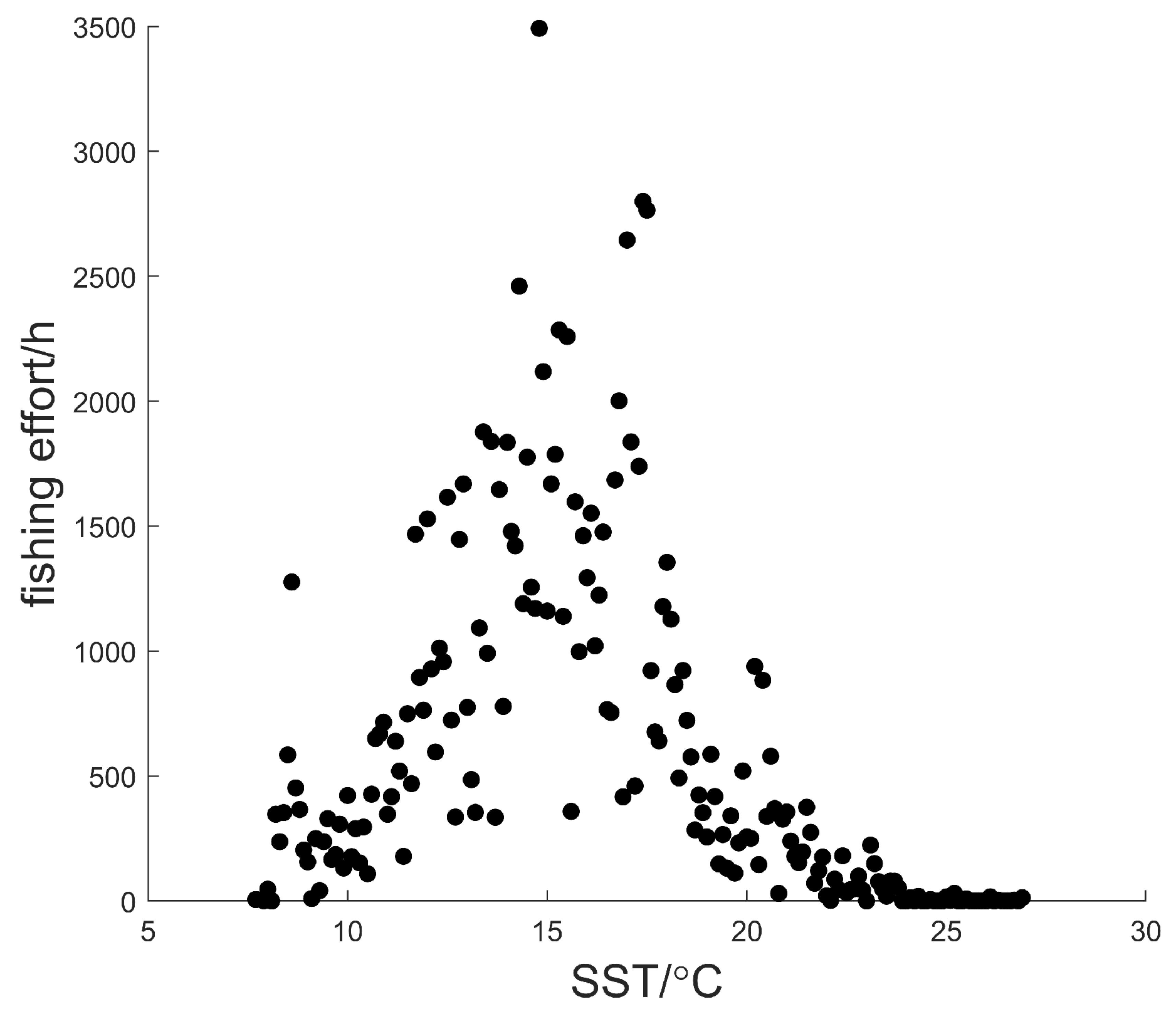
3.6. The Relationship between Fishing Effort and SST

As shown in Figure 11, SST was mainly distributed spatially in a latitudinal direction from July to November from 2017 to 2020, with high SST in the south and low SST in the north. From a temporal point of view, summer in the Northern Hemisphere is in July and August, the SST in the southern area is higher, and the area covered by high-temperature water is large. Autumn to early winter occurs from September to November. High-temperature water began to fade from north to south, and the area of low-temperature waters began to increase southward. Hence, there were obvious seasonal differences in SST variation.

Almost no fishing effort was distributed in waters with SST over $21{}^{\circ }\mathrm{C}$ from July to November. In July, the fishing effort was concentrated in waters with sea surface temperatures between $8{}^{\circ }\mathrm{C}$ and $20{}^{\circ }\mathrm{C}$. In August, the area of high SST waters in the North Pacific expanded from south to north, and the fishing effort area moved northward with the low SST waters, and the SST of the fishing effort area was between $10{}^{\circ }\mathrm{C}$ and $21{}^{\circ }\mathrm{C}$. The area of waters with a high SST in the North Pacific decreased from north to south from September to November, and the area of low-temperature waters began to increase southward, with the fishing effort area moving southward with low-temperature waters. During this period, the SST of the fishing effort area was between $10{}^{\circ }\mathrm{C}$ and $21{}^{\circ }\mathrm{C}$ in September and October, and the SST of the fishing effort area was between $8{}^{\circ }\mathrm{C}$ and $19{}^{\circ }\mathrm{C}$ in November.

Figure 12 shows that the fishing effort was distributed in areas with an SST range of $10.9{}^{\circ }\mathrm{C}\sim 20.6{}^{\circ }\mathrm{C}$. The average SST was $17.4{}^{\circ }\mathrm{C}$. The fishing effort was at its maximum when SST was $14.8{}^{\circ }\mathrm{C}$.

3.7. Generalized Additive Model

3.7.1. Analysis of GAM Results

The F-test showed that the model of the final GAM obtained in a stepwise manner using the AIC retained latitude, longitude, SSH, SSS, Chla and SST at the significance level $\alpha =0.05$ (

Table 1. Statistical parameters of GAM model.

Formula	AIC	Deviance Explained (%)	${\mathit{R}}_{\mathit{adj}}^2$	Deviance
$ln(effort+0.1)\sim \mathrm{s}(Lon,Lat)$	27,049.15	37.5	0.360	25,835.54
$ln(effort+0.1)\sim \mathrm{s}(Lon,Lat)+\mathrm{s}\left(SST\right)$	26,920.17	38.6	0.371	25,357.38
$ln(effort+0.1)\sim \mathrm{s}(Lon,Lat)+\mathrm{s}\left(SST\right)+\mathrm{s}\left(SSH\right)$	26,866.01	39.4	0.377	25,048.13
$ln(effort+0.1)\sim \mathrm{s}(Lon,Lat)+\mathrm{s}\left(SST\right)+\mathrm{s}\left(SSH\right)+\mathrm{s}\left(SSS\right)$	26,840.66	39.7	0.380	24,897.19
$ln(effort+0.1)\sim \mathrm{s}(Lon,Lat)+\mathrm{s}\left(SST\right)+\mathrm{s}\left(SSH\right)+\mathrm{s}\left(SSS\right)+\mathrm{s}\left(Chla\right)$	26,758.20	40.8	0.389	24,458.48

and

Table 2. F-test for significance of non-parametric effects.

Variable	Degrees of Freedom	F-Value	p-Value
Lat, Lon	147.515	15.823	<$2\times {10}^{-16}$
SST	10.819	7.407	<$2\times {10}^{-16}$
SSH	7.001	3.362	0.000527
SSS	10.186	3.514	$1.78\times {10}^{-5}$
Chla	15.084	5.641	<$2\times {10}^{-16}$

). The final GAM model at the significance level of $\alpha =0.05$ showed that the variation in fishing effort explained by all variables was 40.8%, and the coefficient of determination was 0.389 (Table 1). Of the variables, the synergistic impacts of longitude and latitude contributed the most to the variation in fishing effort (Table 1), and its corresponding F-value is also the largest (Table 2). In the four marine environmental variables, according to their contribution to the model, we had SST > Chla > SSH > SSS. The sequence of their corresponding F-value was in the same order as above.

3.7.2. Impact of Latitude and Longitude on Fishing Effort

The solid black line in Figure 13a indicated the area where the fishing effort of squid-jigging vessels in the North Pacific Ocean was mainly distributed. The red dashed line (a positive standard deviation) and the green dashed line (a negative standard deviation) indicate confidence intervals for the area of operation of squid-jigging vessels. The area showed a closed curve of one layer, distributed in the regions of ${144}^{\circ }\mathrm{E}\sim {170}^{\circ }\mathrm{E}$, ${38}^{\circ }\mathrm{N}\sim {50}^{\circ }\mathrm{N}$ and ${172}^{\circ }\mathrm{E}\sim {160}^{\circ }\mathrm{W}$, ${40}^{\circ }\mathrm{N}\sim {46}^{\circ }\mathrm{N}$. A three-dimensional spatial plot of the impact of latitude and longitude on the fishing effort (Figure 13b) showed that two mountain range bumps appeared in the fishing area, corresponding to the areas of ${144}^{\circ }\mathrm{E}\sim {170}^{\circ }\mathrm{E}$, ${38}^{\circ }\mathrm{N}\sim {50}^{\circ }\mathrm{N}$ and ${172}^{\circ }\mathrm{E}\sim {160}^{\circ }\mathrm{W}$, ${40}^{\circ }\mathrm{N}\sim {46}^{\circ }\mathrm{N}$ in Figure 13a. The favorable area for fishing effort was in ${152}^{\circ }\mathrm{E}\sim {165}^{\circ }\mathrm{E}$, ${41}^{\circ }\mathrm{N}\sim {44}^{\circ }\mathrm{N}$ by combining Figure 4 and Figure 13a.

3.7.3. Impacts of Different Marine Environmental Factors on Fishing Effort

Figure 14a showed that the impact of SSH on fishing effort was positively correlated when SSH was between −0.2 m and 0 m. The impact of SSH on fishing effort was relatively stable when SSH was between 0 m and 0.5 m. The suitable range of SSH for fishing effort was −0.2 m ∼ 0.2 m, and a range of SST that was more beneficial to fishing squid was between 0 ∼ 0.2 m. Figure 14b showed that the impact of SSS on fishing effort was positively correlated when SSS was between $32.5\times {10}^{-3}$ and $33.5\times {10}^{-3}$. The impact of SSS on fishing effort gradually decreased as SSS over $34.5\times {10}^{-3}$ or below $32.5\times {10}^{-3}$. The favorable range of SSS for fishing effort was $33\times {10}^{-3}\sim 34\times {10}^{-3}$. Figure 14c showed that the impact of Chla on fishing effort was relatively stable when Chla was between $0.1\mathrm{mg}·{\mathrm{m}}^{-3}$ and $0.4\mathrm{mg}·{\mathrm{m}}^{-3}$. The impact of Chla on fishing effort decreased as Chla over $0.4\mathrm{mg}·{\mathrm{m}}^{-3}$. The favorable range of Chla for fishing effort was $0.2\mathrm{mg}·{\mathrm{m}}^{-3}\sim 0.4\mathrm{mg}·{\mathrm{m}}^{-3}$. Figure 14d showed that the impact of SST on fishing effort was negatively correlated when SST was between $11{}^{\circ }\mathrm{C}$ and $13{}^{\circ }\mathrm{C}$. Nevertheless, when SST was between $13{}^{\circ }\mathrm{C}$ and $17{}^{\circ }\mathrm{C}$, the impact of SST on fishing effort gradually increased, with the strongest impact at approximately $17{}^{\circ }\mathrm{C}$. The suitable range of SST for fishing effort was $14{}^{\circ }\mathrm{C}\sim 20{}^{\circ }\mathrm{C}$, and a preferred SST was in the range of $15{}^{\circ }\mathrm{C}\sim 18{}^{\circ }\mathrm{C}$.

3.7.4. The GAM at Different Spatial Resolutions

At resolutions of ${0.1}^{\circ }\times 0.1^{\circ }$, ${0.25}^{\circ }\times {0.25}^{\circ }$ and $1^{\circ }\times 1^{\circ }$, three final GAM models at the significance level of $\alpha =0.05$ showed that deviance explained by the models was 20.5%, 30.4% and 50.5%, respectively (

Table 3. Statistical parameters of GAM model (${0.1}^{\circ }\times {0.1}^{\circ }$).

Formula	AIC	Deviance Explained (%)	${\mathit{R}}_{\mathit{adj}}^2$	Deviance
$ln(effort+0.1)\sim \mathrm{s}(Lon,Lat)$	299,371.3	17.2	0.170	160,078.5
$ln(effort+0.1)\sim \mathrm{s}(Lon,Lat)+\mathrm{s}\left(SST\right)$	297,990.5	18.4	0.182	157,696.8
$ln(effort+0.1)\sim \mathrm{s}(Lon,Lat)+\mathrm{s}\left(SST\right)+\mathrm{s}\left(SSH\right)$	297,534.8	18.6	0.186	156,812.3
$ln(effort+0.1)\sim \mathrm{s}(Lon,Lat)+\mathrm{s}\left(SST\right)+\mathrm{s}\left(SSH\right)+\mathrm{s}\left(SSS\right)$	296,792.2	19.6	0.193	155,368.4
$ln(effort+0.1)\sim \mathrm{s}(Lon,Lat)+\mathrm{s}\left(SST\right)+\mathrm{s}\left(SSH\right)+\mathrm{s}\left(SSS\right)+\mathrm{s}\left(Chla\right)$	295,658.5	20.5	0.202	153,577.5

,

Table 4. Statistical parameters of GAM model (${0.25}^{\circ }\times {0.25}^{\circ }$).

Formula	AIC	Deviance Explained (%)	${\mathit{R}}_{\mathit{adj}}^2$	Deviance
$ln(effort+0.1)\sim \mathrm{s}(Lon,Lat)$	79,349.8	26.8	0.262	61,522.3
$ln(effort+0.1)\sim \mathrm{s}(Lon,Lat)+\mathrm{s}\left(SST\right)$	78,989.7	28.1	0.274	60,388.2
$ln(effort+0.1)\sim \mathrm{s}(Lon,Lat)+\mathrm{s}\left(SST\right)+\mathrm{s}\left(SSH\right)$	78,842.8	28.7	0.280	59,888.4
$ln(effort+0.1)\sim \mathrm{s}(Lon,Lat)+\mathrm{s}\left(SST\right)+\mathrm{s}\left(SSH\right)+\mathrm{s}\left(SSS\right)$	78,698.6	29.4	0.286	59,307.5
$ln(effort+0.1)\sim \mathrm{s}(Lon,Lat)+\mathrm{s}\left(SST\right)+\mathrm{s}\left(SSH\right)+\mathrm{s}\left(SSS\right)+\mathrm{s}\left(Chla\right)$	78,430.6	30.4	0.295	58,470.8

and

Table 5. Statistical parameters of GAM model ($1^{\circ }\times 1^{\circ }$).

Formula	AIC	Deviance Explained (%)	${\mathit{R}}_{\mathit{adj}}^2$	Deviance
$ln(effort+0.1)\sim \mathrm{s}(Lon,Lat)$	8977.0	46.3	0.435	10,229.0
$ln(effort+0.1)\sim \mathrm{s}(Lon,Lat)+\mathrm{s}\left(SST\right)$	8937.9	47.9	0.449	9919.5
$ln(effort+0.1)\sim \mathrm{s}(Lon,Lat)+\mathrm{s}\left(SST\right)+\mathrm{s}\left(SSH\right)$	8933.2	48.2	0.451	9864.8
$ln(effort+0.1)\sim \mathrm{s}(Lon,Lat)+\mathrm{s}\left(SST\right)+\mathrm{s}\left(SSH\right)+\mathrm{s}\left(SSS\right)$	8903.6	49.4	0.461	9632.4
$ln(effort+0.1)\sim \mathrm{s}(Lon,Lat)+\mathrm{s}\left(SST\right)+\mathrm{s}\left(SSH\right)+\mathrm{s}\left(SSS\right)+\mathrm{s}\left(Chla\right)$	8893.6	50.5	46.8	9439.5

). The deviance explained by the model was increased as spatial resolution increased. The synergistic effect of latitude and longitude on fishing effort was still the greatest no matter how the spatial resolution changed. For the four marine environmental variables, no matter how the spatial resolution changed, the SST always had the largest contribution to the model. The order of contribution of the other three marine environmental variables were changed with the change in spatial resolution (Table 3, Table 4 and Table 5). Moreover, the spatial distribution of fishing effort was essentially the same when the spatial resolutions were not the same (Figure 13a and see Figures S1a, S3a and S5a in the Supplementary Materials). When the spatial resolution was $1^{\circ }\times 1^{\circ }$, the trend in the influence of the marine environment on fishing effort was different from the remaining three, especially for SSH. The influence of the marine environment on fishing effort fluctuates greatly and the trend was not obvious (see Figures S2a–d, S4a–d and S6a–d in the Supplementary Materials).

3.7.5. The Results of GAM without Latitude and Longitude

The final GAM model without latitude and longitude showed that the deviance explained by the model was 16.3% at the significance level of $\alpha =0.05$ (

Table 6. Statistical parameters of GAM model (${0.5}^{\circ }\times {0.5}^{\circ }$, not latitude and longitude).

Formula	AIC	Deviance Explained (%)	${\mathit{R}}_{\mathit{adj}}^2$	Deviance
$ln(effort+0.1)\sim \mathrm{s}\left(SST\right)$	28,943.6	11.4	0.112	36,620.3
$ln(effort+0.1)\sim \mathrm{s}\left(SST\right)+\mathrm{s}\left(SSH\right)$	28,841.4	13.1	0.128	35,920.6
$ln(effort+0.1)\sim \mathrm{s}\left(SST\right)+\mathrm{s}\left(SSH\right)+\mathrm{s}\left(SSS\right)$	28,677.3	15.8	0.153	34,794.8
$ln(effort+0.1)\sim \mathrm{s}\left(SST\right)+\mathrm{s}\left(SSH\right)+\mathrm{s}\left(SSS\right)+\mathrm{s}\left(Chla\right)$	28,652.6	16.3	0.156	34,593.0

). The SST had the greatest influence on fishing effort, followed by SSS. The contribution of Chla was lowest in the GAM model. In addition, intervals of the suitable marine environmental variables for fishing effort obtained from this GAM model were generally consistent with Figure 14a–d (see Figure S7 in the Supplementary Materials).

4. Discussion

4.1. Spatial and Temporal Distribution of Fishing Effort

There was obvious seasonal variability in the impact of the month factor on fishing effort in this study (Figure 3). The fishing effort from October to November was lower than from July to September. The results were similar to those in the study of Yu et al. [6]. The maximum and minimum value of fishing effort occurred in August and November, respectively, in this study. The squid population migrated to the Oyashio Current Frontal Zone and the surrounding waters between ${40}^{\circ }\mathrm{N}$ and ${46}^{\circ }\mathrm{N}$ from August to October during the main fishing seasons [6]. Fan et al. [42] suggested that O. bartramii migrate northward to feed in July and August. Tian et al. [43] and Wei et al. [44] suggested that sexually mature male O. bartramii individuals start migrating south to spawn in October to November, while female O. bartramii individuals are sexually mature later and generally migrate south to spawn in November to December. Therefore, the squid breeding was mainly in the traditional fishing grounds of China. Accordingly, the fishing effort was increased due to large number of vessels in August. Nevertheless, the squid migrated south to spawn in November, and the fishing effort was low. Furthermore, the above discussion revealed the reason for the spatial variation in fishing effort from July to November in Figure 4.

According to the results of GAM, there was a significant impact for latitude and longitude on fishing effort (Table 1). The area where fishing vessels were concentrated was faulted near longitude ${170}^{\circ }\mathrm{E}$ (Figure 13a). This phenomenon was mainly caused by squid migration in July to August. The range of longitude beneficial for fishing tended to be between ${152}^{\circ }\mathrm{E}$ and ${165}^{\circ }\mathrm{E}$ (Figure 3, Figure 4 and Figure 13a). As shown in Figure 4 and Figure 13a, the range of latitude beneficial for fishing was between ${41}^{\circ }\mathrm{N}$ and ${44}^{\circ }\mathrm{N}$. This sea area is formed by the confluence of the warm Kuroshio and cold Oyashio Currents [45]. High horizontal temperature gradient, high nutrient upwelling, meandering eddies, and front zones provide favorable environmental conditions to yield a highly productive abundance for O. bartramii [46]. Thus, the fishing effort was high in the sea area. Furthermore, Yu et al. [41] suggested that the favorable area for squid was in ${40}^{\circ }\mathrm{N}\sim {43.5}^{\circ }\mathrm{N}$, ${153}^{\circ }\mathrm{E}\sim {161}^{\circ }\mathrm{E}$. The range of latitude is consistent with the results in this paper, but the range of longitude is less than that in this paper. The reason might be that the east of the study area was wide.

4.2. Impacts of Marine Conditions on Fishing Effort

Variations in the marine environment lead to variations in the distribution of fish stocks, thus indirectly affecting the spatial distribution of fishing vessel operations. Previous studies suggested that O. bartramii, as an opportunistic species, is extremely susceptible to climatic and environmental variability at a range of spatial and temporal scales [47].

Chen et al. [48] suggested that a suitable water temperature was beneficial to O. bartramii in terms of gathering at fishing grounds. In this study, the fishing effort might be related to the increased temperature of water due to the high fishing effort in summer (Figure 3). Yu et al. [49] suggested that the optimum range of SST is $14{}^{\circ }\mathrm{C}\sim 18{}^{\circ }\mathrm{C}$ for O. bartramii in fishing season in the North Pacific Ocean. Furthermore, Wang et al. [50] reported that the suitable range of SST was >$15.5{}^{\circ }\mathrm{C}$ and increasing water temperatures were beneficial to O. bartramii at the surface. These conclusions were basically similar to the results of this paper. The optimum range of SST derived from Japanese fishing grounds was $15{}^{\circ }\mathrm{C}\sim 17{}^{\circ }\mathrm{C}$ [5]. The difference is due to the spatial sample bias and data limitations.

SSH is influenced by variations in the dynamics of ocean topography, which can transport nutrients and salt from deep seawater to the surface to create an environment conducive to fish habitats. The fishing effort was decreased when SSH was too high (Figure 5 and Figure 14a). Fan et al. [51] suggested that at $\mathrm{SSH}>0$, the yields of O. bartramii are greater in the North Pacific Ocean, especially at SSH in $0\sim 0.3\mathrm{m}$; at $\mathrm{SSH}<0$, yields for O. bartramii are increasingly lower. The phenomenon might be due to the migration of squid southward in October and November before the fishing vessels arrived. Therefore, the fishing effort was decreased in the area where SSH was too high.

Irene et al. [52] concluded that Chla is related to the availability of food and is another useful factor in predicting the distribution of squid habitat. As shown in Figure 9, the fishing effort of squid-jigging vessels was mainly distributed in the area where Chla was between $0.1\mathrm{mg}·{\mathrm{m}}^3$ and $0.4\mathrm{mg}·{\mathrm{m}}^3$ from July to November. The phenomenon of fishing effort increasing with increasing Chla was not found. The results of GAM showed that the impact of Chla on fishing effort was not obvious in the favorable range of Chla for fishing effort. The reason might be migration of squid to the north into low temperature waters from July to August, and Chla was high in the area of lower water temperature. The water temperature decreased in the South Sea area from September to November. Meanwhile, squid began to migrate to the south. Yu et al. [49] suggested that the optimum range of Chla is between $0.2\mathrm{mg}·{\mathrm{m}}^3$ and $0.5\mathrm{mg}·{\mathrm{m}}^3$ for O. bartramii. This conclusion is basically similar to the results in this paper. Wang et al. [53] suggested that Chlorophyll-a gradients have a significant influence on squid fishing grounds not only in the offshore region, but also in the open sea region. Thus, the Chlorophyll-a gradients could be a focus for future research.

Alabia et al. [5] suggested that the potential squid fishing ground was largely explained by SSS. Alabia et al. [5] also suggested that the favorable SSS for fishing squid were $33.8\times {10}^{-3}\sim 34.8\times {10}^{-3}$ and $33.7\times {10}^{-3}\sim 34.3\times {10}^{-3}$ in the winter and summer, respectively. The conclusion was similar to the results of this study. However, the results from GAM model suggested that SSS showed the least influence on fishing location.

4.3. The GAM Models of a Control Group

The deviance explained by GAM which was constructed by using data with a spatial resolution of ${0.1}^{\circ }\times {0.1}^{\circ }$ or ${0.25}^{\circ }\times {0.25}^{\circ }$ was low (Table 3 and Table 4). The reason might be that there were some details that had not been taken into account. Furthermore, the details of the fitted curve fluctuate significantly when the spatial resolution was ${0.1}^{\circ }\times {0.1}^{\circ }$ or ${0.25}^{\circ }\times {0.25}^{\circ }$. This suggested that there was no obvious trend in the impacts of the marine environment on fishing effort. By using data with a spatial resolution of $1^{\circ }\times 1^{\circ }$, the deviance explained by GAM was 50.5% (Table 5), which was higher than the model with a spatial resolution of ${0.5}^{\circ }\times {0.5}^{\circ }$. Nevertheless, although there was a high value of the deviance explained by the model when the spatial resolution was $1^{\circ }\times 1^{\circ }$, the obviously high spatial resolution smoothed out a lot of details, which meant it was unable to reflect the real situation. The GAM bias using data with a spatial resolution of ${0.5}^{\circ }\times {0.5}^{\circ }$, and without latitude and longitude, explained very little of the deviance. This phenomenon indicated that the migration of O. bartramii from north to south had a significant influence on the spatial distribution of squid-jigging vessels. Therefore, the fishing effort was not entirely determined by the marine environment.

5. Conclusions

In this study, the fishing effort calculated from AIS was adopted to detect the monthly spatial and temporal distribution patterns for North Pacific squid-jigging fishing vessels and their relationship with the marine environment. The GAM model was established by four key variables including SST, SSH, SSS and Chla. The spatial and temporal distribution of squid-jigging fishing operations showed significant monthly variation and was influenced by the marine environment. The results obtained in this paper from the analysis using AIS data and that using fish catch data are generally consistent, showing that the AIS data of squid-jigging fishing vessels can be used to analyse variations in squid in the Northwestern Pacific Ocean. In the future, flexible temporal and spatial data should be provided to address the issues. The tracking data of the squid-jigging vessels in this paper were obtained from a large number of countries and regions, with a more comprehensive sample representation and spatial distribution of data. Thus, this paper can better spatially represent the fishing pressure on these North Pacific fisheries resources.

References

1. Yu, W.; Wen, J.; Zhang, Z.; Chen, X.; Zhang, Y. Spatio-temporal variations in the potential habitat of a pelagic commercial squid. J. Mar. Syst. 2020, 206, 103339. [Google Scholar] [CrossRef]
2. Wang, Y.; Chen, X.; Fang, Z. Effects of marine environment variation on the growth of neno flying squid (Ommastrephes bartrami) in the North Pacific Ocean. J. Fish. China 2021, 1–14. Available online: https://kns-cnki-net.webvpn.usst.edu.cn/kcms/detail/31.1283.S.20210317.1058.004.html (accessed on 30 January 2022).
3. Watanabe, H.; Kubodera, T.; Ichi, T.; Kawahara, S. Feeding habits of neon flying squid, Ommastrephes bartramii in the transitional region of the central North Pacific. Mar. Ecol. Prog. Ser. 2004, 266, 173–184. [Google Scholar] [CrossRef] [Green Version]
4. Yu, W.; Chen, X.; Yi, Q.; Tian, S. A Review of Interaction Between Neon Flying Squid(Ommastrephes bartramii) and Oceanographic Variability in the North Pacific Ocean. J. Ocean. Univ. China 2015, 14, 739–748. [Google Scholar] [CrossRef]
5. Alabia, I.D.; Saitoh, S.I.; Mugo, R.; Igarashi, H.; Ishikawa, Y.; Usui, N.; Kamachi, M.; Awaji, T.; Seito, M. Seasonal potential fishing ground prediction of neon flying squid (Ommastrephes bartramii) in the western and central North Pacific. Fish. Oceanogr. 2015, 24, 190–203. [Google Scholar] [CrossRef]
6. Yu, W.; Chen, X.; Yi, Q. Interannual and Seasonal variability of winter-spring cohort of neon flying squid abundance in the Northwest Pacific Ocean during 1995–2011. J. Ocean. Univ. China 2016, 15, 480–488. [Google Scholar] [CrossRef]
7. Yu, W.; Chen, X.J.; Zhang, Y.; Yi, Q. Habitat suitability modelling revealing environmental-driven abundance variability and geographical distribution shift of winter–spring cohort of neon flying squid Ommastrephes bartramii in the northwest Pacific Ocean. ICES J. Mar. Sci. 2019, 76, 1722–1735. [Google Scholar] [CrossRef]
8. Murata, M.; Nakamura, Y. Seasonal migration and diel migration of the neon flying squid, (Ommastrephes bartramii), in the North Pacific. In International Symposium on Large Pelagic Squids; Okutani, T., Ed.; Japan Marine Fishery Resources Research Center: Tokyo, Japan, 1998; p. 1330. [Google Scholar]
9. Bower, J.R.; Ichii, T. Seasonal potential hes bartramii: A review of recent research and the fishery in Japan. Fish. Res. 2005, 76, 39–55. [Google Scholar] [CrossRef]
10. Bertrand, S.; Díaz, E.; Lengaigne, M. Patterns in the spatial distribution of Peruvian anchovy (Engraulis ringens) revealed by spatially explicit fishing data. Prog. Oceanogr. 2008, 79, 379–389. [Google Scholar] [CrossRef]
11. Ou, Z.; Zhu, J. AIS Database Powered by GIS Technology for Maritime Safety and Security. J. Navig. 2008, 61, 655–665. [Google Scholar] [CrossRef]
12. Shelmerdine, R.L. Teasing out the detail: How our understanding of marine AIS data can better inform industries, developments, and planning. Mar. Policy 2015, 54, 17–25. [Google Scholar] [CrossRef]
13. Yang, D.; Wu, L.; Wang, S.; Jia, H.; Li, K.X. How big data enriches maritime research—A critical review of Automatic Identification System (AIS) data applications. Transp. Rev. 2019, 39, 755–773. [Google Scholar] [CrossRef]
14. Chen, J.; Lu, F.; Li, M. Statistical Inference of Boundary of Maritime Main Track and Optimization Analysis of Warning Area Layout on Haixi Passage. Geo-Inf. Sci. 2015, 17, 1196–1206. [Google Scholar]
15. He, Z.; Yang, F.; Liu, L. Reference map for safe navigation water depth of ships based on AIS data. J. Traffic Transp. Eng. 2018, 18, 171–181. [Google Scholar]
16. Bye, R.J.; Aalberg, A.L. Maritime navigation accidents and risk indicators: An exploratory statistical analysis using AIS data and accident reports. Reliab. Eng. Syst. Saf. 2018, 176, 174–186. [Google Scholar] [CrossRef]
17. Mullié, W.C. Apparent reduction of illegal trawler fishing effort in Ghana’s Inshore Exclusive Zone 2012–2018 as revealed by publicly available AIS data. Mar. Policy 2019, 108, 103623. [Google Scholar] [CrossRef]
18. Merico, E.; Dinoi, A.; Contini, D. Development of an integrated modelling-measurement system for near-real-time estimates of harbour activity impact to atmospheric pollution in coastal cities. Transp. Res. Part D 2019, 73, 108–119. [Google Scholar] [CrossRef]
19. Wang, J.; Huang, W.; Liu, Y.; Chen, Y.; Wu, Y.; He, Y.; Yang, X. Air pollutant emission inventory and pollution characteristics in Xiamen Ship Control Area. Environ. Sci. 2020, 41, 3572–3580. [Google Scholar]
20. Huang, L.; Wen, Y.; Zhang, Y.; Zhou, C.; Zhang, F.; Yang, T. Dynamic calculation of ship exhaust emissions based on real-time AIS data. Transp. Res. Part D 2020, 80, 102277. [Google Scholar] [CrossRef]
21. Mei, Q.; Wu, L.; Peng, P.; Zhou, P.; Chen, J. Study on the typical spatial distribution and trade flow of merchant ships in the South China Sea. Geo-Info. Sci. 2018, 20, 632–639. [Google Scholar]
22. Kontopoulos, I.; Varlamis, I.; Tserpes, K. A distributed framework for extracting maritime traffic patterns. Int. J. Geogr. Inf. Sci. 2021, 35, 767–792. [Google Scholar] [CrossRef]
23. Gao, M.; Shi, G.Y. Ship-handling behavior pattern recognition using AIS sub-trajectory clustering analysis based on the T-SNE and spectral clustering algorithms. Ocean. Eng. 2020, 205, 106919. [Google Scholar] [CrossRef]
24. Coomber, F.G.; D’Incà, M.; Rosso, M.; Tepsich, P.; di Sciara, G.N.; Moulins, A. Description of the vessel traffic within the north Pelagos Sanctuary: Inputs for Marine Spatial Planning and management implications within an existing international Marine Protected Area. Mar. Policy 2016, 69, 102–113. [Google Scholar] [CrossRef]
25. Vespe, M.; Gibin, M.; Alessandrini, A.; Natale, F.; Mazzarella, F.; Osio, G.C. Mapping EU fishing activities using ship tracking data. J. Maps 2016, 12 (Suppl. 1), 520–525. [Google Scholar] [CrossRef]
26. Liu, B.; Wu, X.; Liu, X.; Gong, M. Assessment of ecological stress caused by maritime vessels based on a comprehensive model using AIS data: Case study of the Bohai Sea, China. Ecol. Indic. 2021, 126, 107592. [Google Scholar] [CrossRef]
27. Sala-Coromina, J.; García, J.A.; Martín, P.; Fernandez-Arcaya, U.; Recasens, L. European hake (Merluccius merluccius, Linnaeus 1758) spillover analysis using VMS and landings data in a no-take zone in the northern Catalan coast (NW Mediterranean). Fish. Res. 2021, 237, 105870. [Google Scholar] [CrossRef]
28. van der Reijden, K.J.; Hintzen, N.T.; Govers, L.L.; Rijnsdorp, A.D.; Olff, H. North Sea demersal fisheries prefer specific benthic habitats. PLoS ONE 2018, 13, e0208338. [Google Scholar] [CrossRef] [Green Version]
29. Natale, F.; Gibin, M.; Alessandrini, A.; Vespe, M.; Paulrud, A. Mapping Fishing Effort through AIS Data. PLoS ONE 2015, 10, e0130746. [Google Scholar] [CrossRef] [Green Version]
30. Le Guyader, D.; Ray, C.; Gourmelon, F.; Brosset, D. Defining high-resolution dredge fishing grounds with Automatic Identification System (AIS) data. Aquat. Living Resour. 2017, 30, 39. [Google Scholar] [CrossRef] [Green Version]
31. Russo, E.; Monti, M.A.; Mangano, M.C.; Raffaeta, A.; Sara, G.; Silvestri, C.; Pranovi, F. Temporal and spatial patterns of trawl fishing activities in the Adriatic Sea (Central Mediterranean Sea, GSA17). Ocean. Coast. Manag. 2020, 192, 105231. [Google Scholar] [CrossRef]
32. Wang, Y.B.; Wang, Y. Estimating catches with Automatic Identification System (AIS) data: A case study of single otter trawl in Zhoushan fishing ground, China. Iran J. Fish Sci. 2016, 15, 75–90. [Google Scholar]
33. Crespo, G.O.; Dunn, D.C.; Reygondeau, G.; Boerder, K.; Worm, B.; Cheung, W.; Tittensor, D.P.; Halpin, P.N. The environmental niche of the global high seas pelagic longline fleet. Sci. Adv. 2018, 4, eaat3681. [Google Scholar] [CrossRef] [PubMed] [Green Version]
34. Cimino, M.A.; Anderson, M.; Schramek, T.; Merrifield, S.; Terrill, E.J. Towards a Fishing Pressure Prediction System for a Western Pacific EEZ. Sci. Rep. 2019, 9, 461. [Google Scholar] [CrossRef] [PubMed]
35. Hsu, T.-Y.; Chang, Y.; Lee, M.-A.; Wu, R.-F.; Hsiao, S.-C. Predicting Skipjack Tuna Fishing Grounds in the Western and Central Pacific Ocean Based on High-Spatial-Temporal-Resolution Satellite Data. Remote Sens. 2021, 13, 861. [Google Scholar] [CrossRef]
36. Talley, L.D. Distribution and formation of North Pacific intermediate water. J. Phys. Oceanogr. 1993, 23, 517–537. [Google Scholar] [CrossRef] [Green Version]
37. Kroodsma, D.A.; Mayorga, J.; Hochberg, T.; Miller, N.A.; Boerder, K.; Ferretti, F.; Wilson, A.; Bergman, B.; White, T.D.; Block, B.A.; et al. Tracking the global footprint of fisheries. Science 2018, 359, 904–908. [Google Scholar] [CrossRef] [Green Version]
38. Gong, C.; Chen, X.; Gao, F.; Tian, S. Effect of spatial and temporal scales on habitat suitability modeling: A case study of Ommastrephes bartramii in the northwest pacific ocean. J. Ocean. Univ. China 2014, 13, 1043–1053. [Google Scholar] [CrossRef]
39. Feng, Y.; Cui, L.; Chen, X.; Chen, L.; Yang, Q. Impacts of changing spatial scales on CPUE–factor relationships of Ommastrephes bartramii in the northwest Pacific. Fish. Oceanogr. 2019, 28, 143–158. [Google Scholar] [CrossRef]
40. Nishikawa, H.; Toyoda, T.; Masuda, S.; Ishikawa, Y.; Sasaki, Y.; Igarashi, H.; Sakai, M.; Seito, M.; Awaji, T. Wind-induced stock variation of the neon flying squid (Ommastrephes bartramii) winter-spring cohort in the subtropical North Pacific Ocean. Fish. Oceanogr. 2015, 24, 229–241. [Google Scholar] [CrossRef]
41. Yu, W.; Chen, X.; Yi, Q.; Gao, G.; Chen, Y. Impacts of climatic and marine environmental variations on the spatial distribution of Ommastrephes bartramii in the Northwest Pacific Ocean. Acta Oceanol. Sin. 2016, 35, 108–116. [Google Scholar] [CrossRef]
42. Fan, W.; Wu, Y.; Cui, X. The study on fishing ground of neon flying squid, Ommastrephes bartramii, and ocean environment based on remote sensing data in the Northwest Pacific Ocean. Chin. J. Oceanol. Limnol. 2009, 27, 408. [Google Scholar] [CrossRef]
43. Tian, S.; Chen, X.; Chen, Y.; Xu, L.; Dai, X. Standardizing CPUE of Ommastrephes bartramii for Chinese squid-jigging fishery in Northwest Pacific Ocean. Chin. J. Oceanol. Limnol. 2009, 27, 729–739. [Google Scholar] [CrossRef]
44. Wei, G.; Chen, X.J.; Li, G. Interannual variation and forecasting of Ommastrephes bartramii migration gravity in the Northwest Pacific Ocean. J. Shanghai Ocean. Univ. 2018, 27, 573–583. [Google Scholar]
45. Roden, G.I. Subarctic-subtropical transition zone of the North Pacific: Large-scale aspects and mesoscale structure. In Biology, Oceanography and Fisheries of the North Pacific Transition Zone and Subarctic Frontal Zone; Wetherall, J.A., Ed.; The North Pacific Transition Zone Workshop: Honolulu, HI, USA, 1991; pp. 1–38. [Google Scholar]
46. Zainuddin, M.; Kiyofuji, H.; Saitoh, K.; Saitoh, S.I. Using multi-sensor satellite remote sensing and catch data to detect ocean hot spots for albacore (Thunnus alalunga) in the northwestern North Pacific. Deep-Sea Res. Part II 2006, 53, 419–431. [Google Scholar] [CrossRef]
47. Coelho, M. Review of the influence of oceanographic factors on cephalopod distribution and life cycles. NAFO Sci. Counc. Stud. 1984, 9, 47–57. [Google Scholar]
48. Chen, X.J.; Chen, F.; Gao, F.; Lei, L. Modeling of habitat suitability of neon flying squid (Ommastrephes bartramii) based on vertical temperature structure in the Northwestern Pacific Ocean. Period. Ocean. Univ. China 2012, 42, 52–60. [Google Scholar]
49. Yu, W.; Chen, X.; Yi, Q.; Chen, Y. Influence of oceanic climate variability on stock level of western winter–spring cohort of Ommastrephes bartramii in the Northwest Pacific Ocean. Int. J. Remote Sens. 2016, 37, 3974–3994. [Google Scholar] [CrossRef]
50. Wang, J.; Cheng, Y.; Lu, H.J.; Chen, X.; Lin, L.; Zhang, J. Water Temperature at Different Depths Affects the Distribution of Neon Flying Squid (Ommastrephes bartramii) in the Northwest Pacific Ocean. Front. Mar. Sci. 2022. [Google Scholar] [CrossRef]
51. Fan, W.; Cui, X.S.; Shen, X.Q. Study on the relationship between the neon flying squid, Ommastrephes bartramii, and ocean environment in the Northwest Pacific Ocean. High Technol. Lett. 2004, 14, 84–89. (In Chinese) [Google Scholar]
52. Alabia, I.D.; Saitoh, S.; Mugo, R.; Igarashi, H.; Ishikawa, Y.; Usui, N.; Kamachi, M.; Awaji, T.; Seito, M. Identifying Pelagic Habitat Hotspots of Neon Flying Squid in the Temperate Waters of the Central North Pacific. PLoS ONE 2015, 10, e0142885. [Google Scholar] [CrossRef] [Green Version]
53. Wang, W.; Zhou, C.; Shao, Q.; Mulla, D.J. Remote sensing of sea surface temperature and chlorophyll- a: Implications for squid fisheries in the north-west Pacific Ocean. Int. J. Remote Sens. 2010, 31, 4515–4530. [Google Scholar] [CrossRef]
Figure 1. Distribution of fishing effort of squid-jigging vessels (represented by the red spots) in the North Pacific Ocean from July to November, 2017 to 2020.
Jmse 10 00550 g001
Figure 2. (a) Annual fishing effort to the west of 170 E . (b) Annual fishing effort to the east of 170 E .
Jmse 10 00550 g002
Figure 3. Average monthly fishing effort of squid-jigging vessels in the North Pacific Ocean from July to November during 2017 to 2020.
Jmse 10 00550 g003
Figure 4. Distribution of gravity center of average monthly fishing effort of squid-jigging vessels in the North Pacific Ocean from July to November during 2017 to 2020.
Jmse 10 00550 g004
Figure 5. The overlay map of SSH (color shading; units: m) and monthly fishing efforts (circle; units: h) of O. bartramii in the North Pacific Ocean from July to November from 2017 to 2020.
Jmse 10 00550 g005
Figure 6. Scatter plot for the relationship between fishing effort and SSH.
Jmse 10 00550 g006
Figure 7. The overlay map of SSS (color shading; units: dimensionless) and monthly fishing efforts (circle; units: h) of O. bartramii in the North Pacific Ocean from July to November from 2017 to 2020.
Jmse 10 00550 g007
Figure 8. Scatter plot for the relationship between fishing effort and SSS.
Jmse 10 00550 g008
Figure 9. The overlay map of Chla (color shading; units: mg · m 3 ) and monthly fishing efforts (circle; units: h) of O. bartramii in the North Pacific Ocean from July to November between 2017 and 2020.
Jmse 10 00550 g009
Figure 10. Scatter plot for the relationship between fishing effort and Chla.
Jmse 10 00550 g010
Figure 11. The overlay map of SST (color shading; units: C ) and monthly fishing efforts (circle; units: h) of O. bartramii in the North Pacific Ocean from July to November during 2017 to 2020.
Jmse 10 00550 g011
Figure 12. Scatter plot for the relationship between fishing effort and SST.
Jmse 10 00550 g012
Figure 13. (a) The plan of the impacts of latitude and longitude on fishing effort. (b) The three-dimensional diagram of the impacts of latitude and longitude on fishing effort.
Jmse 10 00550 g013
Figure 14. (a) Impacts of SSH on fishing effort. (b) Impacts of SSS on fishing effort. (c) Impacts of Chla on fishing effort. (d) Impacts of SST on fishing effort.
Jmse 10 00550 g014