Article

Noise of Internal Solitary Waves Measured by Mooring-Mounted Hydrophone Array in the South China Sea

1
School of Marine Science and Technology, Northwestern Polytechnical University, Xi’an 710000, China
2
Shaanxi Key Laboratory of Underwater Information Technology, Northwestern Polytechnical University, Xi’an 710000, China
3
Physical Oceanography Laboratory, Ocean University of China, Qingdao 266000, China
*
Author to whom correspondence should be addressed.
J. Mar. Sci. Eng. 2022, 10(2), 222; https://doi.org/10.3390/jmse10020222
Submission received: 22 December 2021 / Revised: 3 February 2022 / Accepted: 4 February 2022 / Published: 8 February 2022

Abstract

:
Internal solitary waves in the South China Sea have attracted attention because of their large amplitude and high rate of occurrence. Internal solitary waves have a substantial influence on underwater sound propagation and ambient noise. However, there have seldom been reports on the noise they cause. In this paper, we conducted an internal solitary waves cooperative observation experiment in the South China Sea in 2016. We analyzed the temperature, flow velocity and noise changes induced by internal solitary waves. The power spectra of noise generated by internal solitary waves at frequencies below 100 Hz was almost 20 dB higher than ambient noise. The observed low-frequency noise had uniform harmonics. Combined with the changes of flow velocity, we interpreted the low frequency noise as flow noise induced by vortex-induced vibration of internal solitary waves flowing past the cable mooring system. The noise spectra were related to the position of the cable where the hydrophone was mounted. The closer they were to the middle of the cable, the greater the vibration amplitude, and the stronger the noise. This study provided a passive acoustic monitoring and warning method for high marine currents.

1. Introduction

Internal solitary waves (ISWs), characterized by their large amplitudes, high rate of occurrence and strong nonlinearity, are widely distributed in global oceans with crest lengths of up to 200 km [1]. As a result of tide-topography interactions, ISWs are especially active in marginal seas and around straits where strong tidal currents flow over steep topographies [2,3]. In those areas, ISWs induce horizontal current velocities exceeding 2 m/s, and in vertical currents, ISWs depresse isopycnal surfaces rapidly with fluctuating amplitudes of up to 240 m in 10 min [4,5,6,7]. Moreover, ISWs in the oceans often appear as multi-wave packets which contain a number of rank-ordered solitary waves in groups [3,7].
The South China Sea is a marginal sea with a high concentration and occurrence of ISWs [8]. ISWs in the northern South China Sea are among the strongest waves in global oceans. As such, recent years have seen growing attention paid to ISWs in the South China Sea. Xu and Chen reported a strong ISW in the northeast of Dong-sha Atoll, which had a velocity of 2.94 m/s, the largest among the ISWs in global oceans [9]. Cai et al. summarized the generation and evolution of ISWs in the South China Sea [10].
Sound propagation is the most effective method of information transmission in the ocean, and ISWs have a great impact on underwater sound propagation because they cause time-dependent spatial variations in the water temperature and sound speed [11,12,13,14]. The drastic variations in the sound propagation characteristics under ISWs can cause changes in arrival time, propagation path, transmission loss, horizontal refraction and other factors of acoustic waves [15,16]. Thus, ISWs are potentially destructive, decreasing the detection performance of sonar systems.
In addition to sound propagation characteristics, ISWs have been observed to contribute substantially to ambient noise by breaking waves on the sea surface, increasing the internal velocity of currents, and stirring marine sediments [12]. There are three types of noise induced by ISWs, which have been widely studied.
The first type of noise can be easily observed, because the emergence of ISWs forms intense surface rips and produces a noise that is identifiable to the human ear [17]. The collapse of surface waves brings air into the sea and forms a large number of bubbles. In the process of bubble growth and rupture, narrow-band pulses are emitted near the resonant frequency [18]. Rip-band noise can increase the ambient noise by 18 dB at frequencies of 5–15 kHz [17,18]. Near-bottom currents induced by ISWs generate the second type of noise by moving sediments [12,19]. After the sediment particles have been moved away from the seabed, they produce noise by colliding with each other and with the shells of near-bottom hydrophones. Sediment-generated noise is present at frequencies above 10 Hz, but a spectral maximum occurs between 2 kHz and 10 kHz [20,21,22].
When ISWs flow past a hydrophone and an entire mooring system, pressure fluctuations occur in the turbulence [12]. This noise is referred to as flow noise (the third type), usually below 100 Hz [23]. The intensity of flow noise decreases with increasing frequency. It is usually observable on a mooring-mounted hydrophone array in the cable, but not easily detected on a fixed hydrophone on the seabed [23]. Research on flow noise has a long history. As early as 1960, Willis and Dietz measured the flow noise associated with the tides at frequencies of 40–100 Hz in Narragansett [24,25]. Deane found that the flow noise of mooring instruments in shallow water was mostly below 50 Hz [26]. Strasberg and Webb proposed an infrasonic flow-noise model, but there is as yet no generalized flow-noise model for frequencies exceeding the infrasonic range (frequencies above 20 Hz) [27,28]. Flow noise is closely associated with the sensor size and the entire mooring system.
There have been a number of works on the effects that internal waves have on underwater noise [11,12,13,14,15,16,17,18,19,20,21,22,23,24,25,26,27,28]. However, noise induced by ISWs in the South China Sea has rarely been studied directly—which is also true of the mechanism of the noise. The strong noise caused by ISWs can drown the underwater acoustic signal and reduce signal-to-noise ratio. Therefore, studies of ISW noise would be of special interest to underwater continuous acoustic communication and monitoring with sonar system.
In this study, we observed the water temperature and flow velocity changes induced by ISWs as part of the 2016 Internal Solitary Wave Cooperative Observation Experiment in the South China Sea. Then, we analyzed the effects of ISWs on noise using acoustic data from a mooring-mounted hydrophone array. We found that the low-frequency flow noise was produced by the cable vibrating under the impact of ISWs, named vortex-induced vibration (VIV). This paper has been organized as follows. The experiment and data are introduced in Section 2. Analysis of noise induced by ISWs are presented in Section 3. A comparison between ISW observations in the 2016 experiment and the 2019 experiment in the South China Sea is provided in Section 4. Finally, Section 5 gives a conclusion.

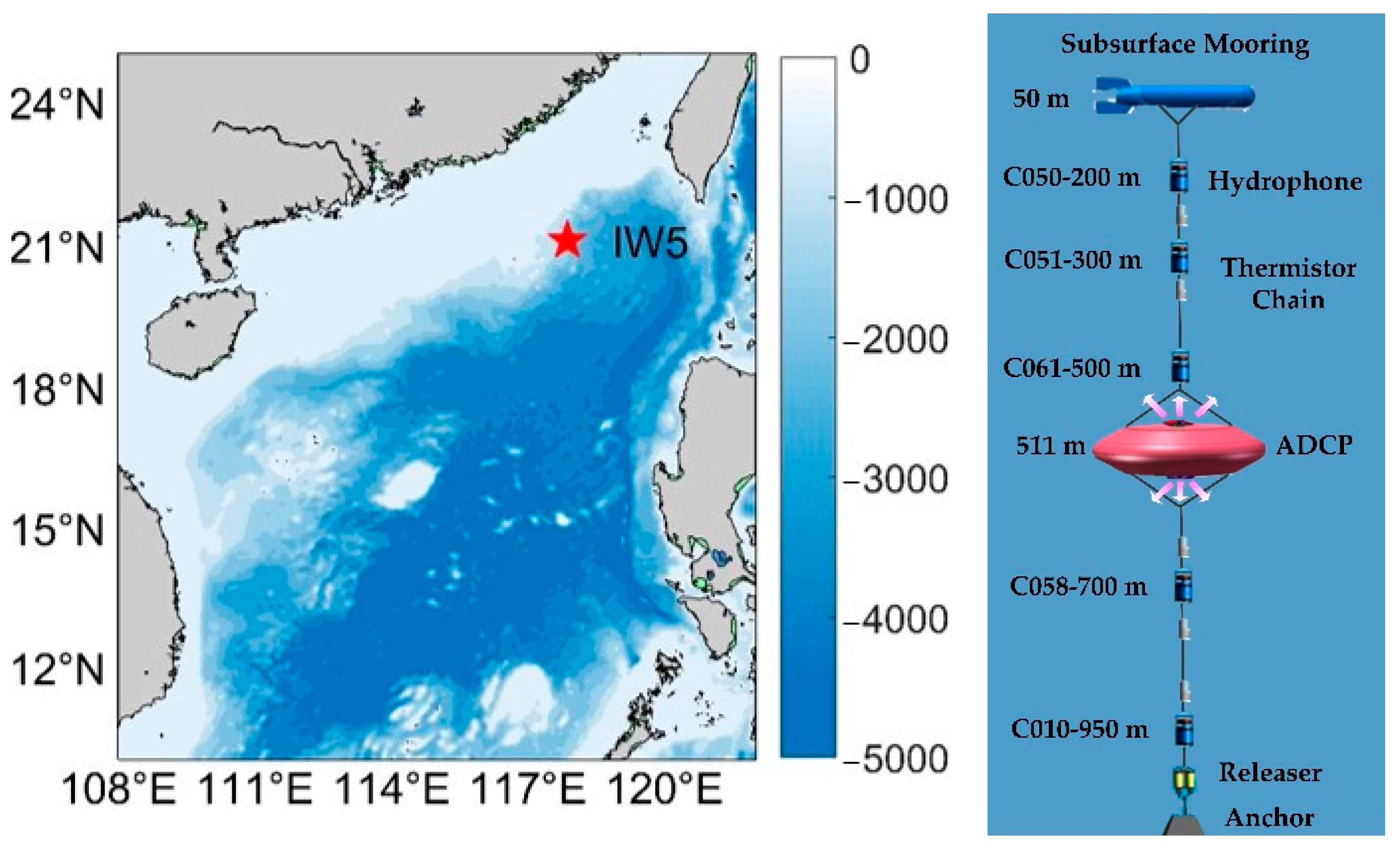
2. Experiment and Data

In this work, data were collected during the 2016 Internal Solitary Wave Cooperative Observation Experiment. The experiment was conducted in the north of the South China Sea from July 2016 to July 2017. Cooperative observation, consisting of oceanographic and acoustic instrumentation, was adopted in the experiment. A subsurface mooring system was deployed at a station labeled IW5 (117.87° E, 21.11° N) with a water depth of 1000 m, which was shown in Figure 1. Oceanographic data measured by thermistor chains and the acoustic doppler current profilers (ADCPs) were continuously observed. Both upward and downward-looking ADCPs were mounted on the mooring system at depth of 511 m in order to record flow velocity information. The temporal resolution was 3 min, and the vertical resolution was 16 m, covering a depth range of 110~850 m. The mooring system was equipped with thermistor chains of temperature loggers and Conductivity-Temperature-Depth (CTD) recorders between 110–930 m to collect temperature and salinity data. The temporal resolution was also 3 min.
The acoustic data were measured by a mooring-mounted hydrophone array attached on the cable. The array consisted of five independent acoustic hydrophones, spanning a depth of 200–950 m (Figure 1). The commercial hydrophones used on the array were independent acoustic hydrophones manufactured by the Institute of Acoustics of the Chinese Academy of Sciences. All hydrophones on the array were calibrated before experiment. Their received voltage responses were characterized. The sampling rate of the hydrophone was 4 kHz, and the sound pressure sensitivity of the hydrophone was −175 dB. The sensitivity value was fulfilled between 8 Hz to 2000 Hz without decaying more than −2 dB. Considering the storage and device power, the hydrophone was operated in intermittent mode (15 min every 3 h).
ISWs can cause large depressions on the isothermal surface and notable increases in the flow velocity. As shown in Figure 2, the duration time of temperature and velocity segments was 1 h, spanning a depth of 110−850 m. The influence time of ISWs on seawater temperature was about 15 min. The amplitudes of different ISWs varied greatly, from approximately 90 m to 160 m. The characteristic data for the three different ISWs focused in the study are shown in Table 1.
The mooring-mounted hydrophone array and thermistor chains were configured together. It took more than ten minutes for the internal wave to pass the mooring system, so we needed to find the noise data, with internal waves occurring and acoustic records, for analysis. In spite of the experiment period of one year, we only found a total of 6 events that matched the requirement, all of which were analyzed. Three with large internal wave amplitudes were selected for analysis, and the rest of the data also showed similar phenomena (Figure 2). Figure 3 depicts the data received by the C058 hydrophone at a depth of 700 m between 18:00 UTC+8 to 18:15 UTC+8 on 1 October 2016. Figure 3a shows the time-domain signal and the obvious noise burst when the internal wave arrived at 18:03 UTC+8. The time–frequency spectrum (Figure 3b) was obtained by short-time Fourier transform of the data. This analysis used a Hamming window of length 4096, with a 4096-point fast Fourier transform (FFT) and an overlap of 50%. The label of the time–frequency spectrum was power spectral density (PSD). Noise at about 500 Hz and some high frequency lines were generated by the shaking of the hydrophone and the collision of suspended particles in the water against the hydrophone casing when ISWs flowed past the mooring system.
It was notable that the low-frequency noise presented an identifiable frequency fluctuation at frequencies below 100 Hz, and the acoustic intensity increased with decreasing frequency. A further finding was that low-frequency noise had uniform harmonics, as depicted in Figure 3c (bright stripes). The generation mechanism for these features is discussed in the next section.

3. Analysis and Discussion of Noise Induced by Internal Solitary Waves

3.1. Korteweg-de Vries Equation Theory

The interfacial waves in an arbitrarily stratified fluid can be expressed by the classical Korteweg–de Vries (KdV) equation
η t + C 0 η x + α η η x + β 3 η x 3 = 0  
where η characterizes the vertical displacement of the isopycnal surface [15,29]. C 0 is a linear speed. The nonlinear parameter α and dispersion parameter β are considered environmental parameters and make contributions to density stratification and sheer currents [10].
In the two-layer fluid model, the upper layer has a thickness h 1 and a density ρ 1 , and the lower layer has a thickness h 2 and a density ρ 2 , and ρ 2 > ρ 1 [15]. This models a typical pycnocline. In this case, the linear speed is
C 0 = g h 1 h 2 δ ρ ρ a v ( h 1 + h 2 ) ,
where ρ a v = ( ρ 1 + ρ 2 ) / 2 is the mean density, δ ρ = ρ 2 ρ 1 is the density difference.
To illustrate the dynamics of a single wave packet of ISW in Figure 2, the solitary solution of KdV equation is
η = η 0 sech 2 x C p t l ,
where η 0 is the amplitude of the displacement, x is the horizontal position of an one-dimensional interfacial wave, and the nonlinear velocity C p and soliton width l [15,29].
C p = C 0 + α η 0 3 ,   l = 12 β α η 0  
The nonlinear and dispersion parameters ( α and β ) of the model are
α = 3 C 0 ( h 1 h 2 ) 2 h 1 h 2 ,   β = C 0 h 1 h 2 6 .  
Using the explicit form of environmental parameters α and β , Equation (4) becomes
C p = [ 1 + η 0 ( h 1 h 2 ) 2 h 1 h 2 ] ,   l = 2 h 1 h 2 3 η 0 | h 1 h 2 | .
This solitary solution is the typical characteristic of ISW in many areas of the ocean [15].

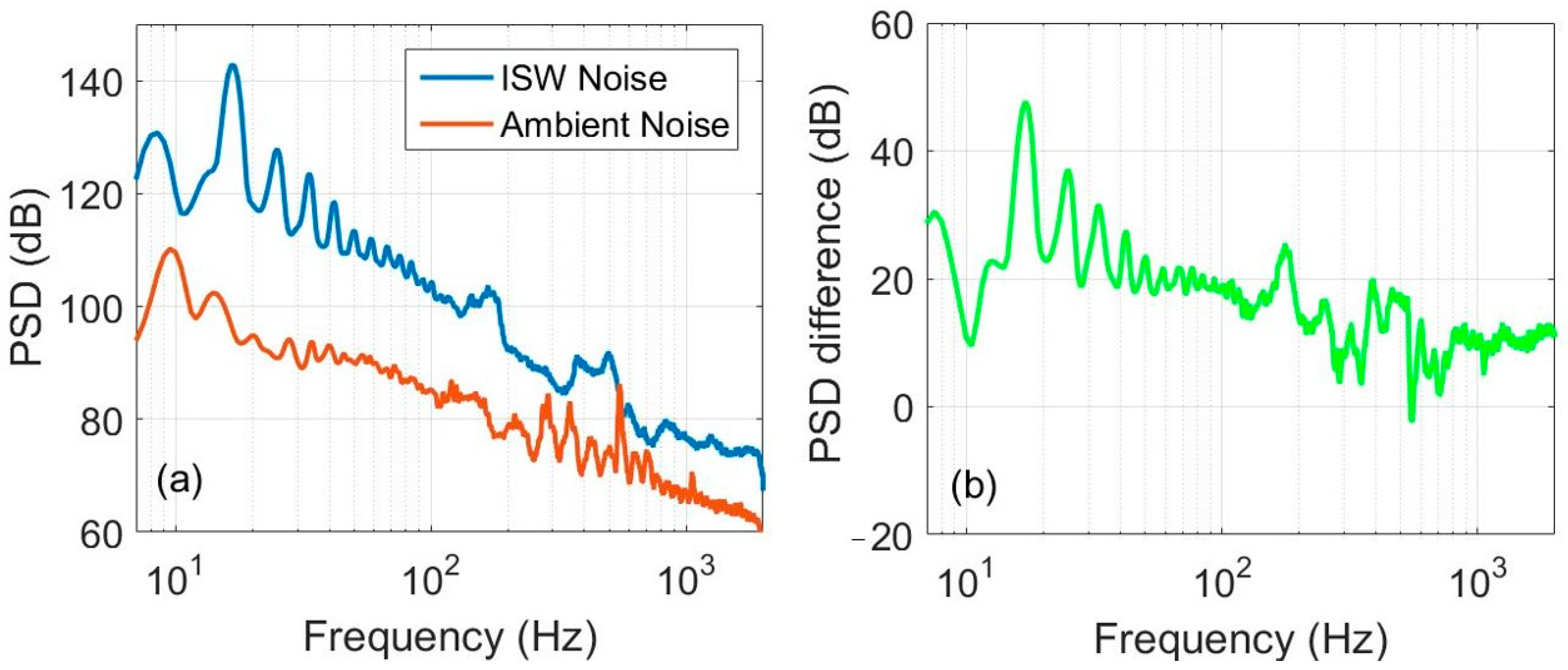
3.2. Spectra Comparison of ISW Noise and Ambient Noise

This section served to illustrate the effects of ISW noise on the ambient noise. Figure 4a shows the power spectra of the noise received by the hydrophone located at 700 m during the passage of internal waves and the ambient noise received three hours later (from 9:00 to 9:02 UTC+8). The data duration was 2 min. The differences in PSD between the two PSD curves are shown in Figure 4b. The spectral level of ISW noise was about 20–40 dB higher than that of ambient noise at frequencies between 10 Hz and 50 Hz. Due to the effects of low frequency harmonics, the maximum difference was 47.7 dB. As the frequency increased, the spectral level gap narrowed. Up to 2 kHz, the difference remained around 10 dB. Flow noise was the dominant source below 100 Hz. Distant ships may be responsible for the peaks in the ambient noise between 200 Hz and 500 Hz. The noise comparison revealed that the ambient noise was completely drowned out by the ISW noise below 2 kHz.

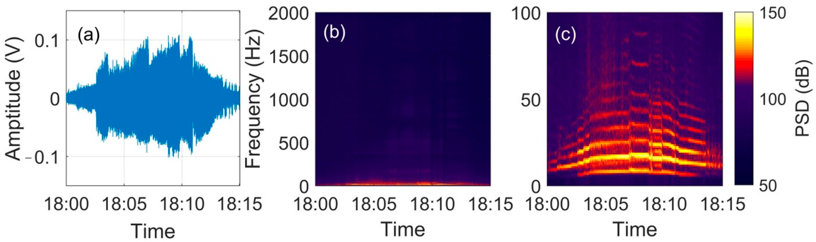
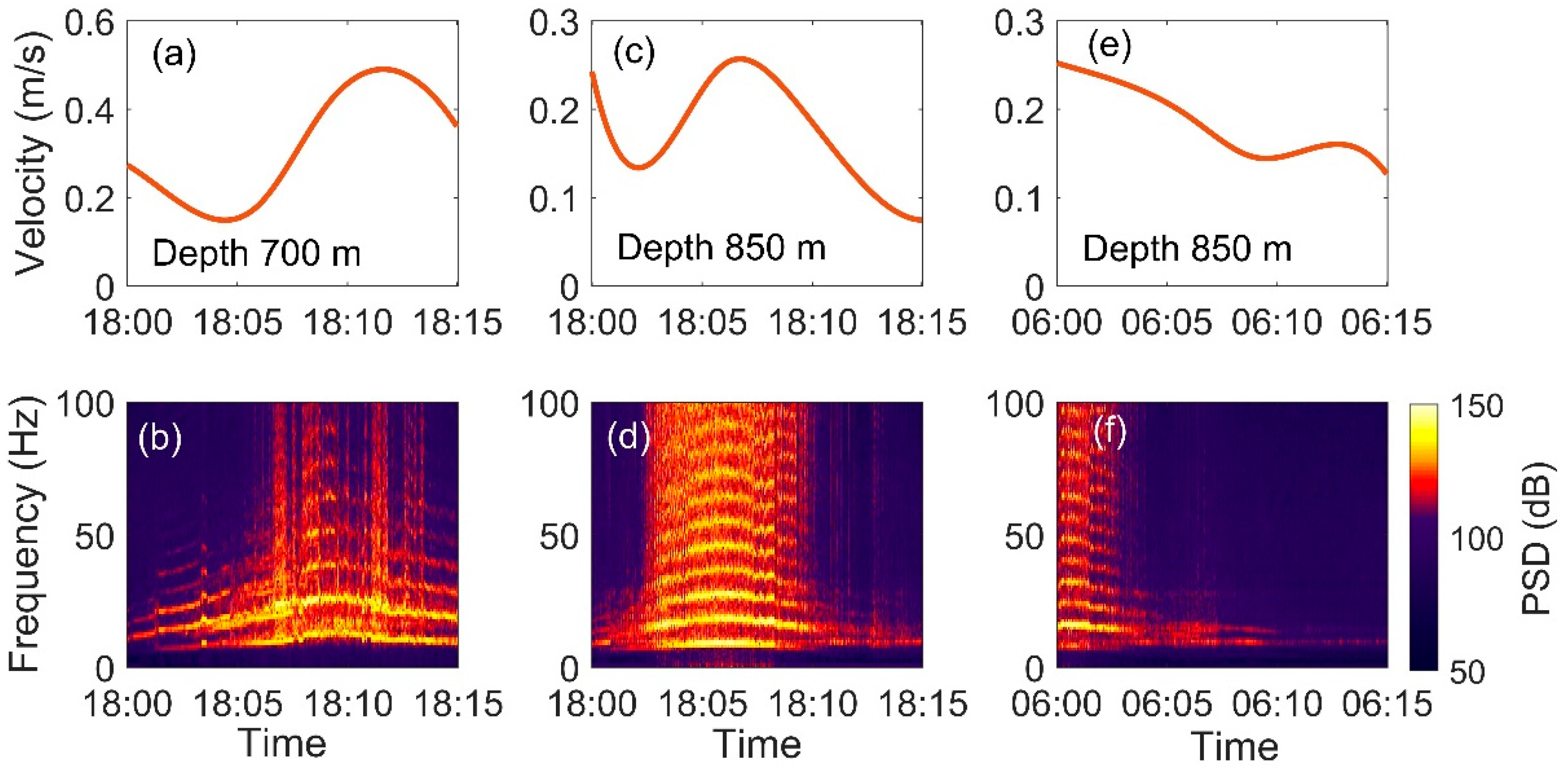
3.3. Low-Frequency Noise Induced by ISWs

3.3.1. Relationship between Low-Frequency Noise and ISWs

We interpreted the observed low-frequency noise as the flow noise induced by ISWs [23,27]. For this purpose, we analyzed data collected from other ISWs. Figure 5 shows the time–frequency spectra of low frequency noise and their corresponding flow velocities (The data time is consistent with Table 1). The increase in flow velocity was almost synchronous with the burst of low frequency noise. The noise on 21 September 2016 was incomplete, as the maximum velocity occurred at 5:54 UTC+8. As discussed, these results were in accordance with the properties of flow noise induced by ISWs.
It was interesting to note that each segment of noise induced by the ISWs had fundamental and harmonic waves. To elucidate the characteristics of the harmonic waves, we used a 16.384 s data block with 50% overlap (65536-points FFT) from the center of each signal for spectrum analysis. The Welch method and Blackman window were used to calculate power spectra. Figure 6 shows the power spectra corresponding to the three signals in Figure 5. Table 2 shows their fundamental and harmonic frequencies. Each segment of signal had a different fundamental frequency. This phenomenon may be associated with the velocity of the ISW. It was worth discussing these facts, in terms of which part of the mooring system the internal wave interacted with, to produce low-frequency flow noise and harmonics.

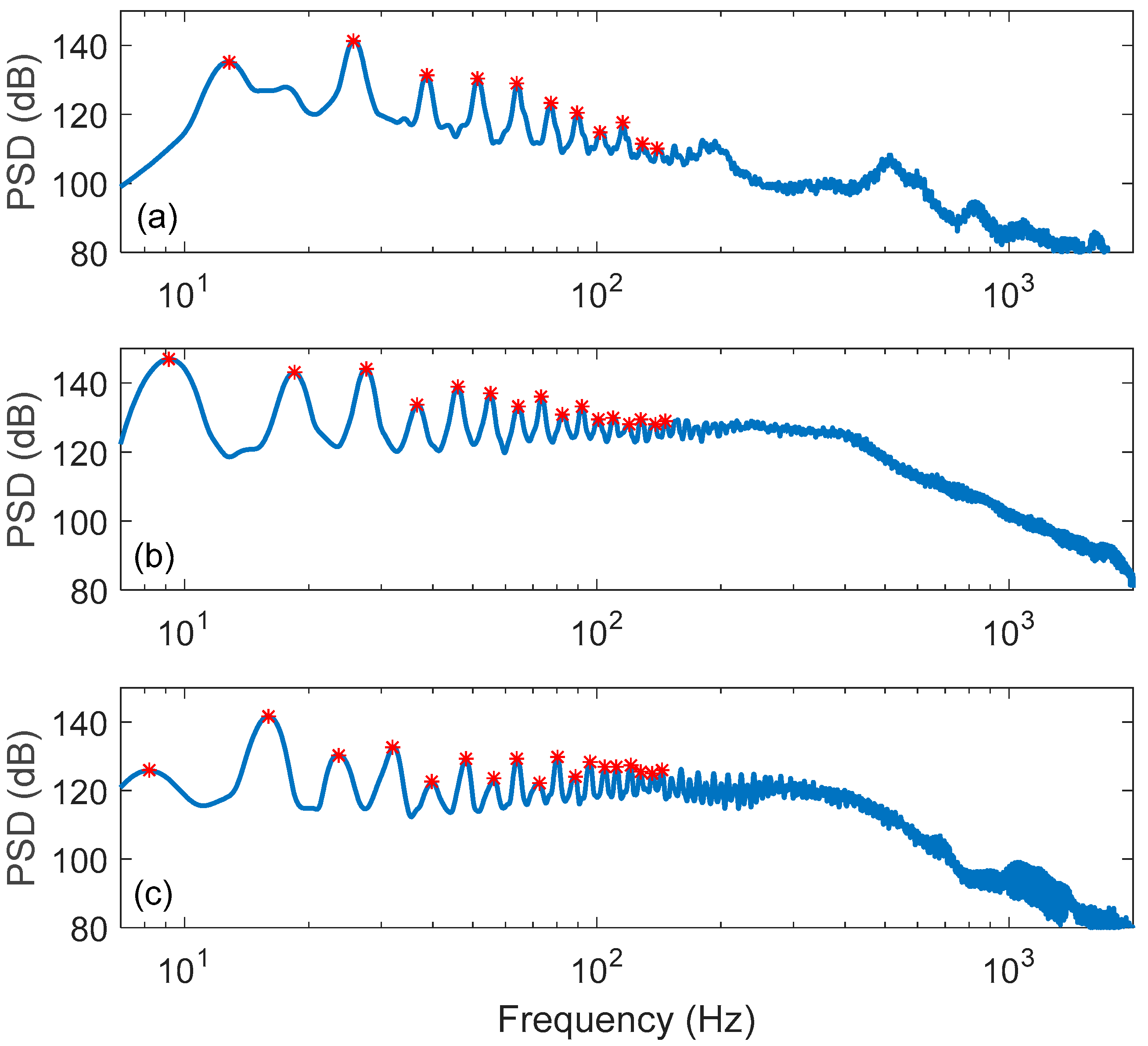
3.3.2. Vortex-Induced Vibration

The cable of the mooring system can be abstracted as a flexible riser in the water with the upper end subjected to vertical tension and the lower end fixed. The current, when flowing past the cylinder, generates a vortex alternately, therefore, periodic pressure changes occur around the cylinder [30]. When the cylinder is a flexible structure, the periodic vibration of the cylinder structure is caused by the alternating pressure, namely vortex-induced vibration [30]. This can be used to account for the vibration caused by internal waves flowing past the cable system.
As far as we know, little previous research has investigated the VIV induced by ISWs. However, VIV produced by other kinds of currents around a cylinder has been widely documented. In 1911, Karman conducted a pioneering study on vortex shedding around the flow based on the non-viscous method. When a viscous fluid passes through a cylindrical structure, its wake will undergo flow separation and form two rows of vortices alternately, which is called a Karman vortex street [31]. When the frequency of the vortex is close to the natural frequency of the structure, structural resonance or VIV occurs. Kassen [32], Sarpkaya [33] and Wu [34] provided detailed explanations of VIV, including generation mechanism, models, wake form, self-locking phenomenon and so on.
Although there have been many studies of VIV on underwater flexible risers in the laboratory, there have been few underwater experimental studies owing to the high cost of full-scale field experiments. Large-scale model tests of tensioning risers (90 m in length and 3 cm in diameter) were carried out in a lake on Norway’s west coast in 1997 [35]. Lie used modal analysis to determine that the VIV was irregular in the non-lock-incase, and that the vibration frequency was composed of the natural frequency of the structure plus the frequency of vortex shedding along the length of the structure [35]. Recent studies have shown that the VIV of the flexible riser had multi-order harmonics. Wu determined that higher harmonics could be present with flexible beam VIV [36]. Trim analyzed the second harmonic frequency component of the VIV from a flexible riser (38 m in length and 2.7 cm in diameter) in the Marintek Ocean Basin in Trondheim [37]. When Wang analyzed the multi-order modes and harmonics of the cable-coupled vibration response, he found that, the closer to the midpoint of the cable, the higher the excitation degree of the first two modes, and the farther away from the midpoint of the cable, the more average the excitation degree of the first six modes. [38]. The uniform harmonic component was evidence of internal wave noise. This was also consistent with the results of our analysis in Figure 6. It was considered that the oscillations of the marine cables system would cause noise in the sonar system, reducing the performance of other environmental sensors [30].
When uniform turbulence flows past a rigid, fixed riser of diameter d, the time-varying motion of the riser can be made up of a series of mode-shapes if the dynamical process of the riser vibration is approximately linear [35].
x ( t , z ) = n = 1 w n ( t ) φ n ( z ) ,   z [ 0 , L ] ,  
where L is the length of the riser, z is the vertical coordinate, and t is the time. The horizontal displacement of the riser x(t,z) is determinded by the mode-shape φ n ( z ) and the modal weight w n ( t ) , n = 1, 2, 3… [35].
The vortex shedding frequency is
f V I V = S t u / d ,
where the u is the free-current velocity. When the cable diameter is no more than 0.1 m, the maximum Reynolds number for the mooring system is usually less than 105, and during a wide range of the Reynolds number (Re), 102 < Re < 105, the Strouhal number (St) varies little and has a value around 0.2 [30,35].
We knew the diameter of the cable (1 cm) and the velocity at the depth of the hydrophones at different times. The vortex shedding frequency was consistent with the structural natural frequency [30]. The shedding frequency was calculated using Equation (8). As shown in Table 3, shedding frequency was positively correlated with the ISW velocity. The velocity increased as the internal wave approached the hydrophone and decreased as the internal wave moved away from the hydrophone. Therefore, the frequency of the noise appearred to increase first and then decrease, appearing as a frequency fluctuation in the time–frequency spectra.
The fundamental frequencies (Table 2) of the noise with maximum spectra at 18:09, 18:06 and 06:00 UTC+8 were 12.72 Hz, 9.16 Hz and 8.18 Hz, respectively. The actual frequency was higher than the calculated frequency. The vibration of the cable depended not only on the velocity of the internal waves, but also on the mass of the cable, the added mass, the elasticity and the damping coefficient [35]. Locking and synchronization may occur if the natural resonant frequency of the cable approximates the Strouhal frequency [30]. In this case, the vortex fell off at the actual frequency, not the frequency calculated by Equation (8), because the formation and shedding process of the vortex changed the added mass of the cable [30,35]. The change in added mass may be positive or negative, causing an increase or decrease in shedding frequency [35]. In addition, the velocity of ISW varied greatly with time and space, further complicating the vortex shedding frequency [38].
Together, the characteristics and frequency components of the VIV were consistent with our analysis of flow noise. The results of the experiment found clear support for low frequency noise induced by VIV when ISWs flowed past the marine cable system.

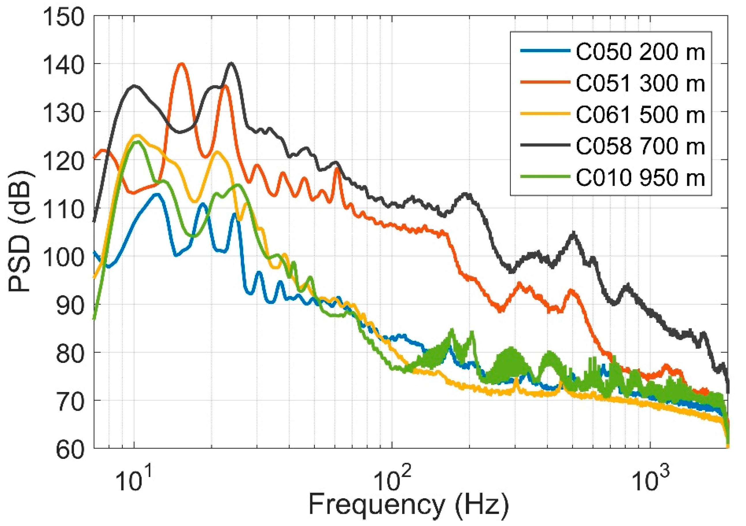
3.4. Spectrum Comparison of ISW Noise at Different Depths

To illustrate the depth dependence of ISW noise, Figure 7 shows the power spectra comparison as a function of the frequency for five hydrophones at depths of 200 m, 300 m, 500 m, 700 m, and 950 m. As shown in Figure 7, the distant noise component below 100 Hz was derived from the flow noise induced by ISWs. The fundamental frequencies of the noise differed substantially because of the velocity difference of internal waves at different depths.
The noise spectrum levels of the hydrophones at 200 m, 500 m, and 700 m were less than those at 300 m and 700 m. The key was the structure of the entire mooring system. The vibration amplitude of the cable decreased with the increase of tension [38,39]. The hydrophone, C050, at 200 m, was close to the main floater at the top of the cable system. Hydrophone C061, at 500 m, approached the central floater where the ADCPs were located. Hydrophone C010, at 950 m, was located near the fixed object at the bottom of the cable. Hydrophone C058 had a larger spectrum level than hydrophone C051, because the floater at 500 m divided the cable into two sections, shorter at the top and longer at the bottom. The longer the vibration length of the cable, the greater the vibration amplitude [39].

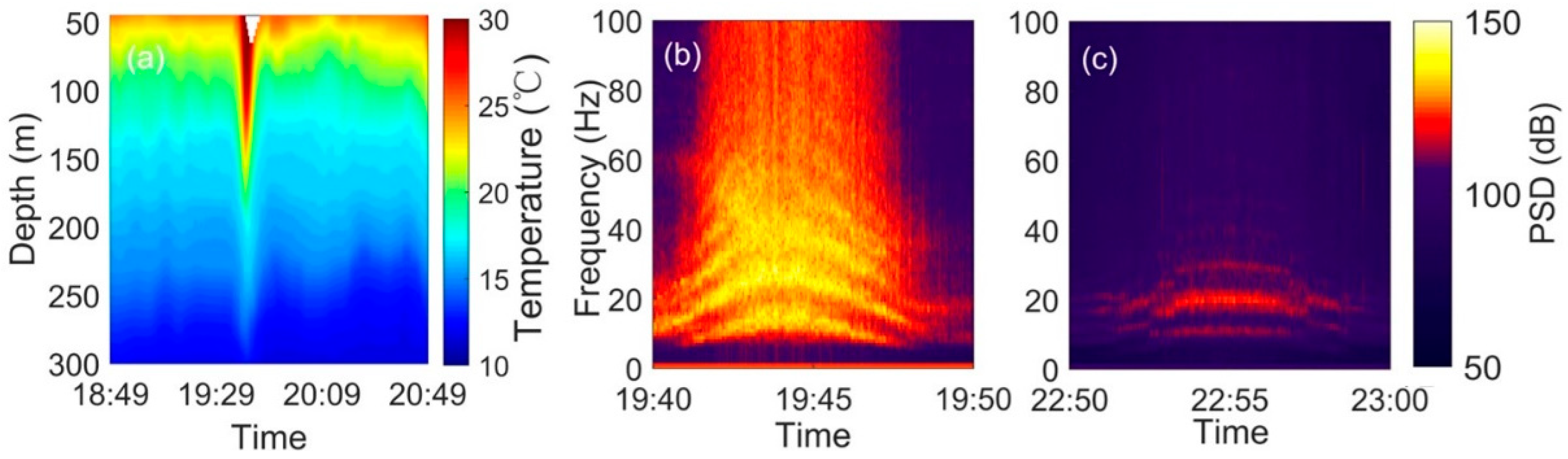
4. Comparison of ISW Noise in 2019 ISW Observation Experiment

This section compares noise measurements from the 2019 Internal Solitary Wave Observation Experiment. The experiment was located on the continental shelf of the South China Sea with an average water depth of 360 m.
Figure 8 shows the temperature data and the noise of the same internal wave received by two hydrophones. The maximum amplitude of this ISW was 91.74 m which arrived at 19:42 UTC+8. Figure 8b shows the time–frequency spectrum below 100 Hz recorded by a hydrophone located at depth of 200 m, which was the middle hydrophone of the mooring-mounted linear array. The length of the cable in this experiment was about 300 m. The fundamental frequency of low frequency noise was 10.20 Hz, with uniform harmonic components.
The results confirmed that the flow noise induced by ISWs was indeed caused by the VIV of the cable system. The noise in Figure 8c was from the near-bottom hydrophone at a depth of 340 m, 17.8 km west of the mooring-mounted linear array. The length of the cable that held the hydrophone was 30 m. When the same ISW flowed past the near-bottom hydrophone, the noise intensity was substantially reduced. The fundamental frequency of low frequency noise was 6.15 Hz.
A comparison between ISW observations in the 2016 experiment and the 2019 experiment is shown in Table 4. The amplitude of the internal wave in the 2019 experiment was slightly smaller than that observed in the 2016 experiment. Due to the shallow sea, the cable length of the mooring system was much smaller than that of the deep-sea experiment. This result showed that the noise intensity induced by ISW was related to the cable length, because the longer the cable, the stronger the VIV [30,35]. This was also related to the position of the hydrophone attached on the mooring system. Overall, all noise datasets had uniform harmonics, which was in accordance with the characteristics of flow velocity.

5. Conclusions

In this study, oceanographic and acoustic data from the 2016 Internal Solitary Wave Cooperative Observation Experiment in the South China Sea were studied. We analyzed the noise during three large ISWs and found that ISWs produced strong noise at low frequencies. The analysis results could be used as a supplement to internal wave observations and provide a passive acoustic monitoring and warning method for high marine currents.
Within 15 min of the internal wave flowing past the subsurface mooring, the isothermal surface was depressed substantially, with a maximum amplitude reaching 160 m and the maximum velocity exceeding 2 m/s. The noise received by the mooring-mounted hydrophone array also increased.
Compared with the ambient noise, the results indicated that the ISW noise was higher than the ambient noise at frequencies below 2 kHz, and even higher than 20–40 dB within 100 Hz.
Through analysis of time–frequency spectra and power spectra, we interpreted the low frequency noise as vortex-induced vibration caused by ISWs flowing past the marine cable system owing to the significant harmonic component of the noise. The noise duration was basically consistent with the time of ISWs interacting with the mooring system. It was notable that the frequency fluctuation of noise was caused by the variation of internal wave velocities with time and space. Through comparison of the ISW noises received by hydrophones at different depths, we found that the power spectra of ISW noises were associated with the positions of the hydrophones fixed on the cable. The closer to the fixed end, the smaller the noise spectrum level, and vice versa.
For further evidence, the observation experiment of internal waves in the South China Sea in 2019 confirmed that the frequency fluctuation and harmonic components of low frequency noise induced by internal solitary waves still occurred under different experimental conditions.
The results of this study could establish a high marine current warning and real-time marine current monitoring system, because the observed acoustic characteristics, including harmonics, frequency fluctuation, and energy enhancement, were intrinsically related to the velocity and amplitude of internal waves. Oceanographic phenomena can be studied based on acoustic observations and noise analysis. In addition, when studying oceanographic phenomena, acoustic signal analysis technology can receive data through a single hydrophone on the mooring system, without the full ocean depth thermistor chains and ADCP. It would be both cheaper and more practical than other ocean instruments.
To our knowledge, few studies have examined the model of the marine cable system vibration under ISWs. Therefore, the low frequency noise induced by ISWs calls for further experimentation and theoretical exploration.

Author Contributions

Conceptualization, J.L. and Y.S.; methodology, J.L. and Y.S.; formal analysis, J.L., Y.S., Y.Y. and X.H.; resources, Y.S. and X.H.; data curation, J.L.; writing—original draft preparation, J.L.; writing—review and editing, J.L., Y.S., Y.Y. and X.H.; supervision, Y.Y.; funding acquisition, Y.S. and Y.Y. All authors have read and agreed to the published version of the manuscript.

Funding

This research was funded by the National Natural Science Foundation of China, grant number 41906160, 11974286, 12174312.

Institutional Review Board Statement

Not applicable.

Informed Consent Statement

Not applicable.

Data Availability Statement

The data from 2016 Internal Solitary Wave Cooperative Observation Experiment presented in this study are available on request from the corresponding author.

Acknowledgments

We are grateful to Bingyong Guo for providing helpful suggestions about VIV in the manuscript.

Conflicts of Interest

The authors declare no conflict of interest.

References

  1. Helfrich, K.R.; Melville, W.K. Long Nonlinear Internal Waves. Ann. Rev. Fluid Mech. 2006, 38, 395–425. [Google Scholar] [CrossRef]
  2. Osborne, A.; Burch, T. Internal solitons in the Andaman Sea. Science 1980, 208, 451–460. [Google Scholar] [CrossRef] [PubMed]
  3. Jackson, C. Internal wave detection using the Moderate Resolution Imaging Spectroradiometer (MODIS). J. Geophys. Res. 2007, 112, C10012. [Google Scholar] [CrossRef] [Green Version]
  4. Zhang, S.; Alford, M.H.; Mickett, J.B. Characteristics, generation and mass transport of nonlinear internal waves on the Washington continental shelf. J. Geophys. Res. Oceans 2015, 120, 741–758. [Google Scholar] [CrossRef]
  5. Scotti, A.; Beardsley, R.C.; Butman, B. Generation and propagation of nonlinear internal waves in Massachusetts Bay. J. Geophys. Res. 2007, 112, C10001. [Google Scholar] [CrossRef]
  6. Lee, S.W.; Nam, S. Estimation of Propagation Speed and Direction of Nonlinear Internal Waves from Underway and Moored Measurements. J. Mar. Sci. Eng. 2021, 9, 1089. [Google Scholar] [CrossRef]
  7. Huang, X.; Chen, Z.; Zhao, W.; Zhang, Z.; Zhou, C.; Yang, Q.; Tian, J. An extreme internal solitary wave event observed in the northern South China Sea. Sci. Rep. 2016, 6, 30041. [Google Scholar] [CrossRef] [Green Version]
  8. Ramp, S.R.; Tang, T.Y.; Duda, T.F.; Lynch, J.F.; Liu, A.K.; Chiu, C.S.; Bahr, F.L.; Kim, H.R.; Yang, Y.J. Internal Solitons in the Northeastern South China Sea Part I: Sources and Deep Water Propagation. J. Ocean. Eng. 2004, 29, 1157–1181. [Google Scholar] [CrossRef]
  9. Xu, A.; Chen, X. A Strong Internal Solitary Wave with Extreme Velocity Captured Northeast of Dong-Sha Atoll in the Northern South China Sea. J. Mar. Sci. Eng. 2021, 9, 1277. [Google Scholar] [CrossRef]
  10. Cai, S.; Xie, J.; He, J. An overview of internal solitary waves in the South China Sea. Surv. Geophys. 2012, 33, 927–943. [Google Scholar] [CrossRef]
  11. Colosi, J.A.; Scheer, E.K.; Flatte, S.M.; Cornuelle, B.D.; Dzieciuch, M.A.; Munk, W.H.; Worcester, P.F.; Howe, B.M.; Mercer, J.A.; Spindel, R.C.; et al. Comparisons of measured and predicted acoustic fluctuations for a 3250-km propagation experiment in the eastern North Pacific Ocean. J. Acoust. Soc. Am. 1999, 105, 3202–3218. [Google Scholar] [CrossRef]
  12. Katsnelson, B.G.; Godin, O.A.; Zhang, Q. Observations of acoustic noise bursts accompanying nonlinear internal gravity waves on the continental shelf off new jersey. J. Acoust. Soc. Am. 2021, 149, 1609–1622. [Google Scholar] [CrossRef]
  13. Simmen, J.; Flatte, S.M.; Wang, G.Y. Wavefront folding, chaos, and diffraction for sound propagation through ocean internal waves. J. Acoust. Soc. Am. 1997, 102, 239–255. [Google Scholar] [CrossRef]
  14. Katsnelson, B.G.; Grigorev, V.; Badiey, M.; Lynch, J.F. Temporal sound field fluctuations in the presence of internal solitary waves in shallow water. J. Acoust. Soc. Am. 2009, 126, EL41–EL48. [Google Scholar] [CrossRef] [Green Version]
  15. Apel, J.R.; Ostrovsky, L.A.; Stepanyants, Y.A.; Lynch, J.F. Internal solitons in the ocean and their effect on underwater sound. J. Acoust. Soc. Am. 2007, 121, 695–722. [Google Scholar] [CrossRef]
  16. Badiey, M.; Mu, Y.; Lynch, J.; Apel, J.; Wolf, S. Temporal and azimuthal dependence of sound propagation in shallow water with internal waves. IEEE J. Ocean. Eng. 2002, 27, 117–129. [Google Scholar] [CrossRef]
  17. Tang, D.; Moum, J.N.; Lynch, J.F.; Abbot, P.; Chapman, R.; Dahl, P.H.; Duda, T.F.; Gawarkiewicz, G.; Glenn, S.; Goff, J.A.; et al. Shallow Water ‘06: A joint acoustic propagation/nonlinear internal wave physics experiment. Oceanography 2007, 20, 156–167. [Google Scholar] [CrossRef] [Green Version]
  18. Wei, R.C.; Chien, K.F.; Chiu, L.; Chen, C.F. Analysis of low frequency ocean ambient noise induced by internal wave in sand dune region of northern South China Sea. J. Acoust. Soc. Am. 2016, 140, 3013. [Google Scholar] [CrossRef]
  19. Serebryany, A.N.; Newhall, A.; Lynch, J.F. Observations of noise generated by nonlinear internal waves on the continental shelf during the SW06 experiment. J. Acoust. Soc. Am. 2008, 123, 3589. [Google Scholar] [CrossRef] [Green Version]
  20. Yang, Y.J.; Chiu, C.S.; Wu, J.C.; Liang, W.D.; Ramp, S.R.; Reeder, D.B.; Chen, C.F. Observations of ambient noises induced by the internal solitary waves on the continental slope of the northern South China Sea: Ambient noises by ISW in SCS. In Proceedings of the OCEANS 2015-Genova, Genova, Italy, 21 September 2015; pp. 1–4. [Google Scholar]
  21. Bassett, C.; Thomson, J.; Polagye, B.L. Sediment-generated noise and bed stress in a tidal channel. J. Geophys. Res. Oceans 2013, 2249–2265. [Google Scholar] [CrossRef]
  22. Bourgault, D.; Morsilli, M.; Richards, C.; Neumeier, U.; Kelley, D.E. Sediment resuspension and nepheloid layers induced by long internal solitary waves shoaling orthogonally on uniform slopes. Cont. Shelf Res. 2014, 72, 21–33. [Google Scholar] [CrossRef] [Green Version]
  23. Bassett, C.; Thomson, J.; Dahl, P.H.; Polagye, B. Flow-noise and turbulence in two tidal channels. J. Acoust. Soc. Am. 2014, 135, 1764–1774. [Google Scholar] [CrossRef] [Green Version]
  24. Dietz, F.T.; Kahn, J.S.; Birch, W.R. Nonrandom associations between shallow water ambient noise and tidal phase. J. Acoust. Soc. Am. 1960, 32, 915. [Google Scholar] [CrossRef]
  25. Willis, J.; Dietz, F.T. Some characteristics of 25-cps shallow-water ambient noise. J. Acoust. Soc. Am. 1965, 37, 125–130. [Google Scholar] [CrossRef]
  26. Deane, G.B. Long time-base observations of surf noise. J. Acoust. Soc. Am. 2000, 107, 758–770. [Google Scholar] [CrossRef]
  27. Strasberg, M. Non-acoustic noise interference in measurements of infrasonic ambient noise. J. Acoust. Soc. Am. 1979, 66, 1487–1493. [Google Scholar] [CrossRef]
  28. Webb, S.C. Long-period acoustics and seismic measurements and ocean floor currents. J. Ocean. Eng. 1988, 13, 263–270. [Google Scholar] [CrossRef]
  29. Gerkema, T. An Introduction to Internal Waves; Lecture Notes; Royal NIOZ: Texel, The Netherlands, 2008; pp. 147–164. [Google Scholar]
  30. Every, M.J.; King, R.; Weaver, D.S. Vortex-excited vibrations of cylinders and cables and their suppression. Ocean Eng. 1982, 9, 135–157. [Google Scholar] [CrossRef]
  31. Pankanin, G.L.; Kulińczak, A.; Berliński, J. Investigations of Karman vortex street using flow visualization and image processing. Sensors Actuat. Phys. 2007, 138, 366–375. [Google Scholar] [CrossRef]
  32. Kaasen, K.E.; Lie, H.; Solaas, F.; Vandiver, J.K. Norwegian Deepwater Program: Analysis of Vortex-Induced Vibrations of Marine Risers Based on Full-Scale Measurements. In Offshore Technology Conference; OTC Program Committee: Houston, TX, USA, 2000; p. OTC-11997-MS. [Google Scholar]
  33. Sarpkaya, T. Hydrodynamic damping, flow-induced oscillations, and biharmonic response. J. Offshore Mech. Arct. Eng. 1995, 117, 232–238. [Google Scholar] [CrossRef]
  34. Wu, J.; Yin, D.; Halvor, L. On the occurrence of higher harmonics in the VIV response. In OMAE 2015 34th International Conference; AMSE: St. John’s, NL, Canada, 2015; p. OMAE2015-42061. [Google Scholar]
  35. Lie, H.; Kaasen, K.E. Modal analysis of measurements from a large-scale VIV model test of a riser in linearly sheared flow. J. Fluid. Struct. 2006, 22, 557–575. [Google Scholar] [CrossRef]
  36. Trim, A.D.; Braaten, H.; Lie, H.; Tognarelli, M.A. Experimental investigation of vortex-induced vibration of long marine risers. J. Fluid. Struct. 2005, 21, 335–361. [Google Scholar] [CrossRef]
  37. Wang, J.X.; Gui, H.B.; Chen, X. Analysis of Attitude and Dynamics Characteristic of a Kind of Submerged Buoy. Appl. Mech. Mater. 2012, 226, 516–520. [Google Scholar] [CrossRef]
  38. Hover, F.S.; Miller, S.N.; Triantafyllou, M.S. Vortex-induced vibration of marine cables: Experiments using force feedback. J. Fluid. Struct. 1997, 11, 307–326. [Google Scholar] [CrossRef]
  39. Owen, M.G.; Richard, A.S.; Steven, E.R. The Resonant, Vortex-Excited Vibrations of structures and Cable Systems. In Offshore Technology Conference; OTC Program Committee: Houston, TX, USA, 1975; p. OTC-2319-MS. [Google Scholar]
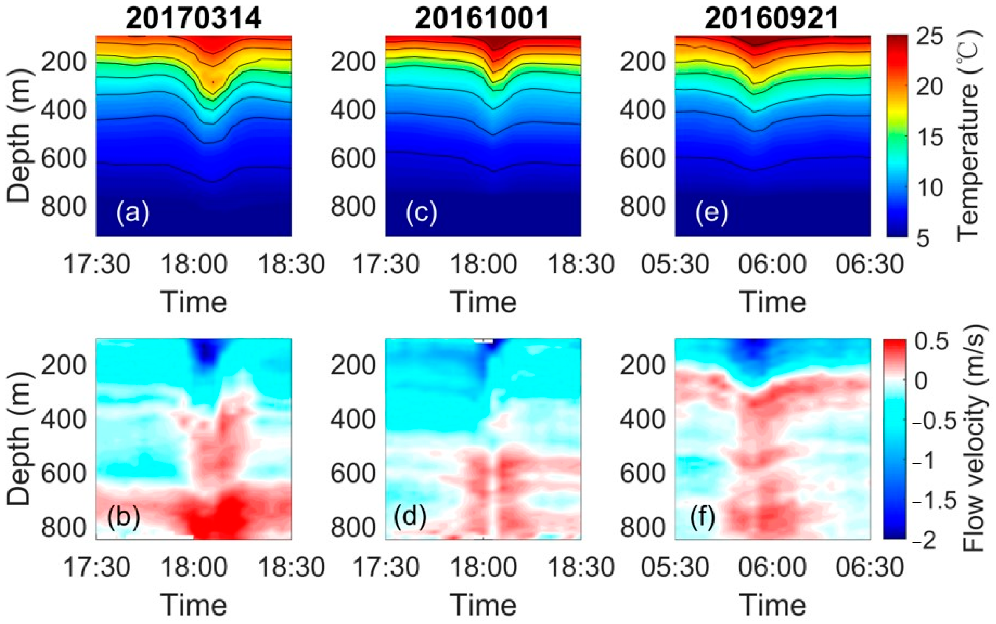
Figure 1. The topography in the South China Sea. The red pentagram indicates the location of the experimental site (IW5 station). The right figure shows the subsurface mooring system.
Jmse 10 00222 g001
Figure 2. Temperatures and flow velocities for ISWs passing by the IW5 station on three different days. (a,c,e) Temperatures measured by thermistor chains. (b,d,f) Flow velocities measured by the ADCPs. The flow velocity from west to east is positive and the reverse is negative. The flow velocity in this work refers to the zonal velocity. All data sampled at UTC+8.
Jmse 10 00222 g002
Figure 3. The signal received by the C058 hydrophone at a depth of 700m from 18:00 UTC+8 to 18:15 UTC+8 on 1 October 2016. (a) Time–domain signal. (b) Time–frequency spectrum. (c) Time–frequency spectrum between 0 Hz and 100 Hz.
Jmse 10 00222 g003
Figure 4. Power spectrum comparison of ISW noise and ambient noise. (a) PSD comparison. (b) The differences of PSD between ISW noise and ambient noise. ISW noise is from the 2 min data received by hydrophone C058 at depth of 700 m between 6:00 to 6:02 UTC+8 on 21 September 2016, and the ambient noise is from data three hours later (from 9:00 to 9:02 UTC+8).
Jmse 10 00222 g004
Figure 5. Flow velocities and time–frequency spectra (dB) of the C058 hydrophone (700 m) on (a,b) 14 March 2017. Flow velocities and time–frequency spectra of the C010 hydrophone (950 m) on (c,d) 1 October 2016 and (e,f) 21 September 2016. The depth on the figures represents the depth at which the flow velocity was measured.
Jmse 10 00222 g005
Figure 6. Power spectra of the noise recorded by the same hydrophones as in Figure 5. (a) The data after 18:09 UTC+8. (b) The data after 18:06 UTC+8. (c) The data after 6:00 UTC+8. The data length is 16.384 s.
Jmse 10 00222 g006
Figure 7. Power spectra comparison of ISW noise from five hydrophones at different depths from 18:06 to 18:08 UTC+8 on 14 March 2017.
Jmse 10 00222 g007
Figure 8. Temperature data and noise of the same ISW received by two hydrophones on 9 July 2019. (a) Temperature measured by the thermistor chains. (b) Time–frequency spectrum from a hydrophone at a depth of 250 m. The cable of the hydrophone array is 300 m long. (c) Time–frequency spectrum from the near–bottom hydrophone at a depth of 340 m. The cable of the single hydrophone is 30 m long.
Jmse 10 00222 g008
Table 1. Characteristic data for ISWs on three different days.
Observation DateTime (UTC+8)Max AmplitudeMax Flow Velocity
2017031418:06159.65 m−2.09 m/s
2016100118:03118.28 m−1.78 m/s
2016092105:5498.30 m−1.52 m/s
Table 2. The fundamental and harmonic frequencies of the three signals (Hz).
FundamentalDoubleTripleQuadrupleFive-TimesSix-TimesSeven-TimesEight-Times
12.7225.3939.0651.7664.6577.1589.84105.32
9.1618.4327.5936.7445.8955.0564.5873.49
8.1816.1124.1732.3540.4148.5856.5264.58
Table 3. ISW velocities and calculated frequencies of the hydrophones at different times.
HydrophoneC058-20170314 (700 m)C010-20161001 (950 m)C010-20160921 (950 m)
Time18:0318:0918:0318:0606:0006:03
Velocity (cm/s)41.8252.9021.7425.2623.6217.11
Frequency (Hz)8.3610.584.355.054.723.42
Table 4. The comparison between ISW observations in the 2016 experiment and 2019 experiment.
2019 Experiment2016 Experiment
Water depth (m)360 m1000 m
Cable length (m)300 m30 m490 m490 m490 m
Amplitude of ISW (m)91.74 m91.74 m159.65 m118.28 m98.30 m
Hydrophone locationmiddlebottommiddlebottombottom
Fundamental frequency (Hz)10.20 Hz6.15 Hz12.72 Hz9.16 Hz8.18 Hz
Publisher’s Note: MDPI stays neutral with regard to jurisdictional claims in published maps and institutional affiliations.

