Abstract
Agricultural green development is an essential pathway to achieving comprehensive agricultural and rural modernization and holds significant importance for ensuring national food, resource, and ecological security. Based on panel data from 30 provinces in China during 2004–2022, this study employed the super-efficiency SBM-GML model, the modified gravity model, social network analysis (SNA), and the quadratic assignment procedure (QAP) regression model to systematically analyze the spatial association network characteristics and driving mechanisms of agricultural green development in China. The results showed that (1) the number of spatial linkages in interprovincial agricultural green development had been increasing, with the network exhibiting strong connectivity, stability, and accessibility. (2) Major grain-producing areas and economically developed regions along the eastern coast had become the driving sources of spatial spillovers in agricultural green development. Meanwhile, the central and western regions acted as “brokers” in facilitating the reception and transfer of resources within the overall network, while municipalities such as Tianjin and Shanghai exhibited siphon effects on other regions. (3) Geographical proximity, government fiscal support, rural labor force size, progress in green technologies, and the agricultural economic development level significantly enhanced the spatial spillover effects of agricultural green development. However, regional disparities in agricultural industrial structures served as a key obstacle to realizing these spillover effects.
1. Introduction
The crude factor input-driven model of China’s agricultural development has brought about the problems of diminishing marginal returns and environmental pollution, which have seriously constrained the quality and efficiency of China’s agricultural development [1]. Agricultural green development is achieving sustainable agriculture through green production inputs, technologies, equipment, and other essential factors. Theoretically, any actions or activities that promote the greening of agriculture should be included within the scope of agricultural green development. In terms of its scope, it can be categorized based on the supply chain into green inputs, green production, green products, and green consumption [2]. Agricultural green total factor productivity (AGTFP) can effectively reflect the efficiency and level of green development of agricultural production systems by incorporating environmental factors into the index system and considering the non-expected outputs of agricultural carbon emissions based on considering the inputs of land, labor, and capital production factors [3].
When combing through the literature on green total factor productivity in agriculture, scholars mainly focus on the topics of efficiency measurement and decomposition, characteristics of spatial and temporal differentiation, and influencing factors [4,5,6]. From the point of view of AGTFP measurement methods, there are mainly two categories, data envelopment analysis (DEA) and stochastic frontier analysis (SFA) [7]. Compared with the SFA method, the DEA method can deal with multiple inputs and multiple outputs at the same time, and there is no need to pre-set a specific function form and qualify the relationship between the input variables and the output variables, which has become the mainstream practice of measuring agricultural green total factor productivity [8]. Traditional radial DEA methods require input and output variables to move in the same direction and fail to fully account for input and output slack, which may lead to efficiency measurement errors. The non-expected super-efficiency slack measurement model (slack-based model, SBM) proposed by Tone [9] incorporates the slack variables into the objective function, which effectively solves the problems of angle and same-direction movement. On this basis, scholars constructed the GML index considering resource consumption and environmental pollution, and then comprehensively measured the AGTFP [10]. In terms of the spatial and temporal differentiation characteristics of AGTFP, scholars have carried out in-depth analyses at the national level [4] as well as different regional levels, such as the county level [11], the Yangtze River Economic Belt [12], and the Yellow River Basin [13]. For example, Qian Yang [14] used the Dagum Gini coefficient to find that AGTFP in different provinces can affect the green development of agriculture in neighboring regions through spatial spillover effects. To a certain extent, this study revealed the spatial spillover effect of agricultural green total factor productivity. In addition, it has been shown that financial support [15], geospatial proximity [16], technological progress [17], and internal and external conditions play a positive role in promoting green total factor productivity growth in agriculture. In general, the above studies have used traditional measurement “attribute data” to analyze, failing to effectively identify the spatial spillover effects of green total factor productivity in agriculture based on “relational data”.
In fact, with the steady progress of China’s rural logistics and information infrastructure construction, input factor resources, such as agricultural production labor, capital, and technology, have broken through the scope of geographic proximity to achieve cross-regional mobility, and it is through the acquisition and transfer of resources that provinces with different levels of green development in agriculture have produced a spillover effect, thus presenting the characteristics of networkization [18]. In view of this, this paper measures agricultural green total factor productivity based on the panel data of 30 provincial-level administrative regions in China from 2004 to 2022. We then employ social network analysis (SNA) to construct the spatial correlation network of China’s agricultural green total factor productivity, which provides a panoramic picture and deconstructs the spatial correlation effect of China’s agricultural green development in terms of the whole, the local, and the individual network structural characteristics. Finally, we empirically analyze the driving mechanism of the spatial correlation network using the quadratic assignment procedure (QAP) method.
The possible innovations of this paper are as follow: (1) Different from previous studies based on the perspective of production efficiency and eco-efficiency, this paper is based on the perspective of agricultural green total factor productivity and utilizes the “relational data” of agricultural green total factor productivity to quantify the spatial correlation effect of China’s interprovincial agricultural green development and to understand the spatial correlation relationship of China’s interprovincial agricultural green development. (2) This paper not only accurately portrays the spatial correlation effect of agricultural green development but also takes into account the problem of multicollinearity between variables and adopts the QAP regression method to accurately identify the factors affecting the formation of the spatial correlation network, which helps to deepen the research on the driving mechanism of the spatial spillover effect of agricultural green development. Analyzing the network structure characteristics and driving mechanism of AGTFP helps to clarify the spatial spillover effect of China’s agricultural green development and provides empirical support and a decision-making reference for accelerating the development of agricultural green transformation.
2. Materials and Methods
2.1. Methods
2.1.1. Methodology for Analyzing AGTFP
(1) The super-efficient SBM-GML model based on non-expected output. Drawing on the research of Changliang Shi [19], to effectively avoid the measurement errors caused by the radial and angular directions of the traditional DEA model and the existence of linear programming without feasible solutions, and to realize the global comparability of the production frontier, we combined the non-radial and non-angular super-efficiency SBM directional distance function with the global Malmquist–Luenberger productivity index and constructed the super-efficiency SBM-GML model to measure and decompose the AGTFP.
Super-efficient SBM model: Assume that there are inputs in decision units with input vector , desired output vector , and non-expected output vector , and define the input–output matrices as , , and . The finite set of production possibilities can be expressed as:
The super-efficient SBM model considering variable returns to scale (VRS) can be expressed as:
In the equation, is the decision unit, and when the value is less than 1, it indicates that the decision unit has a lack of efficiency and can be further improved in terms of inputs and outputs. is the evaluated unit, and indicate the desired outputs and non-desired outputs, is the weight vector, is the input slack, is the desired output slack, and is the non-desired output slack.
GML index: Total factor productivity needs to be calculated and decomposed by combining index methods, and the traditional ML index does not have transferability, which may lead to the problem of linear programming without feasible solutions [20]. The GML index can effectively solve the above problems of the traditional index methods [21], and thus it has been widely used in panel data efficiency research (e.g., Biyun Xiao [22]). Therefore, referring to the research of Jiang Du [23], the following GML index expression is constructed:
where indicates the year and is given according to the reference set of the global set of production possibilities. When , it means producing more desired outputs and less non-desired outputs, and the green total factor productivity of agriculture increases; similarly, the opposite means the green total factor productivity of agriculture decreases.
(2) Kernel density estimation. As a non-parametric estimation method, kernel density estimation is used to smooth the probability density function behind the estimated data samples, so as to get the distribution pattern of random variables, to help observe the density of the area in the dataset and the trend of change, reflecting the distribution location, shape, and ductility characteristics of the variable [24]. Referring to the research of Lin Zhao [25], the formula can be expressed as:
In the equation, is the kernel function, is the total number of samples, is the sample observations, is the sample observation mean, and is the bandwidth.
(3) Description of input–output indicator variables. Drawing on the research of Pengfei Ge [26], eight aspects of land inputs, labor inputs, capital inputs, irrigation inputs, pesticide inputs, fertilizer inputs, agricultural film inputs, and agricultural machinery inputs were selected as input variables.
Among them, land inputs were measured by the total sown area of crops. Referring to the study of Yanping Song [27], labor inputs were measured by the number of employees in the primary industry multiplied by the ratio of the total agricultural output value to the total agricultural, forestry, animal husbandry, and fishery output values (at constant prices in the 2004 base period). Capital inputs were measured by the amount of investment in agricultural fixed assets, irrigation inputs were measured by the effective irrigated area of agriculture, pesticide inputs were measured by the pure amount of pesticides applied, fertilizer inputs were measured by the pure amount of fertilizers applied, and film inputs were measured by the amount of plastic film used in agriculture. Agricultural machinery inputs were estimated in the same way as labor inputs and were measured by the total power of agricultural, forestry, and fishery machinery multiplied by the ratio of the total agricultural output value to the total agricultural, forestry, animal husbandry, and fishery output values (at constant prices in the 2004 base period).
Based on the connotation of green development in agriculture, the output part of this paper included both expected and non-expected outputs. First, for the expected output variable, to eliminate the influence of price factors we deflated the total agricultural output value with 2004 as the base period, measured by the deflated total agricultural output value. Second, the non-expected output variable, drawing on the research results of Hongge Zhu [28], was measured by the total agricultural carbon emissions of pesticides, fertilizers, agricultural films, plowing, irrigation, and diesel fuel, aggregated accounting of the main carbon sources in agricultural production activities.
The total agricultural carbon emission accounting formula is , where is the emission of different carbon sources and is the carbon emission coefficient of different carbon sources. The carbon emission coefficients were determined as: pesticides (4.9341 kg/kg), fertilizers (0.8956 kg/kg), agricultural films (5.18 kg/kg), tillage (312.6 kg/hm2), irrigation (266.48 kg/hm2), and diesel fuel (0.5927 kg/kg), and the carbon emission coefficients were derived from research results of the United Nations Intergovernmental Panel on Climate Change (IPCC), scientific research institutions, and experts [3]. Descriptive statistics for input and output variables are shown in Table 1. We can also provide descriptive statistics for input and output variables across regions in China. Due to space limitations, these data are not directly presented in the paper. Interested readers are welcome to contact us for further details.

Table 1.
Description statistics results for input variables and output variables.
2.1.2. Spatial Correlation Network Analysis Methods
(1) Modified gravity model. The gravity model can synthesize the economic geography of different regions without the need for sensitive selection of the optimal lag. Therefore, in this paper, the modified gravity model was used to identify and define the cyberspace correlations. Referring to the research of Zhaoying Qian [29], the modified calculation formula is as follows:
In the formula, represents the gravitational value between and regions, is the empirical coefficient, which represents the contribution of region to the spatial correlation relationship between and regions, represents the number of agricultural employees in or regions, is the total value of agricultural output, is the total green factor productivity in agriculture, is the total value of per capita output of the agricultural labor force, and is the spherical distance between regions and , calculated from the latitude and longitude of the provincial capital city.
Based on Equation (5), we calculated the spatial correlation gravity matrix of China AGTFP, taking the row mean value as the defining value, and if the cell value was greater than the defining value, it was recorded as 1, indicating that there existed a spatial correlation relationship between the two regions. If the cell value was smaller than the defining value, it was recorded as 0, indicating that there did not exist a spatial correlation relationship between the two regions. This was done to realize the binarization of the gravity matrix data, and thus construct a 30 × 30-oriented asymmetric spatial correlation network matrix [30].
(2) Social network analysis (SNA). Based on “relational data”, social network analysis was carried out in three dimensions: overall, individual, and local network structure characteristics [31].
The overall network structure characteristics mainly included five indicators: the number of network relationships, network density, network connectedness, network efficiency, and network hierarchy (Table 1). The number of network relationships reveals the spatial association of nodes in the network, and the network density measures how closely the nodes are interconnected [32]. Network connectedness reflects the degree of connection of the spatial association network—when its value is 1, there is no unconnected node in the network, indicating that the spatial association network has stability [33]. Network efficiency reflects the connection efficiency of each node in the network and is negatively correlated with the overall network stability when the number of nodes in the overall network is specified [34]. The degree of network hierarchy reflects the degree of asymmetric accessibility between nodes; the lower the network hierarchy, the fewer nodes in the overall network have a strong “controlling force” [35].
The individual network structure characteristics mainly include three indicators: degree centrality, closeness centrality, and betweenness centrality (Table 2). Degree centrality reflects the degree of importance of the node in the overall network—the higher the core status of the point degree centrality node in the overall network, the greater the role and influence on other nodes. Closeness centrality reveals the interdependence between nodes, where the higher the proximity centrality, the lower the node’s dependence on other nodes in the overall network, at the center of the local network. Betweenness centrality is used to measure the node’s resource transfer and control role in the overall network, and the higher the betweenness centrality is, the more the node gives full play to the information transfer role, similar to that of an intermediary in the network, and it is better able to control and regulate the overall network.
Table 2.
Description of the measurement of indicators characterizing the overall and individual structure of the network.
The local network structure characteristics are mainly realized through the block model for spatial clustering analysis to clarify the roles and positions played by each region in the spatial correlation of AGTFP, and to clarify the spatial clustering characteristics of each segment in the network. According to the position and role of provinces in the overall network, provinces with the same role and position are categorized in the same section, which in turn divides the network into a net-beneficiary section, net-spillover section, bidirectional spillover section, and “broker” section (Table 3).
Table 3.
Classification and description of spatial association network blocks.
(3) The quadratic assignment procedure (QAP) method and driving indicator selection. The formation of China’s AGTFP spatial correlation network is driven by a combination of internal factors across provinces. To further elucidate the driving mechanisms of this network, it is essential to identify potential influencing factors. However, spatial correlation network data are structured as relational matrices, which violate the “independence of variables” assumption required by traditional econometric methods [36]. Applying conventional approaches may lead to multicollinearity issues between variables. The quadratic assignment procedure (QAP), a non-parametric regression method, is specifically designed to analyze causal relationships between variables in relational matrices. Unlike parametric methods, the QAP imposes less stringent requirements on variable independence and does not assume normality, making it more robust and effective for such analyses [37]. Therefore, this study employed the QAP method to construct an econometric model for identifying the driving mechanisms of China’s AGTFP spatial correlation network.
Drawing on existing research [38], this study selected driving factors from both intrinsic and extrinsic dimensions for identification and analysis. Intrinsic factors included differences in rural labor force size, agricultural industrial structure, agricultural economic development level, and green technology progress index. Extrinsic factors included geographical proximity and disparities in fiscal support. Specific indicators were selected as follows:
(1) Geographical proximity (Distance). This indicator was chosen based on the premise that spatial distance affects the efficiency of agricultural production factor flows, consistent with the first law of geography [39]. Provinces nearby are more likely to exhibit stronger spatial correlations and spillover effects. A binary adjacency matrix was used, where adjacent provinces were assigned a value of 1 and non-adjacent provinces 0.
(2) Differences in fiscal support (Finance). Variations in government fiscal support may exacerbate differences in resource endowments across provinces, thereby influencing their degree of correlation. This was measured by the proportion of fiscal expenditure on agriculture, forestry, and water affairs relative to total fiscal expenditure.
(3) Differences in the green technology progress index (Tech). Cross-regional technological exchange and cooperation are critical for enhancing agricultural green development and fostering spatial correlations and spillover effects. The GML index was used to decompose AGTFP, yielding the green technology progress index, with differences in this index serving as the indicator [40].
(4) Differences in rural labor force size (Labor). The rural labor force directly influences regional agricultural production, and its cross-regional mobility significantly impacts spatial correlations in agricultural green development. This is measured by the proportion of primary industry employment (number of primary industry workers/total employment).
(5) Differences in agricultural industrial structure (Indus). The proportion of grain-sown area to the total sown area reflects whether a province’s planting structure is overly specialized. In China, a larger grain-sown area typically implies more widespread use of fertilizers and pesticides, meaning that higher cereal-sown ratios correlate with higher chemical inputs. In contrast, diversified crop planting is more conducive to the application of ecological technologies, such as organic farming practices for tea in Yunnan or fruits and vegetables in Zhejiang. This was measured by the proportion of grain-sown area to total crop-sown area.
(6) Differences in agricultural economic development levels (Pgdp). The level of agricultural economic development reflects the demand for agricultural green development resources and factors, significantly influencing their interregional flows. This was measured by regional gross agricultural output.
The econometric model for the driving mechanisms is constructed as follows:
In the equation, Ag represents the spatial correlation network matrix of China’s agricultural green total factor productivity (AGTFP), constructed using the absolute values of the differences in corresponding indicators across provinces. Distance, Finance, Tech, Labor, Indus, and Pgdp denote the standardized matrices of the geographical adjacency weight, fiscal support, green technology progress index, rural labor force size, agricultural industrial structure, and agricultural economic development level, respectively.
2.2. Materials
This paper took 30 provincial-level administrative regions in China as the research area (Figure 1) and selected panel data related to agricultural green development from 2004 to 2022 as the basic analysis data. Missing data were supplemented using interpolation methods. To avoid the impact of price fluctuations, variables involving prices were deflated using 2004 as the base year. The basic data were sourced from the official statistical materials of the “China Statistical Yearbook”. The geographical distances between regions were calculated using ArcGIS10.2.2 (Environmental Systems Research Institute, Redlands, CA, USA). To accurately reflect the level of agricultural green development in each province, a spatial correlation gravity matrix was constructed based on the measured agricultural green total factor productivity, and the gravity matrix data were binarized. Subsequently, social network analysis methods were used to conduct further research.
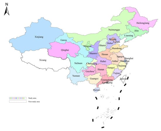
Figure 1.
Scope of the study area.
3. Analysis of Spatial Correlation Network Characteristics of AGTFP in China
3.1. Measurement Results
To clearly demonstrate the temporal evolution characteristics and spatial non-equilibrium state of agricultural green total factor productivity, the kernel density estimation method was used to estimate the probability density function of the variables. We used MATLAB2023b (MathWorks, Natick, MA, USA) software to plot the kernel density distribution of agricultural green total factor productivity in China (Figure 2). The measurement results were analyzed from three aspects: the overall trend, the distribution of the main peak, and the polarization characteristics.
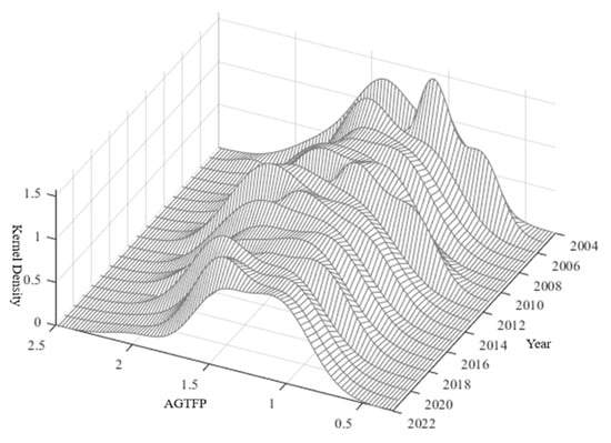
Figure 2.
Kernel density distribution of China’s AGTFP.
From the overall distribution trend of the kernel density function, the distribution center of the kernel density curve for the overall sample was significantly skewed to the right, indicating an overall upward trend in China’s agricultural green total factor productivity. The height of the main peak showed significant fluctuations, suggesting that agricultural green total factor productivity remained at a relatively low level with frequent volatility. From the perspective of the main peak distribution of the kernel density function, the peak value of the main peak during the sample period experienced an alternating evolution of “rise and fall”, with the peak shape gradually transitioning from “sharp and narrow” to “flat and wide”, indicating an expansion in the spatial non-equilibrium of agricultural green total factor productivity across provinces. The overall trend suggests that the differences in agricultural green development levels among provinces are widening. One plausible explanation for this is the significant differences in the division of labor and the status of agricultural green development in the industrial chain among provinces. Additionally, the peak value of the main peak in 2005 was significantly higher, indicating a notable expansion in regional disparities in agricultural green total factor productivity during that period. From the polarization characteristics of the kernel density function, multiple side peaks were evident from 2004 to 2014, while the side peaks were relatively stable from 2015 to 2018. From 2019 to 2022, a single side peak was observed, indicating a clear multi-polarization phenomenon in China’s AGTFP, with distinct polarization characteristics. Furthermore, the sample period showed significant right-tailed characteristics in 2005 and 2022, suggesting spatial spillover effects in interprovincial AGTFP in China.
3.2. Spatial Correlation Network Structure Characteristics
A modified gravity model was employed to transform the “attribute data” of China’s agricultural green total factor productivity (AGTFP) into “relational data”, thereby constructing a spatial connectivity matrix. To visually represent the structural configuration of the spatial network, Gephi 0.10.1 (The Gephi Consortium, Paris, France) software was utilized to generate topological diagrams of the AGTFP spatial connectivity networks for 2004 and 2022 (Figure 3). As revealed in Figure 3, the spatial spillover effects of China’s AGTFP in both 2004 and 2022 exhibited pronounced networked characteristics. These spillover effects transcended geographical proximity between neighboring provinces, establishing connectivity networks across broader geographical spaces.
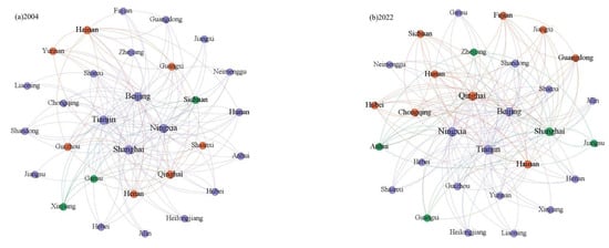
Figure 3.
Topological diagram of the spatial correlation networks in 2004 and 2022.
3.2.1. Overall Network Structural Characteristics
Using Ucinet 6.212 (University of California, Irvine, CA, USA) software, we measured five overall network structural characteristic indicators during the sample observation period (Figure 4). The study found that both the number of network relationships and network density exhibited an evolutionary trend of “increase→decrease→increase→decrease→increase”. Specifically, the number of network relationships rose from 141 in 2004 to 158 in 2022, while network density increased from 0.1621 in 2004 to 0.1816 in 2022. These results indicate that the spatial correlation network maintained robust connectivity and stability, with significant and stable spatial spillover effects observed in interprovincial agricultural green development. Agricultural production inputs—such as labor, technology, and capital—have increasingly transcended geographical proximity constraints, enabling broader cross-regional flows. However, theoretical calculations suggested substantial potential for enhancing interprovincial collaboration in agricultural green development. For instance, the actual number of network relationships peaked at 164 in 2017 (the maximum value within the observation period), yet the theoretical maximum possible relationships between provinces amounted to 870 (30 × 29), revealing a significant gap between actual and theoretical network connectivity.
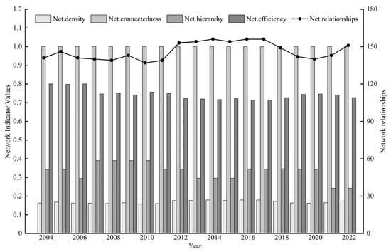
Figure 4.
Overall structural characteristics of the spatial connectivity network, 2004–2022.
As shown in Figure 4, the network connectedness remained at 1 throughout 2004–2022, indicating no unreachable node pairs within the network and reflecting the high accessibility of the spatial correlation network. The network hierarchy measurement results revealed a “V-shaped” decline and rebound from 2004 to 2007 (peaking at 0.3904), followed by a fluctuating downward trend overall, stabilizing at 0.1875 during 2021–2022. This suggests that structural barriers within the network gradually dissolved as the comprehensive abolition of agricultural tax policies was fully implemented, deepening the interactive effects of agricultural green development factors among provinces. Notably, the network hierarchy surged to 0.2941 in 2020, with a growth rate significantly higher than in other years, likely attributable to pandemic control measures triggered by the sudden COVID-19 outbreak [29]. During the observation period, network efficiency decreased from 0.8005 in 2004 to 0.7266 in 2022, implying a reduction in redundant connections within the network and enhanced stability. This reflected lowered transaction costs and optimized spatial allocation in interprovincial flows of agricultural green production factors.
3.2.2. Individual Network Structural Characteristics
Network centrality serves as a critical metric for assessing node importance within a network, providing a systematic framework to quantify the positional influence and functional roles of individual nodes. Using 2022 as a representative case, we conducted a quantitative analysis of three node-level structural characteristic indicators during the study period (Table 4).
Table 4.
Individual structural characteristics of the spatial connectivity network, 2022.
(1) Degree centrality. As shown in Table 3, the mean degree centrality of China’s agricultural green total factor productivity (AGTFP) spatial correlation network in 2022 was 27.126. Provinces with degree centrality values significantly above the mean, ranked in descending order, included Tianjin, Ningxia, Beijing, Qinghai, Shanghai, Hainan, and Fujian. Provinces with values above the mean included Hunan and Chongqing. Higher degree centrality values indicated that these provinces had more network connections, stronger interprovincial linkages, and occupied more central positions in the network, reflecting greater network influence. Furthermore, the measurement results showed that both the out-degree and in-degree means were 5. Thirteen provinces had out-degree values above the mean, ranked in descending order as Fujian, Ningxia, Chongqing, Qinghai, Hainan, Jiangxi, Guangdong, Anhui, Yunnan, Guizhou, Hubei, Hunan, and Tianjin, indicating stronger spatial spillover effects in agricultural green development for these regions. Six provinces had in-degree values above the mean: Tianjin, Ningxia, Beijing, Qinghai, Shanghai, and Hainan, suggesting that agricultural green development factors and resources converged in these provinces, supported by inputs from within the network. Notably, provinces where the in degree significantly exceeded the out degree included Tianjin, Beijing, Shanghai, Ningxia, and Qinghai. These provinces could be categorized into two groups: (1) economically developed regions in the Bohai Rim and eastern coastal areas and (2) economically underdeveloped regions in western China. From the perspective of resource endowments, economically developed regions face constraints in supplying agricultural green production factors, such as land and labor, while western regions lack capital and technological resources. Consequently, both groups exhibited higher dependency on other provinces, leading to the concentration of network resources and factors in these areas.
(2) Closeness centrality. As indicated in Table 3, the mean closeness centrality of China’s AGTFP spatial correlation network in 2022 was 57.038. Provinces with closeness centrality values above the mean, ranked in descending order, included Tianjin, Ningxia, Beijing, Qinghai, Fujian, Shanghai, Hunan, and Chongqing. Higher closeness centrality indicated greater accessibility and information transmission efficiency within the network. In other words, these provinces could more easily establish spatial correlations with others, facilitate information exchange, and promote the flow of agricultural green development factors. Among them, Tianjin exhibited the highest closeness centrality (87.879), positioning it at the center of the local agricultural green total factor productivity (AGTFP) spatial correlation sub-network. This enabled Tianjin to effectively leverage its role in transmitting information and resources, acting as a core actor within the network. Conversely, Hainan had the lowest closeness centrality (47.541), primarily due to geographical constraints that limited its efficiency and capacity to access agricultural green development factors, relegating it to a peripheral actor in the network.
(3) Betweenness centrality. According to the measurements in Table 3, the mean betweenness centrality of China’s agricultural green total factor productivity spatial correlation network in 2022 was 2.808. Provinces with betweenness centrality values above the mean, ranked in descending order, included Tianjin, Ningxia, Qinghai, Beijing, and Shanghai. These provinces acted as strong “intermediaries” within the spatial correlation network, exerting greater control over the regulation of information flows and resource exchanges among other provinces. Notably, Tianjin exhibited the highest betweenness centrality (25.668), solidifying its role as the most critical hub and bridge for factor interactions in the network. Provinces with relatively low betweenness centrality rankings, such as Hebei, Liaoning, Jiangsu, Xinjiang, and Gansu, were predominantly located in geographically remote areas (except Jiangsu), rendering them more susceptible to control and dominance by other provinces in terms of agricultural green development factors and resources. It is worth emphasizing that the combined betweenness centrality of the top five provinces (Tianjin, Ningxia, Qinghai, Beijing, and Shanghai) totaled 71.159, accounting for over 84% of the total betweenness centrality across all 30 provinces. In contrast, the combined value of the bottom five provinces constituted only approximately 0.32% of the total, highlighting a pronounced imbalance in the distribution of betweenness centrality among provinces.
3.2.3. Spatial Clustering Analysis
Using the CONCOR method in social network analysis, with a maximum depth of splits set to 2 and convergence criteria of 0.2, the 30 provinces in China were divided into 4 sections to characterize and analyze the spatial clustering features of the agricultural green total factor productivity spatial correlation network. The classification results are presented in Table 5. Based on the earlier calculations, the agricultural green total factor productivity spatial correlation network in 2022 comprised 158 total connections, including 17 intra-section ties and 141 inter-section ties, indicating significant spatial correlations and spillover effects among the sections. Specifically:
Table 5.
Section types of the AGTFP spatial correlation network.
Section I included 16 provinces: Heilongjiang, Jilin, Anhui, Hubei, Hunan, Jiangxi, Sichuan, Guangxi, Guizhou, Xinjiang, Yunnan, Fujian, Jiangsu, Chongqing, Zhejiang, and Guangdong. Most of these provinces are either major grain-producing regions or economically developed coastal areas in eastern China.
Section II consisted of 8 provinces: Henan, Shanxi, Shandong, Hebei, Shaanxi, Gansu, Liaoning, and Inner Mongolia, predominantly located in central and western China.
Section III comprised 4 members: Beijing, Shanghai, Tianjin, and Ningxia. Except for Ningxia (a western remote region), all are highly urbanized municipalities.
Section IV included 2 provinces: Qinghai and Hainan.
As shown in Table 5, Section I had 64 spillover ties and 22 receiving ties, with spillover ties significantly exceeding receiving ties. Most members of this section are located in China’s major grain-producing regions and economically developed coastal areas in eastern China, possessing abundant agricultural green development resources. Their substantial spillover effects on factor resources to other sections classify this group as a net-spillover section.
Section II exhibited 28 spillover ties and 24 receiving ties, with both values relatively high. Its members are predominantly in central and western regions, acting as a hub for the exchange and flow of agricultural production factors (e.g., technology, capital, and labor) between eastern and western China, thus categorized as a broker section.
Section III had 32 spillover ties and 57 receiving ties, with receiving ties far surpassing spillover ties. Its members are primarily highly urbanized municipalities (excluding Ningxia), which face relatively limited agricultural green production resources and factors. As the primary beneficiaries of the network, this group is classified as a net-beneficiary section.
Section IV included 17 spillover ties and 38 receiving ties. Its members possess moderate agricultural green development scales and distinct policy advantages, enabling them to both receive spillovers from other sections and generate spillover effects, thus categorized as a bidirectional spillover section.
Notably, the actual intra-section ratios across the network were significantly lower than the expected intra-section ratios, indicating untapped potential for intra-section spatial spillovers.
Furthermore, drawing on the research of Huajun Liu [41], we calculated the network density matrices for the four sections. Based on earlier measurements, the overall network density of China’s AGTFP spatial correlation network in 2022 was 0.1816. Sections with a network density greater than the overall value were assigned a value of 1, while those below it were assigned 0. Using this criterion, the section density matrices were converted into image matrices to examine spatial correlation relationships and spillover pathways among the four sections. The results of the section density matrices and image matrices are presented in Table 6. Additionally, based on the measurements from Table 5 and Table 6, a spatial correlation diagram (Figure 5) was constructed to visualize the inter-section relationships and transmission mechanisms.
Table 6.
Inter-section spillover effects of the AGTFP spatial correlation network.
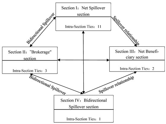
Figure 5.
Spatial inter-section correlation relationships among the four sections of AGTFP in China.
As shown in Table 5 and Figure 5, significant intra-section correlations existed within Section I, which exhibited bidirectional spillover effects with Section II and influenced the agricultural green development of Sections III and IV through spillover effects. This indicates that provinces within Section I possessed robust agricultural production factor inputs and advanced green production technologies, enabling them to meet their own development needs while exporting factors and technologies to other regions. Section II generated spillover effects on Section I and maintained bidirectional spillover relationships with Sections III and IV, highlighting its role as an intermediary in the spatial correlation network. The advantageous geographical conditions of its member provinces facilitated rapid aggregation and dispersion of agricultural green development factors and resources. Section III exerted spillover effects on Section II, reflecting its comparative advantages in the AGTFP spatial correlation network. Section IV generated spillover effects on Sections I–III.
Looking at it from a general point of view, agricultural green production factors from China’s major grain-producing regions and economically developed coastal areas in the east are transferred to other provinces via spillover effects. The central and western regions act as critical intermediaries in the transmission of factors and resources. Meanwhile, highly urbanized municipalities and western regions emerge as net beneficiaries of the AGTFP spatial correlation network, securing substantial relational gains within the overall network [42].
4. Driving Mechanisms of the Spatial Correlation Network of AGTFP in China
Analysis of Regression Results Based on the QAP Method
Following Equation (6), we conducted QAP regressions with 5000 random permutations for representative years (2004, 2008, 2012, 2016, and 2020) at 4-year intervals. As reported in Table 6, all coefficients demonstrated statistical significance at the 1% level (p < 0.01), with adjusted values ranging from 0.113 to 0.258. Additionally, Table 7 presents regression results for difference matrices constructed using the absolute differences in average values of corresponding indicators across provinces from 2004 to 2022.
Table 7.
QAP regression results of driving factors in the spatial correlation network of AGTFP.
Overall, the formation and evolution of the spatial correlation network of agricultural green total factor productivity (AGTFP) in China resulted from the differential directions and intensities of internal and external driving factors. Specifically:
(1) Geographical proximity. The regression coefficient of geographical proximity remained significantly positive throughout the sample period, revealing that geographical distance between provinces played a critical role in shaping spatial correlations.
(2) Differences in fiscal support. The regression coefficient of fiscal support disparities was consistently significantly positive, indicating that differences in government financial support for agriculture were positively correlated with spatial spillover effects of agricultural green development. A plausible explanation is that narrowing fiscal support gaps enhanced resource acquisition capabilities for provinces with poor agricultural green development endowments, thereby generating stronger spatial spillovers.
(3) Differences in green technology progress index. The regression coefficient of green technology progress index disparities was significantly positive, suggesting that widening gaps in agricultural green technology levels between provinces foster technology spillovers by incentivizing interprovincial exchanges and cooperation. This phenomenon arises because large disparities create a “technology gap”, where differences in technological endowments drive cross-regional collaboration to bridge such gaps.
(4) Differences in rural labor force size. The regression coefficient of rural labor force scale disparities was significantly positive, demonstrating a positive but fluctuating impact on spatial spillover effects. The driving mechanism lies in cross-regional labor mobility, which introduces advanced cultivation techniques and standardized production practices, thereby enhancing specialization and fostering closer green agricultural collaboration.
(5) Differences in agricultural industrial structure. The regression coefficient transitioned from positive to negative over the sample period, with a negative mean coefficient. This implies that emerging agricultural service sectors (e.g., rural tourism) mitigate disparities caused by monoculture-dominated structures, ultimately strengthening spatial network linkages.
(6) Differences in agricultural economic development levels. The regression coefficient alternated between positive and negative values during the sample period, though the mean coefficient was significantly positive. The directional variability may relate to natural condition fluctuations in regional agricultural production. Overall, however, disparities in agricultural economic development levels positively influenced spatial spillover effects. A potential explanation is that such disparities create a “potential gradient”, serving as a primary driving force for cross-regional flows of production factors and resources.
5. Conclusions and Policy Implications
5.1. Conclusions
This study investigated the spatial correlation network and driving mechanisms of China’s agricultural green development through the lens of agricultural green total factor productivity (AGTFP), providing empirical evidence for the existence of spatial spillover effects in this domain. The key findings were as follow:
(1) Network connectedness measures were all equal 1, indicating the absence of unreachable node pairs within the overall network. Both network hierarchy and network efficiency exhibited a fluctuating downward trend, reflecting the gradual dismantling of structural barriers and a reduction in redundant connections. The interprovincial agricultural green development spatial association network in China demonstrated strong connectivity, stability, and accessibility.
(2) The quantity and spatial concentration of agricultural green development associations steadily increased, with a few dominant provinces becoming hubs for the aggregation, regulation, and allocation of green development resources. Major grain-producing regions and economically developed eastern coastal areas acted as key drivers of spatial spillover effects, while central and western regions played a “broker” role in absorbing and transferring resources within the network. Municipalities such as Tianjin and Shanghai exhibited siphon effects, drawing resources from other provinces.
(3) Driving factors exhibited distinct heterogeneity and volatility in their directional impacts and intensity on the AGTFP spatial association network. Strengthening government financial support, enhancing rural labor talent reserves, improving green technology advancement efficiency, and elevating agricultural economic development levels are critical for fostering spatial associations and unlocking the spillover potential of agricultural green development. Interprovincial disparities in China’s agricultural industrial structure inhibited the formation of spatial association networks.
5.2. Policy Implications
First, top-level design should be strengthened to jointly formulate and implement green agriculture standards, promoting policy coordination and resource information sharing for agricultural green development. Market-oriented reforms can be deepened in the agricultural sector, accelerating the construction of a unified national market, breaking down regional blockades (e.g., fragmented organic certification standards, interprovincial market access restrictions for green products, and localized use of ecological compensation funds), further reducing the cross-regional flow costs of production factors, such as technology, capital, and labor, enhancing the reciprocal linkage effects of agricultural green development, promoting optimal allocation of agricultural resources, and achieving coordinated green development of agriculture across regions.
Second, precise and targeted policy measures should be introduced according to local conditions. It is important to strengthen the leading role of “core” provinces, such as Tianjin, improve the system of technological innovation and agricultural technology extension, jointly promote the research, development, and dissemination of green agricultural technologies, fully leverage the technology spillover effects, lead industrial upgrading through technological innovation, and drive regional agricultural green development. Policymakers should enhance the resource regulation capacity of “broker” provinces, such as Henan, accelerate the construction of interconnected infrastructure in the agricultural sector, reduce barriers to the flow of resource elements between regions, build cooperation and exchange bridges, such as information platforms for agricultural green development, create strategic pivots for the cross-regional flow of green agricultural elements, and improve the efficiency and precision of resource regulation. Further, they should promote balanced development in “peripheral” provinces in the west by increasing policy support, establishing guarantee and assistance mechanisms, enhancing the capacity to undertake industrial funds, technology, and other resources, exploring practical paths for cross-regional dislocation development, reducing regional disparities and imbalances, and achieving comprehensive improvement in agricultural green development.
Third, we should fully utilize geographical advantages and resource endowment conditions, explore differentiated development pathways, strengthen exchanges and cooperation in agricultural green development with neighboring provinces, and avoid homogeneous competition. It is important to increase financial support and investment in agricultural green technology research and development and improve the dissemination of advanced agricultural green production technologies through training and demonstration. Policymakers should enhance the scale and intensification level of agricultural production and accelerate the pace of agricultural modernization. They should also optimize the agricultural industrial structure and reduce the inhibitory effect of agricultural industrial structure differences on the spatial correlation network. At the same time, they must pay attention to the phased characteristics of policy implementation, timely optimize and adjust strategies, maximize the comprehensive effects of policies, and promote new breakthroughs in China’s agricultural green transformation and high-quality development.
Future research could extend this work by exploring dynamic evolution mechanisms of spatial spillover networks in agricultural green development across finer geographical scales (e.g., prefecture-level cities or counties) to address intra-provincial heterogeneity. Integrating multi-dimensional indicators, such as digital agricultural technologies or carbon-trading policies, into the analysis framework may further clarify how emerging factors reshape spatial linkages. Additionally, conducting scenario simulations to assess the impact of differentiated regional policies (e.g., fiscal incentives for green technologies or cross-regional ecological compensation mechanisms) on network structures would provide actionable insights for optimizing resource allocation.
Author Contributions
Conceptualization, Y.H.; methodology, Y.H. and G.F.; software, Y.H.; validation, G.F.; formal analysis, G.F. and Y.G.; resources, Y.H.; data curation, Y.H. and G.F.; writing—original draft preparation, Y.H.; writing—review and editing, Y.H., C.Q., and Y.G.; visualization, Y.H. and Y.G.; supervision, C.Q.; project administration, C.Q.; funding acquisition, C.Q. All authors have read and agreed to the published version of the manuscript.
Funding
This research was funded by the China Agriculture Research System—National Citrus Industry Technology System (CARS-26-06BY), the National Social Science Fund of China (23BJY155), and the Strategic Research and Consulting Project of the Chinese Academy of Engineering “Innovative Development Strategy of Characteristic Fruit Industry in Hunan Province” (2024WK1003).
Institutional Review Board Statement
Not applicable.
Data Availability Statement
The data presented in this study are available from the first author upon request.
Conflicts of Interest
The authors declare no conflicts of interest.
References
- Zhou, Y.S.; Yin, Z.J. Does agricultural insurance promote agricultural green development in China? J. Huazhong Agric. Univ. Soc. Sci. Ed. 2024, 01, 49–61. (In Chinese) [Google Scholar]
- Wang, X.; Yang, C.; Qiao, C. Agricultural Service Trade and Green Development: A Perspective Based on China’s Agricultural Total Factor Productivity. Sustainability 2024, 16, 7963. [Google Scholar] [CrossRef]
- Liu, Y.W.; Ouyang, Y.; Cai, H.Y. Measurement and spatio-temporal evolution characteristics of agricultural green total factor productivity in China. J. Quant. Tech. Econ. 2021, 38, 39–56. (In Chinese) [Google Scholar]
- Huang, X.Q.; Feng, C.; Qin, J.H.; Wang, X.; Zhang, T. Measuring China’s agricultural green total factor productivity and its drivers during 1998–2019. Sci. Total Environ. 2022, 829, 154477. [Google Scholar] [CrossRef]
- Hamid, S.; Wang, Q.; Wang, K. The spatiotemporal dynamic evolution and influencing factors of agricultural green total factor productivity in Southeast Asia (ASEAN-6). Environ. Dev. Sustain. 2025, 27, 2469–2493. [Google Scholar] [CrossRef]
- Fang, L.; Hu, R.; Mao, H.; Chen, S.J. How crop insurance influences agricultural green total factor productivity: Evidence from Chinese farmers. J. Clean. Prod. 2021, 321, 128977. [Google Scholar]
- Song, M.L.; Du, J.T.; Tan, K.H. Impact of fiscal decentralization on green total factor productivity. Int. J. Prod. Econ. 2018, 205, 359–367. [Google Scholar]
- Chen, Y.F.; Miao, J.F.; Zhu, Z.T. Measuring green total factor productivity of China’s agricultural sector: A three-stage SBM-DEA model with non-point source pollution and CO2 emissions. J. Clean. Prod. 2021, 318, 128543. [Google Scholar]
- Tone, K. A slacks-based measure of efficiency in data envelopment analysis. Eur. J. Oper. Res. 2001, 130, 498–509. [Google Scholar] [CrossRef]
- Guo, H.H.; Liu, X.M. Spatio-temporal evolution of agricultural green total factor productivity in China. Chin. J. Manag. Sci. 2020, 28, 66–75. (In Chinese) [Google Scholar]
- Liu, Z.; Dai, X. Analysis on the Growth and Convergence of Agricultural Green Total Factor Productivity in Guangxi. Front. Humanit. Soc. Sci. 2023, 3, 94–102. [Google Scholar]
- Xiao, Q.; Zhou, Z.Y.; Luo, Q.Y. Agricultural green production efficiency and its spatio-temporal differentiation in the Yangtze River Economic Belt. Chin. J. Agric. Resour. Reg. Plan. 2020, 41, 15–24. (In Chinese) [Google Scholar]
- Wang, F.; Wang, H.; Liu, C. Does economic agglomeration improve agricultural green total factor productivity? Evidence from China’s Yangtze river delta. Sci. Prog. 2022, 105, 460. [Google Scholar]
- Yang, Q.; Wang, J.; Li, C.; Liu, X.P. Spatial differentiation and driving factors of agricultural green total factor productivity in China. J. Quant. Tech. Econ. 2019, 36, 21–37. (In Chinese) [Google Scholar]
- Wang, S.; Zhu, J.; Wang, L. The inhibitory effect of agricultural fiscal expenditure on agricultural green total factor productivity. Sci. Rep. 2022, 12, 20933. [Google Scholar]
- Gu, Y.; Qi, C.; He, Y.; Liu, F.; Luo, B. Spatial Correlation Network Structure of and Factors Influencing Technological Progress in Citrus-Producing Regions in China. Agriculture 2023, 13, 2118. [Google Scholar] [CrossRef]
- Yang, W.P.; Zhang, Q. Impact of biased technological progress on agricultural total factor productivity growth in China. J. Bus. Econ. 2024, 52–66. (In Chinese) [Google Scholar]
- Xu, L.; Jiang, J.; Du, J. The Dual Effects of Environmental Regulation and Financial Support for Agriculture on Agricultural Green Development: Spatial Spillover Effects and Spatio-Temporal Heterogeneity. Appl. Sci. 2022, 12, 11609. [Google Scholar] [CrossRef]
- Shi, C.L. Impact of land transfer on agricultural high-quality development: A perspective of green total factor productivity. J. Nat. Resour. 2024, 39, 1418–1433. (In Chinese) [Google Scholar]
- Zhan, Y.Q.; Wang, W.; Ren, Y.H. Inspection supervision and corporate green total factor productivity. Financ. Res. Lett. 2024, 67, 105805. [Google Scholar]
- Zhang, C.Y.; Zhu, H.; Li, X.Z. Which productivity can promote clean energy transition-total factor productivity or green total factor productivity? J. Environ. Manag. 2024, 366, 121899. [Google Scholar] [CrossRef]
- Xiao, B.Y.; Li, H.B. Financial efficiency, green innovation and green total factor productivity. Financ. Res. Lett. 2025, 76, 107005. [Google Scholar] [CrossRef]
- Du, J.; Wang, R.; Wang, X.H. Environmental total factor productivity and agricultural growth: A two-stage analysis based on DEA-GML index and panel Tobit model. Chin. Rural. Econ. 2016, 65–81. (In Chinese) [Google Scholar] [CrossRef]
- Gelb, J.; Apparicio, P. Temporal Network Kernel Density Estimation. Geogr. Anal. 2024, 56, 62–78. [Google Scholar] [CrossRef]
- Zhao, L.; Cao, N.G.; Han, Z.L.; Gao, X.T. Evolution Characteristics and Influencing Factors of the Spatial Correlation Network of Green Economic Efficiency in China. Resour. Sci. 2021, 43, 1933–1946. (In Chinese) [Google Scholar]
- Ge, P.F.; Wang, S.J.; Huang, X.L. Measurement of China’s agricultural green total factor productivity. China Popul. Resour. Environ. 2018, 28, 66–74. (In Chinese) [Google Scholar]
- Song, Y.P.; Fan, X.Q.; Geng, P.P. Scale operation and agricultural green development: Observations based on agricultural green total factor productivity. J. Huazhong Agric. Univ. Soc. Sci. Ed. 2024, 57–70. (In Chinese) [Google Scholar] [CrossRef]
- Zhu, H.G.; Cao, B.; Zhao, W.C. Temporal evolution and spatial convergence characteristics of agricultural total factor carbon emission performance in China. Stat. Decis. 2022, 38, 63–68. (In Chinese) [Google Scholar]
- Qian, Z.Y.; Liu, S.J. Spatial Correlation Network Structure Characteristics and Driving Factors Identification of Agricultural Green Low-Carbon Production Efficiency in the Yellow River Basin. J. Arid Land Resour. Environ. 2024, 38, 27–38. (In Chinese) [Google Scholar]
- Yang, X.; Li, D.T.; Cao, J.M. Spatial Correlation Analysis of Beef Cattle Production in Southern China and Industrial Development Pathways. Chin. J. Agric. Resour. Reg. Plan. 2023, 44, 214–223. (In Chinese) [Google Scholar]
- Wang, F.; Wu, L.; Zhang, F. Network Structure and Influencing Factors of Agricultural Science and Technology Innovation Spatial Correlation Network—A Study Based on Data from 30 Provinces in China. Symmetry 2020, 12, 1773. [Google Scholar] [CrossRef]
- Matias, R.; Paloma, B.; Ian, C.; Ivan, H. The role of social networks in the inclusion of small-scale producers in agri-food developing clusters. Food Policy 2018, 77, 59–70. [Google Scholar]
- He, W.; Wang, F.; Feng, N. Research on the characteristics and influencing factors of the spatial correlation network of cultivated land utilization ecological efficiency in the upper reaches of the Yangtze River, China. PLoS ONE 2024, 19, e0297933. [Google Scholar]
- Liu, P.; Qin, Y.; Luo, Y.Y.; Wang, X.X.; Guo, X.W. Structure of low-carbon economy spatial correlation network in urban agglomeration. J. Clean. Prod. 2023, 394, 136359. [Google Scholar]
- He, Y.; Li, Z.F.; Fang, G.Z.; Qi, C.J. Spatial Correlation Effects of Citrus Prices in Major Production Areas: Based on VAR Model and Social Network Analysis Method. Chin. J. Agric. Resour. Reg. Plan. 2023, 44, 174–183. (In Chinese) [Google Scholar]
- Han, X.Y.; Zhang, X.; Lei, H. Analysis of the spatial association network structure of water-intensive utilization efficiency and its driving factors in the Yellow River Basin. Ecol. Indic. 2024, 158, 111400. [Google Scholar]
- Bai, R.; Lin, B.Q. An in-depth analysis of green innovation efficiency: New evidence based on club convergence and spatial correlation network. Energy Econ. 2024, 132, 107424. [Google Scholar] [CrossRef]
- Liu, S.; Yuan, J. Spatial correlation network structure of energy-environment efficiency and its driving factors: A case study of the Yangtze River Delta Urban Agglomeration. Sci. Rep. 2023, 13, 20790. [Google Scholar]
- Fang, H.; Chai, J.; Wang, Z.; Zhang, R.; Huang, C.; Luo, M. Exploring the Spatial Correlation Network and Its Formation Mechanisms in Urban Land Use Performance: A Case Study of the Yangtze River Economic Belt. Land 2024, 13, 1019. [Google Scholar] [CrossRef]
- Wang, Z.S.; Xie, W.C.; Zhang, C.Y. Towards COP26 targets: Characteristics and influencing factors of spatial correlation network structure on U.S. carbon emission. Resour. Policy 2023, 81, 103285. [Google Scholar]
- Liu, H.J.; Liu, C.M.; Sun, Y.N. Spatial correlation network structure characteristics and effects of energy consumption in China. China Ind. Econ. 2015, 83–95. (In Chinese) [Google Scholar] [CrossRef]
- Tan, R.H.; Liu, H.M. Spatial Correlation Network Characteristics Evolution and Influencing Factors of Agricultural Green Total Factor Productivity in China. Chin. J. Eco-Agric. 2022, 30, 2011–2026. (In Chinese) [Google Scholar]
Disclaimer/Publisher’s Note: The statements, opinions and data contained in all publications are solely those of the individual author(s) and contributor(s) and not of MDPI and/or the editor(s). MDPI and/or the editor(s) disclaim responsibility for any injury to people or property resulting from any ideas, methods, instructions or products referred to in the content. |
© 2025 by the authors. Licensee MDPI, Basel, Switzerland. This article is an open access article distributed under the terms and conditions of the Creative Commons Attribution (CC BY) license (https://creativecommons.org/licenses/by/4.0/).