Robust Guidance and Selective Spraying Based on Deep Learning for an Advanced Four-Wheeled Farming Robot

Abstract

Complex farmland backgrounds and varying light intensities make the detection of guidance paths more difficult, even with computer vision technology. In this study, a robust line extraction approach for use in vision-guided farming robot navigation is proposed. The crops, drip irrigation belts, and ridges are extracted through a deep learning method to form multiple navigation feature points, which are then fitted into a regression line using the least squares method. Furthermore, deep learning-driven methods are used to detect weeds and unhealthy crops. Programmed proportional–integral–derivative (PID) speed control and fuzzy logic-based steering control are embedded in a low-cost hardware system and assist a highly maneuverable farming robot in maintaining forward movement at a constant speed and performing selective spraying operations efficiently. The experimental results show that under different weather conditions, the farming robot can maintain a deviation angle of 1 degree at a speed of 12.5 cm/s and perform selective spraying operations efficiently. The effective weed coverage (EWC) and ineffective weed coverage (IWC) reached 83% and 8%, respectively, and the pesticide reduction reached 53%. Detailed analysis and evaluation of the proposed scheme are also illustrated in this paper.

1. Introduction

In the rapid development of smart technologies, their integration into agriculture has been critical to combating labor scarcity and an aging workforce. Contemporary practices in crop management, including plant monitoring, watering, pesticide spraying, and fertilizing, are still often performed manually using machines and tools. This requires farmers to focus on field operations for a long time, which results in long working hours and high labor costs. The proven efficacy of automation in performing monotonous tasks has seen its adoption across various sectors, with its applicability in agriculture being equally comprehensive, encompassing activities like weeding and harvesting [1]. Traditional small-scale agricultural robots were designed to navigate based on sensor fusion methods, which are suitable for structured environments [2]. Relying on the improvement of precision agriculture technology, the real-time kinemetric (RTK) global navigation satellite system (GNSS) (RTK-GNSS) and machine vision have played an important role in automatic guidance technology. RTK-GNSS has been pivotal in providing precise metrics for positioning, velocity, and timing, which assists users in planning the robot’s movement path [3,4]. In particular, after the user can define multiple specific positions to form a path in a known field environment, the robot can then autonomously move to that point to perform field operations and reduce errors through heading control [5,6].

With the improvement of computer computing performance, machine vision technology has been used to identify, track, and measure targets and perform image processing [7]. Its technology has low development costs, is easy to maintain, and has wide applicability [8,9,10,11,12,13,14]. Morphology-based methods have been used to extract guide lines from rice field images, enabling autonomous weeding robots to operate without damaging crops [9,10]. This approach initially involved grayscale or CIE-Lab color space images, followed by Otsu thresholding and thinning processes to extract the edges of plant objects. The traditional crop row detection method often fails due to the influence of excessive ambient light or crop occlusion and other issues. Therefore, the method of using soil distribution information to find guidance points has been proven to be able to correctly find crop lines [11]. Post-identification Hough transform operations are utilized for edge detection, and the median lines between them serve as navigation lines, guiding unmanned vehicles through field operations autonomously [12]. The method of obtaining path fitting from grayscale images of specific areas of interest through image segmentation, navigation point extraction, and predicted point Hough transforms has been proven to be effective to improve the computational efficiency of the traditional Hough transform [13]. Meanwhile, this method can also solve the problem of insufficient accuracy caused by using the least squares method.

Based on the above description, the Hough transform and least squares method were the most commonly used path fitting methods in crop row identification. Among them, Hough processing easily extracts feature edge lines and then obtains the crop lines. The least squares rule is a statistical method of regression analysis which can fit a navigation path with acceptable accuracy. Although both methods can detect row guide lines, different environmental conditions, such as variations in color, brightness, saturation, contrast, reflection, shadow, occlusion, and noise in the same scene, can lead to the failure of guidance line extraction [15,16]. Secondly, differences in wind intensity in the field will also cause plant movement, which will blur the plant image and cause inaccurate crop center point detection [17,18,19].

With the advancements in high-speed computing technology, employing deep learning for navigation line extraction has gained traction. A U-Net deep learning model has been used to detect crops without interruption in the field, given favorable weather conditions, suitable lighting, few weeds, and neatly arranged crops. Finally, the Hough transform operation was used to identify the guidance lines [20]. The crop row extraction method based on Tiny-YOLOv4 can quickly detect multiple objects in an image and extract crop feature points within the frame through binarization operations and mean filtering operations. Finally, regression analysis with the least squares method was used to fit a guidance line [21]. An object detection method combining YOLO-R and density-based spatial clustering of applications with noise (DBSCAN) can quickly identify the number of crop rows and the crops in each row. Crop row lines can be found through the least squares method, and under different rice growth stages, the crop row recognition rate reaches at least 89.87% [22].

Deep learning methods have also been frequently employed in robotics for the identification of weeds and crops. Various research endeavors highlight the effectiveness of these advanced techniques in precision agriculture. Among them, the YOLO-based method has been commonly used to detect weeds in the field [23,24,25,26,27,28]. Ruigrok et al. [23] used the trained YOLO v3 model to detect weeds and spray them. The results showed that 96% of the weeds were controlled, but about 3% of the crops were sprayed by mistake. Twelve types of weeds in rice fields were detected by the trained YOLO v4 model, with an accuracy of 97% and an average detection time of 377 ms [24]. A weeding robot with deep learning developed by Chang et al. [25] could remove weeds at a speed of 15 cm per second, with an efficiency rating of 88.6%. The trained YOLO v5 model was utilized for weed (Solanum rostratum Dunal) detection, and the accuracy and recall rate of the model were 95% and 90%, respectively [26]. The YOLO-sesame model was used to identify weeds and crops in sesame fields, and its results showed a mean accuracy (mAP) of 96.1% at a frame rate of 36.8 frames per second (FPS) [27]. Utilizing the YOLO v3 model for weed detection, as detailed by Ruigrok et al., they trained it on image data from 20 different fields and tested it in 5 different arable fields [28]. The results indicated that increasing the variance in training data while keeping the sample size constant could reduce the generalization error during detection. Five deep learning models were used to detect weeds in soybean fields, with a custom five-layer CNN architecture showing a high detection accuracy of 97.7% and the lowest latency and memory usage [29].

With the four-wheel steering mechanism and flexible steering control method, the robot can move on any terrain on the site with high maneuverability and avoid slipping. Common steering control methods are based on Ackerman steering principle technology [30,31] combined with proportional–integral–derivative (PID), fuzzy logic, and sliding mode control [5,6,12,32].

The purpose of efficient guidance and control systems for agricultural robots is to accurately perform tasks such as spraying and weeding. However, a large part of existing research is still limited to the field of offline simulation or laboratory experiments, or they were only used to demonstrate crop row guidance performance, with little empirical evidence to support their applicability in real-world agricultural task operations.

In the real field, the surface appearance of field soil is constantly changing in farmland. During fallow periods, farmland may exhibit only furrows or what are referred to as drip irrigation belts interspersed between ridges. In contrast, the planting season may present a mix of crops and ridges without the consistent presence of irrigation belts or, in some instances, exclusively crops, contingent upon individual agricultural practices. Many studies often focus on feature extraction of single objects in the field. Once the features of objects in the field are unclear or do not exist, the method used often loses the guidance line, especially in low-light environments. Compounding these challenges is the reliance on a singular type of object for training datasets, thereby critically hampering the universality and adaptability of the detection models. Aside from that, open field images are often used for crop line detection. In practice, these images are often exposed, causing the detection model to be unable to identify crop row lines. It is uncertain whether these methods can be used for detection during robot motion or achieve the same detection performance. Furthermore, field testing and validation of these integrated approaches for steering control and task execution remains challenging.

In this study, the proposed scheme was used to automatically detect potential guidance lines on field ridges with deep learning and least squares regression, using a PID controller and fuzzy logic controller (FLC) to maintain the travel speed and heading angle. By adopting the one-stage object detection framework, the robot operation system was tailored for various object recognition tasks such as crop identification, drip irrigation belt detection, ridge recognition, weed detection, and identification of crops with nutrient deficiencies. It was also specifically designed to analyze and compare the object detection performance of the trained models at different FPS and obtain the real-time processing performance of the detection model in a field under different weather conditions. In terms of field operations, the smart sprayers were designed to spray nutrient-deficient crops as well as weeds.

The organization of this paper is as follows. Section 2 introduces the methodology, including the motion model of a farming robot, guidance line generation, methods for controlling the speed and heading of the robot, and spraying operation. Section 3 describes the configuration of each module within the robot.Section 4 discusses the experimental results, including tests of autonomous guidance of the robot, identification of weeds and unhealthy crops, and tests of selective spraying system performance. Finally, Section 5 provides the conclusions, summarizing the main findings of this study.

2. Autonomous Navigation and Selective Spraying Scheme

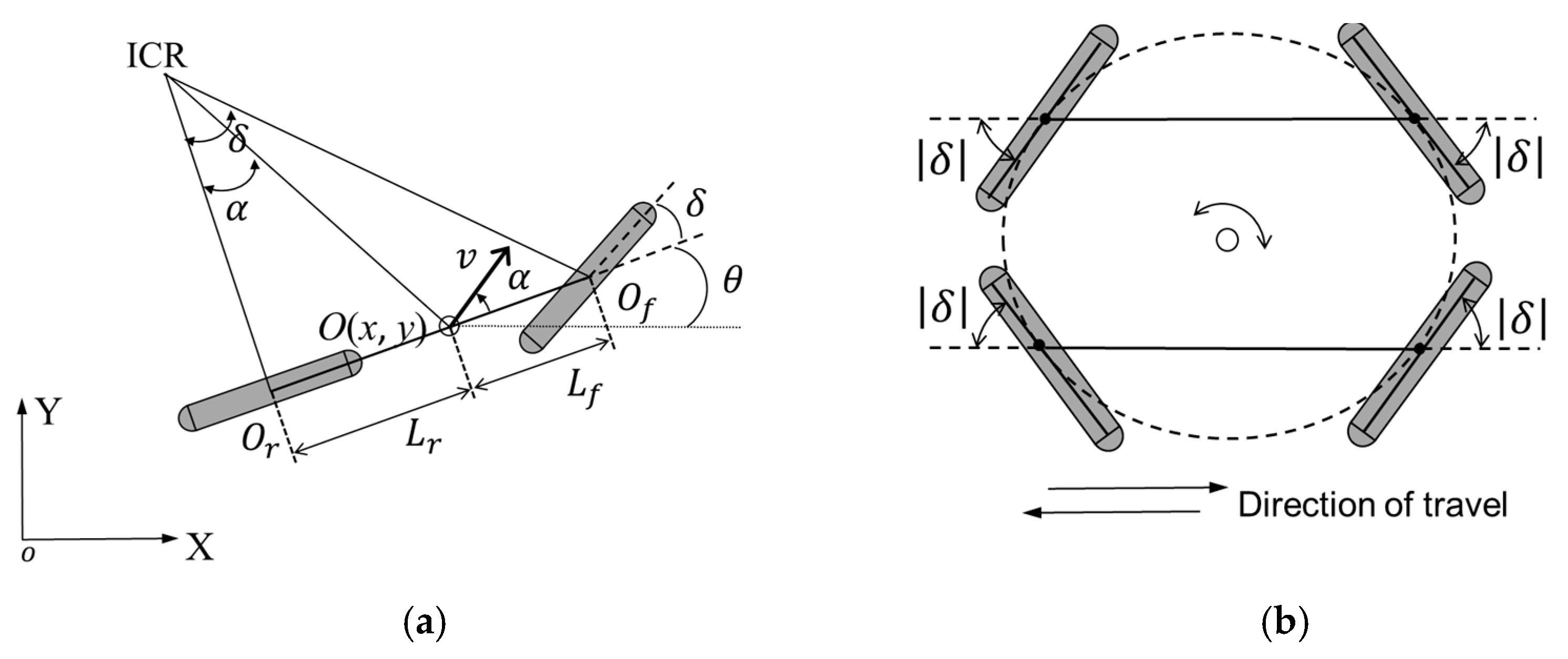
2.1. Motion Model

Given the constant and relatively slow travel speed of the robot, along with its rigid tires, its motion state at any given moment can be described using a bicycle model [33] as shown in Figure 1a. The global X-Y coordinate plane is a fixed horizontal plane upon which the robot moves and is used to describe its motion. It was assumed that $O$, $O_f$, and $O_r$ represent the center of gravity of the robot, the center of the rear wheel, and the center of the front wheel, respectively. The distance between the center of the front wheel and the robot’s center of gravity is denoted as $L_f$, while $L_r$ is the distance between the center of the rear wheel and the center of gravity of the robot. The slip angle was represented by α, the heading angle by θ, and the speed at the center of gravity by ν, with its component velocities being $\dot{x}$ and $\dot{y}$. This motion model is based on front-wheel steering, assuming the direction of the rear wheels is parallel to the robot body. The kinematic model of the robot is represented by ($\dot{x}$, $\dot{y}$, $\dot{\theta }$):

$$\dot{x}=v\cos (\theta +\alpha )$$

(1)

$$\dot{y}=v\sin (\theta +\alpha )$$

(2)

$$\dot{\theta }=\frac{v\cos \alpha \tan \delta }{L_f+L_r}$$

(3)

Figure 1. The motion mode of the robot. (a) A bicycle model for straight-line movement of the robot. (b) The steering angle of the four wheels in spin-on-the-spot mode. $\left|·\right|$ stands for an absolute value operation.

The velocity $v$ is given by $v=\frac{v_f\cos \delta {+v}_r}{2\cos \alpha }$, where $v_f$ and $v_r$ represent the velocities of the front and rear wheel, respectively. The slip angle $\alpha$ is calculated as $\alpha ={\tan }^{-1}\left(\frac{L_r\tan \delta }{L_f+L_r}\right)$. When the robot moves in a straight line, the steering angle δ of both of the front wheels is within the range from −δ_max to +δ_max, and the steering angle of both the rear wheels is fixed at zero. Moreover, during turning maneuvers, all wheels assumed the same steering angle $\left|\delta \right|$, putting the robot in a state of on-the-spot rotation (Figure 1b).

2.2. Guidance Line Generation

First, the top in-view image of the field is captured by a digital camera. The target objects in the image consist of ridges, crops, or a drip irrigation belt (Figure 2a). In order to form a guidance line, the original image is divided into two sub-images through a masking operation, which covers the long strip area in the center of the image with a white color (see Figure 2b). Subsequently, deep learning techniques are utilized to detect the ridges, crops, or drip irrigation belt within the image, as shown in Figure 2c. Meanwhile, the center point of each object is also extracted.

Figure 2. An xample of object detection in the image of the ridge. (a) The original image. (b) The original image divided into two sub-images through masking processing. (c) An example of object detection results. Red dot = center point of object; green box = detected objects (ridges, crops, or drip irrigation belt).

The tool used for labeling the ridges, crops, and drip irrigation belt in the image was LabelImg, which executes the LabelImg script through Anaconda. This tool marks the positions of objects in each image and generates an XML file containing information about the objects and their positions, providing training data for the dataset. In this study, YOLO v4 was used as the object detector [34], and its architecture is based on YOLO v3, which was proposed by Joseph Redmon [35]. YOLO v4 is proficient at identifying small objects at high speeds while maintaining a certain level of recognition accuracy. The architecture of YOLO v4 includes three core parts: the backbone, the neck, and the detection head. As shown in Figure 3, CSPDarknet53 serves as the backbone network for the object detector. Its structure is based on DenseNet, which functions to connect layers in a convolutional neural network and adds a cross-stage partial network (CSPNet) [36]. Splitting and merging techniques are used to obtain a more efficient flow of gradient information and improve the accuracy of gradient calculations. The deep features of the image are then introduced into the neck layer, which separates the smallest-scale features from the backbone and pools multiple sizes to increase the receptive field.

Figure 3. The framework of YOLO v4.

The Path Aggregation Network (PANet) uses feature maps formulated through spatial pyramid pooling (SPP) [37] and CSP-Darknet53 at each level to perform multiple scaling operations sequentially. It transfers spatial information from the lower layers to the top ones with minimal loss to achieve more precise localization. YOLO v4, similar to YOLO v3, employs one-stage object detectors as detection heads. These YOLO heads are used for fusion and interaction with feature maps of different scales to detect objects.

In YOLO v4, the “bag of specials” (BoS) [34] and “bag of freebies” (BoF) [38] tools are deployed to improve the network performance. The use of BoS tools increases the inference time but can significantly enhance the performance of the network. In contrast, BoF contains several data augmentation techniques that improve the model accuracy without increasing the inference time. The complete intersection over union (CIOU) loss, drop block regularization, cutMix, mosaic augmentation techniques, etc. are packaged in BoF. The BoS features include Mish activation, SPP, a spatial attention module (SAM), DIOU-NMS [39], and PANet blocks.

The loss function is an important indicator for evaluating the quality of the detection model in object detection [40]. In YOLO v4, the total loss, $P_{Loss}$, comprising object classification loss (${\mathrm{L}}_{\mathrm{OC}}$), confidence loss (${\mathrm{L}}_{\mathrm{OF}}$), and regression loss (L_OCI), is defined by Equation (4):

$$P_{Loss}={ϵ}_1{\mathrm{L}}_{\mathrm{OC}}+{ϵ}_2{\mathrm{L}}_{\mathrm{OF}}+{ϵ}_3{\mathrm{L}}_{\mathrm{OCI}}$$

(4)

where ${ϵ}_1$, ${ϵ}_2$, and ${ϵ}_3$ represent the balancing coefficients, which are usually all set to one. ${\mathrm{L}}_{\mathrm{OC}}$ and ${\mathrm{L}}_{\mathrm{OF}}$ are measured using the cross-entropy operation, similar to YOLO v3 [35]. ${\mathrm{L}}_{\mathrm{OCI}}$ is predicted based on the CIOU algorithm, which calculates the positional loss between the predicted bounding box (${\phi }^{\prime }$) and ground truth ($\phi$), as illustrated in Figure 4, while $\overline{\phi }$ denotes the minimum outer bounding box encompassing both the predicted bounding box and the ground truth:

$$\mathrm{CIOU}=\mathrm{IOU}(\phi , {\phi }^{\prime })-\frac{u^2}{c^2}-\epsilon \rho$$

(5)

where $u$ represents the distance between the center point of ${\phi }^{\prime }$ and $\phi$ while $c$ is the diagonal distance between $\overline{\phi }$ and $\epsilon =\rho /(1-\mathrm{IOU}) + \rho$. The intersection over union (IOU) is given by $\mathrm{IOU}=\left|\phi \cap {\phi }^{\prime }\right|/\left|\phi \cup {\phi }^{\prime }\right|$. The symbols “$\cap$” and “$\cup$” depict the intersection and union operation, respectively. The adjustment factor $\rho$ is shown in Equation (6):

$$\rho =\frac{{{(\tan }^{-1}{(\mathrm{W}}_{\mathrm{g}}{/\mathrm{H}}_{\mathrm{g}})-{\tan }^{-1}{(\mathrm{W}}_{\mathrm{p}}{/\mathrm{H}}_{\mathrm{p}}\left)\right)}^2}{0.25{\pi }^2}$$

(6)

where ${\mathrm{W}}_{\mathrm{g}}$ and ${ \mathrm{H}}_{\mathrm{g}}$ denote the width and height of $\phi$, respectively, while ${\mathrm{W}}_{\mathrm{p}}$ and ${\mathrm{H}}_{\mathrm{p}}$ denote the width and height of ${\phi }^{\prime }$, respectively. In Equation (4), the regression loss component ${\mathrm{L}}_{\mathrm{OCI}}$ can be measured as 1 − CIOU. Furthermore, the accuracy of the bounding box is presented through the IOU of the predicted box and the actual box. The confidence level of the bounding box is measured by Equation (7):

$${\mathrm{C}}_f={\mathrm{P}}_r\left(\mathrm{Obj}\right)\times \mathrm{IOU}, {\mathrm{P}}_{\mathrm{r}}\left(\mathrm{Obj}\right)\in \left\{0,1\right\}$$

(7)

where ${\mathrm{P}}_{\mathrm{r}}\left(\mathrm{Obj}\right)$ denotes the probability of an “object” being present within a bounding box. When that bounding box contains the target object, ${\mathrm{P}}_{\mathrm{r}}\left(\mathrm{Obj}\right)=1$; otherwise, if the bounding box does not contain the target object, then ${\mathrm{P}}_{\mathrm{r}}\left(\mathrm{Obj}\right)=0$.

Figure 4. Illustration of the prediction bounding box and the ground truth. The red dotted box (${\phi }^{\prime }$) represents the prediction bounding box, the green dotted box ($\phi$) indicates the ground truth, and $\overline{\phi }$ denotes the minimum outer bounding box encompassing both ${\phi }^{\prime }$ and $\phi$.

During the movement of the robot, challenges such as uneven terrain and variable external lighting may cause the center point of the object to be distorted or disappear. These factors can disrupt the accuracy of object bounding box determination in deep learning applications, leading to deviations in center point detection. To address this, the object center points are extracted from multiple images, and a least square regression analysis is performed. This analysis aims to determine the regression line that fits the distribution of these points while minimizing the sum of the squared vertical distances between the line and the points [41]. Given $k$ data pairs, represented as {(${x_i, y}_i$), $i=1,\dots , k$}, the relation between $x_i$ and $y_i$ is discerned, factoring in an error term ${\epsilon }_i$ to account for any uncertainties or deviations:

$$y_i^{}=a{x}_i^{}+b+{\epsilon }_i$$

(8)

Assuming that $\widehat{a}$ and $\widehat{b}$ represent the approximations of parameters $a$ and $b$, these are utilized in a subsequent problem, aiming to achieve the most suitable fit for the data points:

$$\underset{a,b}{\min }{\sum }_{i=1}^k{\widehat{\epsilon }}_i^2$$

(9)

If $b$ is assumed to be zero, then the ordinary least squares method is used for estimating $\widehat{a}$ to minimize Equation (9):

$$\widehat{a}=\frac{{\displaystyle {\sum }_{i=1}^k{x}_i^{}{y}_i^{}}}{{\displaystyle {\sum }_{i=1}^k{x}_i^2}}$$

(10)

Once the slope $\widehat{a}$ is obtained, this indicates that a regression line has been formed (see the example in Figure 5).

Figure 5. An example of generating a regression line using the least squares method with multiple data points in pixels, with each represented by a red dot. The green frame and red dot represent the continuously detected object frame and its center point respectively.

It should be noted that during the object recognition process using the YOLO v4 model, detected objects of the same type are assigned corresponding identification numbers, and the center point position of each object is continuously recorded.

Common performance indicators for evaluating YOLO v4 models include the precision (PR), recall (RCA), and $\mathrm{F}1-\mathrm{s}\mathrm{c}\mathrm{o}\mathrm{r}\mathrm{e}$, as outlined in Equations (11)–(13), respectively. Among these, truth positive (TP) represents samples where the model correctly predicts a positive outcome, false positive (FP) represents samples where the model incorrectly predicts a positive outcome, true negative (TN) represents samples where the model correctly predicts a negative outcome, and false negative (FN) represents samples where the model incorrectly predicts a negative outcome. It is worth noting that for each image, if the IoU exceeds a predetermined threshold, then it is classified as TP; otherwise, it is classified as FP:

$$\mathrm{P}\mathrm{R}=\frac{\mathrm{T}\mathrm{P}}{\mathrm{T}\mathrm{P}+\mathrm{F}\mathrm{P}}$$

(11)

$$\mathrm{RCA}=\frac{\mathrm{TP}}{\mathrm{TP}+\mathrm{FN}}$$

(12)

$$\mathrm{F}1-\mathrm{score}=\frac{2(\mathrm{PR}\times \mathrm{RCA})}{\mathrm{PR}+\mathrm{RCA}}$$

(13)

2.3. Guidance and Control

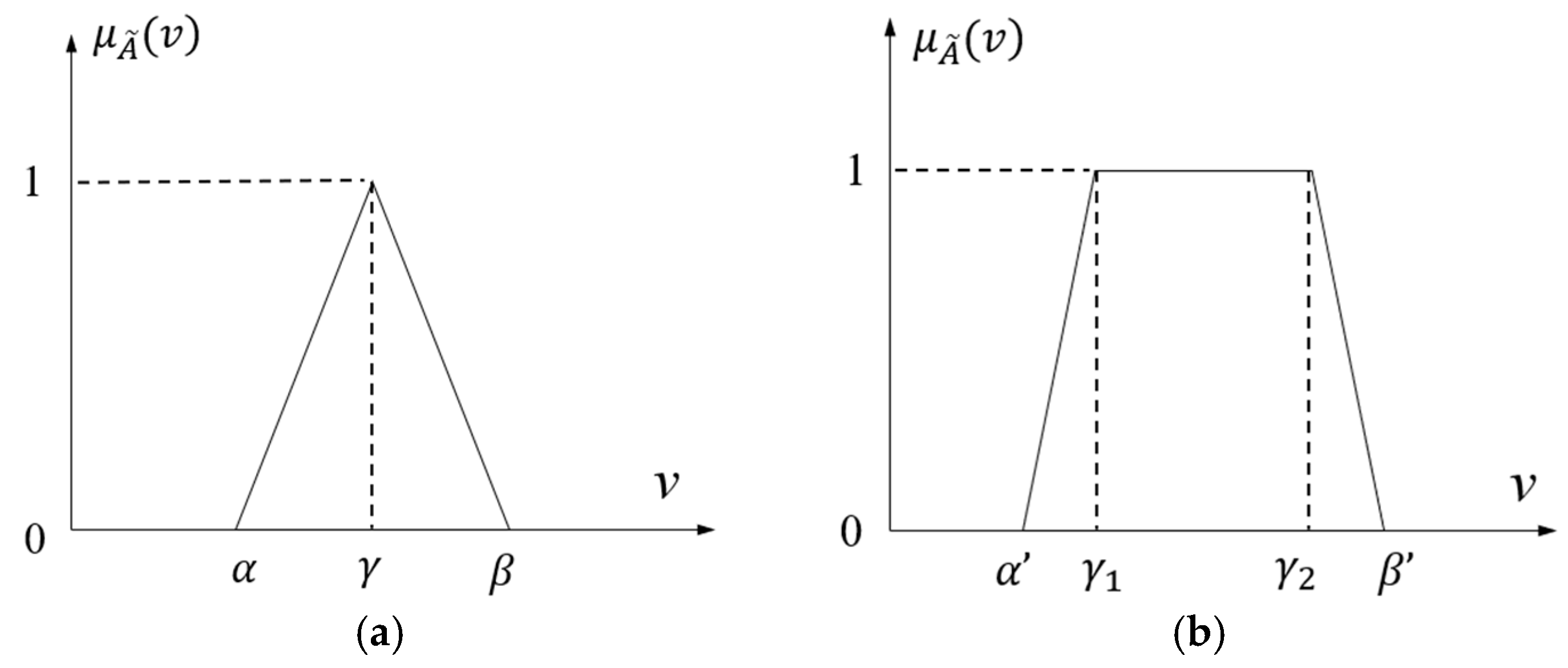
2.3.1. Heading Control Using FLC

As described in the previous section, linear regression fitting is performed on the centers of multiple objects, measured in pixels, to obtain a regression line (see Figure 6). This process can generate up to three regression lines. Additionally, the average heading angle can be calculated using Equation (14):

$$\theta ={\displaystyle \sum _{n=1}^N{\tan }^{-1}{\stackrel{⌢}{a}}_n}/N$$

(14)

where N represents the number of object categories.

Figure 6. Illustration of multiple regression line and heading angle. The dotted line represents the vertical line in the image. The black line signifies the regression line.

In practical operation, these regression lines, constructed from pixel coordinates, are used to estimate their slope. When the guidance line is parallel to any vertical line on the image, this indicates that the robot is moving straight forward without deviating from the desired heading. However, the presence of positive or negative slopes, as well as changes in the slope, typically signify a deviation in the heading to the right or left, respectively.

Fuzzy logic is a well-known technique that involves expert opinion in decision making and is particularly suitable for finding effective solutions when information is insufficient. In this study, an FLC is utilized to adjust the heading angle of the robot. Its components include fuzzification, fuzzy decision making, defuzzification, and a knowledge base [42].

First, the role of fuzzification is to map input crisp values, denoted as “v”, to fuzzy sets. This involves defining a linguistic term $\tilde{A}$ to represent a fuzzy set, viewed as a membership function. The most common membership functions are triangular and trapezoidal. As shown in Figure 7a, the triangular function and its mathematical representation consist of three parameters. The lower boundaries on the left and right are represented by $\alpha$ and $\beta$, respectively, while $\gamma$ denotes the peak of the triangle. When the input crisp value “v” falls between $\alpha$ and $\gamma$, its degree of membership ${\mu }_{\tilde{A}}(v)$ is nonzero, while it is one when “v” equals $\gamma$ and zero when “v” is less than α or greater than β. This implies that the closer “v” is to $\gamma$, the higher its degree of membership. Similarly, Figure 7b depicts the trapezoidal membership function and its mathematical representation, consisting of four parameters: $\alpha \prime$, ${\gamma }_1$, ${\gamma }_2$, and β’.

Figure 7. Illustration of membership function and their mathematical expressions. (a) Triangular membership function. (b) Ladder membership function.

In the FLC, the heading angle (θ) and the rate of change of the heading angle ($\dot{\theta }$) are the two input variables. The heading angle corresponds to three fuzzy linguistic terms: left offset (LO), middle (M), and right offset (RO). Additionally, the rate of change of the heading angle is represented by three fuzzy linguistic terms: negative (N), zero (Z), and positive (P). The output variable is the steering angle (δ), defined by the fuzzy linguistic terms left (L), mid (M), and right (R). Table 1 compiles the input and output variable values, corresponding to the fuzzy logic statements, and the parameter values of their membership functions for the FLC.

Table 1. Parameters of membership function of input and output variables in FLC.

Input Variable						Output Variable
Heading angle (θ)			Rate of change of the heading angle ($\dot{\theta }$)			Steering angle (δ)
Crisp interval		Linguistic labels	Crisp interval		Linguistic labels	Crisp interval		Linguistic labels
Triangular [$\alpha ,\gamma ,\beta$]	Ladderr [${\alpha }^{\prime },{\gamma }_1,{\gamma }_2,{\beta }^{\prime }$]		Triangularr [$\alpha ,\gamma ,\beta$]	Ladderr [${\alpha }^{\prime },{\gamma }_1,{\gamma }_2,{\beta }^{\prime }$]		Triangularr [$\alpha ,\gamma ,\beta$]	Ladderr [${\alpha }^{\prime },{\gamma }_1,{\gamma }_2,{\beta }^{\prime }$]
−	[−100, −100, −20, 0]	LO	−	[−100, −100, −25, 0]	N	−	[−17, −17, −7, 0]	L
[−10, 0, 10]	−	M	[−20, 0, 20]	−	Z	[−5, 0, 5]	−	M
−	[0, 20, 100, 100]	RO	−	[0, 25, 100, 100]	P	−	[0, 7, 17, 17]	R

Second, the knowledge base consists of rules that primarily use [IF—THEN] statements to describe the relationships between the input and output variables. When multiple input variables are involved in the FLC, [IF—AND—THEN] statements are used. In this study, nine rules have been defined based on two input variables (θ and $\dot{\theta }$) and one output variable (δ):

Rule 1:

IF ($\theta$ is LO) AND ($\dot{\theta }$ is N) THEN ($\delta$ is L);

Rule 2:

IF ($\theta$ is LO) AND ($\dot{\theta }$ is Z) THEN ($\delta$ is M);

Rule 3:

IF ($\theta$ is LO) AND ($\dot{\theta }$ is P) THEN ($\delta$ is R);

Rule 4:

IF ($\theta$ is M) AND ($\dot{\theta }$ is N) THEN ($\delta$ is L);

Rule 5:

IF ($\theta$ is M) AND ($\dot{\theta }$ is Z) THEN ($\delta$ is M);

Rule 6:

IF ($\theta$ is M) AND ($\dot{\theta }$ is P) THEN ($\delta$ is R);

Rule 7:

IF ($\theta$ is RO) AND ($\dot{\theta }$ is N) THEN ($\delta$ is L);

Rule 8:

IF ($\theta$ is RO) AND ($\dot{\theta }$ is Z) THEN ($\delta$ is M);

Rule 9:

IF ($\theta$ is RO) AND ($\dot{\theta }$ is P) THEN ($\delta$ is R).

For example, Rule 1 states that when θ belongs to the “left offset” category, and $\dot{\theta }$ indicates a “negative rate of change”, the wheels should turn left.

Subsequently, the fuzzy decision and defuzzification are established. For decision making, the Mamdani model, also known as the “max-min composition method”, is employed. The principle of this model involves selecting the minimum membership degree corresponding to the fuzzy set of the antecedent condition in the activated rules and assigning it to the corresponding fuzzy set in the consequent condition based on the input values (“minimum” operation). The output fuzzy sets of all the activated rules are then combined using a union operation (i.e., the “maximum” operation). After the comprehensive inference, the final result comprises a series of fuzzy sets with varying degrees. For defuzzification, the centroid method is used to convert these fuzzy values into crisp values.

2.3.2. Speed Control Using a PID Controller

The PID controller is commonly used to regulate the speed of a robot. It maintains the stable motion of the robot by adjusting three parameters: the proportional gain ($K_p$), integral gain ($K_i$) and differential gain ($K_d$). When the “P” term increases, the output in response to an error also increases, and vice versa. However, using only the “P” term, the system may exhibit a steady state error. To eliminate this offset, the “I” term was introduced, which works by integrating the error over time to accelerate the system’s response in reaching the target state. As time progresses, the “I” term accumulates, meaning that even with smaller errors, its contribution grows due to the passage of time until the steady state error is eliminated. On the other hand, the “D” term adjusts based on the rate of change of the error relative to time. In this study, four sets of PID controllers were used to control the rotation speed of the four motors of a four-wheeled robot, with each dedicated to one motor. This approach ensures precise adjustments, responding to the specific needs and conditions of each wheel and thereby enhancing the robot’s overall stability and performance in varying operational contexts. The output of the PID controller, denoted as $u(t)$, is calculated as follows:

$$u(t)=\underset{\mathrm{P}}{\underbrace{K_{p}e(t)}}+\underset{\mathrm{I}}{\underbrace{K_i{\displaystyle {\int }_0^{t}e(t)dt}}}+\underset{D}{\underbrace{K_d\frac{d}{dt}e(t)}}$$

(15)

where $e(t)$ represents the error between the desired velocity and estimated velocity at time $t$. The PID parameters are defined in Table 2. Initially, a trial-and-error method is employed to determine the parameter $K_p$ that brings the system to a marginally stable state. This process yields a proportional gain parameter, denoted as $K_{pc}$. $K_{pc}$, in combination with a proportional coefficient, which is used to set the parameter $K_i$. Additionally, the system’s time period, denoted as $T_c$, is measured and employed to obtain the parameter $K_d$.

Table 2. Definition of parameters of PID controller for speed control of a robot.

Parameters	$K_p$	$K_i$	$K_d$
Value	$0.3 K_{pc}$	$0.2 K_{pc}$	$0.06 K_{pc}{T}_c$

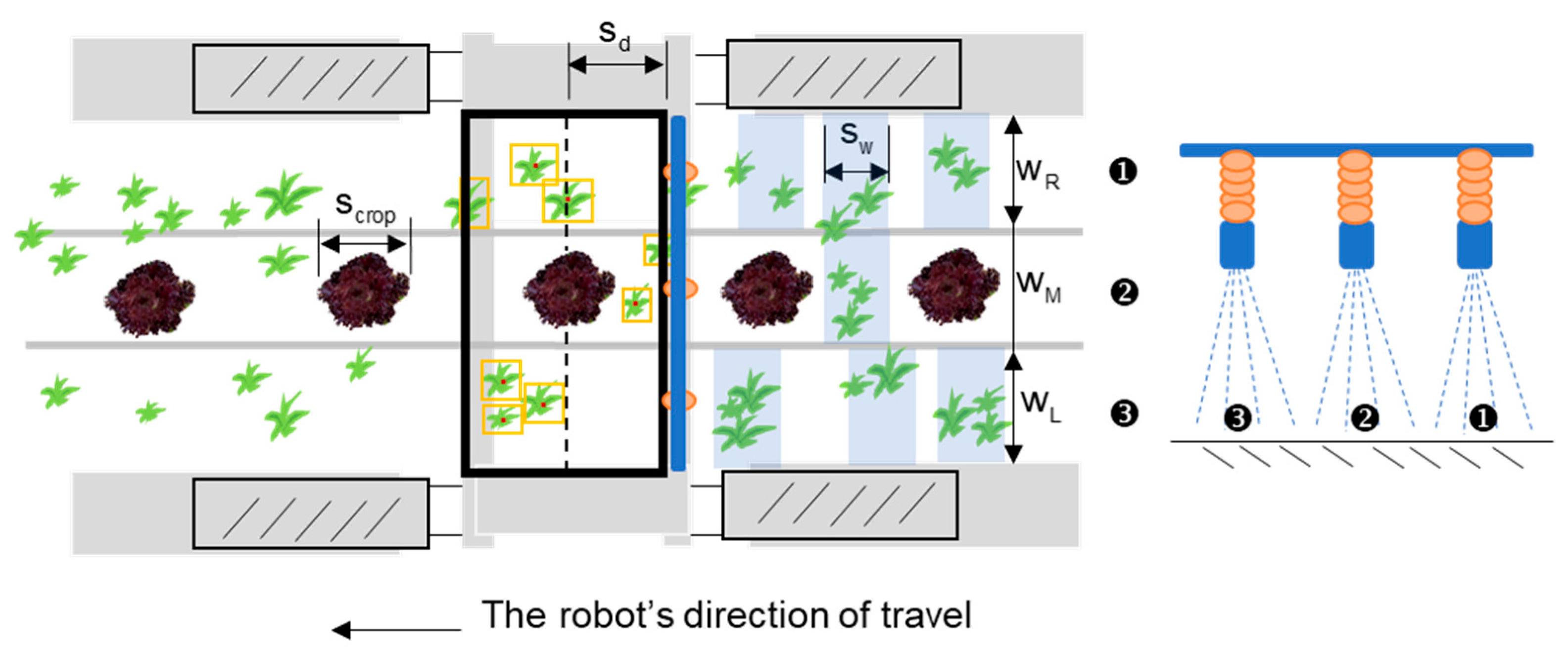
2.4. Selective Spraying

The design concept of selective spraying is depicted in Figure 8. A farm robot carries a camera and three nozzles for dispensing herbicide. The camera is positioned approximately 40 cm above the ground to ensure a comprehensive top-down field of view (depicted as the bold black box in Figure 8). The nozzles are positioned approximately 20 cm above the ground. The spray areas are divided into three sub-areas, represented by the symbols “❶”, “❷”, and “❸”, with each corresponding to a set on the ridge. As mentioned in Section 2.2, the YOLO v4 model was used to detect drip irrigation belts, crops, and field ridges from images. A separate YOLO v4 model is also trained to specifically detect weeds and unhealthy crops, identifying the presence of tiny weeds on the ridge. When weeds or unhealthy crops are detected, the center point position of the object in pixels is estimated. As the robot travels, these tracked center points within the image cross trigger lines on the screen of the camera, as shown by the dotted line in Figure 9, activating the corresponding nozzles to deliver chemicals or nutrient solutions to the targeted objects (weeds or unhealthy crops). The middle nozzle can be used to deliver nutrient solutions or pesticides. It is important to note that the nozzle type and pressure are adjusted to cover their corresponding areas. The distance between the camera and nozzles, denoted as ${\mathrm{s}}_{\mathrm{d}}$, is crucial. When the sprayer is active, the center point of the object now crossing the spray line can be ignored to reduce the possibility of spray failure. During spraying, the distance traveled by the robot can be regarded as ${\mathrm{s}}_{\mathrm{w}}=v{t}_s$, where $t_s$ represents the spraying time. Light blue indicates the sprayed areas, and ${\mathrm{w}}_{\mathrm{R}}$, ${\mathrm{w}}_{\mathrm{M}}$, and ${\mathrm{w}}_{\mathrm{L}}$ denote the width of the right-hand, middle, and left-hand ridge in cm, respectively.

Figure 8. Design concept of selective spraying based on deep learning for an agricultural robot (depicted in gray color) in the field. Symbols “❶”, “❷”, and “❸” represent the right, middle, and left spray areas, respectively, each corresponding to one of the three nozzles. Purple color indicates lettuce; green color signifies weeds; and light blue color denotes areas that have been sprayed.

Figure 9. The experimental platform of a farming robot. Key components are labeled as follows: ❶ = two GNSS antennas; ❷ = control box; ❸ = installation space of spraying module; ❹ = linear electric actuator; ❺ = battery; ❻ = DC blushless motor; and ❼ = water tank.

In practice, the nozzles deliver chemicals to the weeds as soon as the center point of a detected weed object crosses the spray line. Due to varying weed sizes and dispersion of weeds, the object detector, even with lower recognition ability, still ensures that most of the weeds are covered with herbicides. The relationship between $t_s$, the width of the object ${\mathrm{s}}_{‘\mathrm{object}’}$, the delay time for starting the sprayer $t_{delay}$, and the speed of the robot $v$ is as follows:

$$s_d-\lambda {\mathrm{s}}_{‘\mathrm{object}’}<(t_s+t_{delay})v<s_d+(1-\lambda ){\mathrm{s}}_{‘\mathrm{object}’}$$

(16)

where $0\le \lambda < 1$ is the regulation factor and $\mathrm{object}\in (\mathrm{crop}, \mathrm{weed})$. Two evaluation metrics, the effective weed coverage (EWC) and ineffective weed coverage (IWC), are used to evaluate the coverage area of effective spraying and the area of ineffective spraying, given a known weed detection rate. It is assumed that there are three nozzles with fixed heights and arrangements:

$$\mathrm{EWC} (\%)=\frac{{\mathrm{N}}_{{\mathrm{T}}_{\mathrm{R}}}{\mathrm{s}}_{\mathrm{w}}{\mathrm{w}}_{\mathrm{R}}+{\mathrm{N}}_{{\mathrm{T}}_{\mathrm{M}}}{\mathrm{s}}_{\mathrm{w}}{\mathrm{w}}_{\mathrm{M}}{+\mathrm{N}}_{{\mathrm{T}}_{\mathrm{L}}}{\mathrm{s}}_{\mathrm{w}}{\mathrm{w}}_{\mathrm{L}}}{{\mathrm{L}(\mathrm{w}}_{\mathrm{R}}+{\mathrm{w}}_{\mathrm{M}}{+\mathrm{w}}_{\mathrm{L}})-{\mathrm{s}}_{\mathrm{crop}}{\mathrm{w}}_{\mathrm{M}}}$$

(17)

$$\mathrm{IWC} (\%)=\frac{{\mathrm{N}}_{{\mathrm{F}}_{\mathrm{R}}}{\mathrm{s}}_{\mathrm{w}}{\mathrm{w}}_{\mathrm{R}}+{\mathrm{N}}_{{\mathrm{F}}_{\mathrm{M}}}{\mathrm{s}}_{\mathrm{w}}{\mathrm{w}}_{\mathrm{M}}+{\mathrm{N}}_{{\mathrm{F}}_{\mathrm{L}}}{\mathrm{s}}_{\mathrm{w}}{\mathrm{w}}_{\mathrm{L}}}{{\mathrm{L}(\mathrm{w}}_{\mathrm{R}}+{\mathrm{w}}_{\mathrm{M}}{+\mathrm{w}}_{\mathrm{L}})-{\mathrm{s}}_{\mathrm{crop}}{\mathrm{w}}_{\mathrm{M}}}$$

(18)

where L represents the total length of the selective spraying experimental site and ${\mathrm{N}}_{{\mathrm{T}}_{\mathrm{R}}}$, ${\mathrm{N}}_{{\mathrm{T}}_{\mathrm{M}}}$, and ${\mathrm{N}}_{{\mathrm{T}}_{\mathrm{L}}}$ represent the number of times the right, middle, and left nozzles correctly deliver the pesticide to the weeds, respectively. Conversely, ${\mathrm{N}}_{{\mathrm{F}}_{\mathrm{R}}}$, ${\mathrm{N}}_{{\mathrm{F}}_{\mathrm{M}}}$, and ${\mathrm{N}}_{{\mathrm{F}}_{\mathrm{L}}}$ represent the number of times the right, middle, and left nozzles incorrectly deliver the pesticide, respectively. These values are estimated through spray control systems and experiments. It is particularly noteworthy that the process of spraying unhealthy crops is distinct from that of spraying weeds. The spraying rate $\mathrm{sprayC} (\%)={\mathrm{N}}_{\mathrm{U}}/{\mathrm{N}}_{\mathrm{C}}$ is used to evaluate the spraying efficiency, where ${\mathrm{N}}_{\mathrm{U}}$ and ${\mathrm{N}}_{\mathrm{C}}$ represent the number of sprayed unhealthy crops and the actual number of unhealthy crops, respectively. Finally, the amount of pesticide consumed by selective spraying ${\mathrm{C}}_{\mathrm{sel}}$ and the amount of traditional spraying ${\mathrm{C}}_{\mathrm{full}}$ are compared to determine the pesticide reduction ratio $\mathrm{C} (\%)={{(\mathrm{C}}_{\mathrm{full}}-{\mathrm{C}}_{\mathrm{sel}})/\mathrm{C}}_{\mathrm{full}}$.

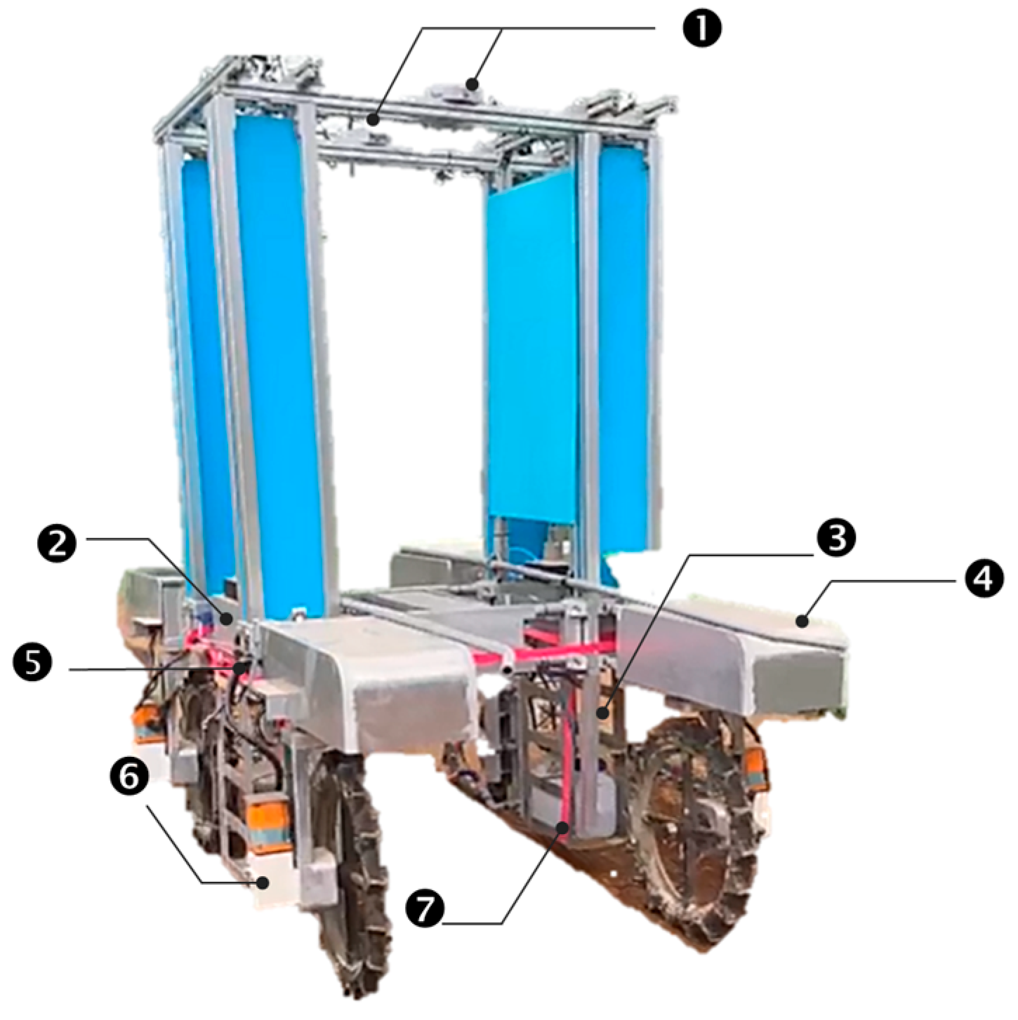
3. Description of the Farming Robot

A four-wheel-drive (4WD) and four-wheel-steering (4WS) farming robot was utilized to evaluate the autonomous navigation and selective spraying with deep learning approach. The mechanism of the robot and software and hardware system configuration are explained below.

3.1. Mechatronics System

The experimental platform, shown in Figure 9, features a chassis composed of multiple modular mechanical components [43]. The height of the robot is available in two types: 80 cm and 200 cm. Its width is adjustable through a platinum connecting element. The shock absorber, forming a double A-arm shock absorber module, is 21 cm long with a 4 cm compression stroke. The wheels, made of hard rubber, have a diameter of 65 cm and a width of 8 cm. Each wheel is powered by a DC brushless motor (model: 9B200P-DM, TROY Enterprise Co., Ltd., Wugu, New Taipei City, Taiwan) coupled to a reduction gear set (model: 9VD360H, TROY Enterprise Co., Ltd., Wugu, New Taipei City, Taiwan) with a 360:1 reduction ratio and controlled by a motor drive (model: AGV-BLD-1S-200W, TROY Enterprise Co., Ltd., Wugu, New Taipei City, Taiwan). Additionally, four steering drives (model: CSBL1400, CSIM Inc., Xinzhuang, New Taipei City, Taiwan) are connected to four servo motors (model: CS60-150C8AE, CSIM Inc., Xinzhuang, New Taipei City, Taiwan) built into linear electric actuators (model: LOE-40-100-C-L5, LIND Inc., Taiping, Taichung County, Taiwan). The robot’s embedded board and peripheral electronic components are housed inside a control box. Two sets of RTK-GNSS modules (model: C099-F9P, u-Blox Inc., Thalwil, canton of Zürich, Switzerland) with two antennas (model: VEXXIS Antennas GNSS-502, NovAtel Inc., Issy-les-Moulineaux, France) are installed on the front and rear brackets at the top of the robot. An embedded board (model: Jetson Xavier NX, NVIDIA Inc., Sunnyvale, CA, USA), serving as the main controller of the robot’s operating system, executes deep learning algorithms for selective spraying and enables autonomous operation based on programmed instructions. A camera (model: BRIO 4K Ultra HD, Logitech Inc., Lausanne, Switzerland) is mounted under the central frame to capture images of field ridges, crops, weeds, or drip irrigation belts. The spray module, housed in a waterproof box attached to the side bracket, is connected by hoses to nozzles at the rear of the central bracket. The nozzles, directed toward the ground, cover the left, center, and right areas of the camera’s field of view. Data transfer connectivity utilizes Universal Serial Bus (USB), General-Purpose Input/Output (GPIO), RS485, and RS-232 protocols, providing an interface between the robot’s operating system and electronic components such as the camera, GNSS receivers, drivers, spraying module, and other peripherals (Figure 10). The detailed specifications of the electronic components are presented in Table 3.

Figure 10. Hardware architecture of robotic control system.

Table 3. Component specification for an agricultural robot.

Description	Value or Other Details
Mechanism body
Length	2.4 m
Width	1.06 m
Height	2 m
Wheel diameter	0.65 m
Maximum weight	440 kg
Drive components
Drive method	4 WS/4 WD
Maximum speed	1 Km/h
Motors (input voltage, gear ratio; torque)	DC 24 V, 1/360, 0.8 N-m
Linear electric actuator (input voltage, gear ratio; torque)	DC 24 V, 1/5, 0.64 N-m
Battery (voltage, capacity)	DC 24 V, 30 Ah
Sprayer
Electromagnetic valve (volt, pressure)	DC 12 V, 0~10 Kg/cm2
Pump (input voltage, power, pressure, volumetric flow rate)	DC 24 V, 70 W, 1.0 MPA, 4.5 L/min
Copper nozzle (diameter)	1 mm/0.1 mm
Water container	20 L
Electronics
GNSS receiver (voltage, accuracy, band)	3.3/5 V, 0.01 m–2.5 m, L1/L2C
Antennas (input voltage, signal type, noise figure, type, connector)	3.3 V–18 V, GPS/GLONASS/Galileo/BeiDou, 2.5 dB, active, TNC
Camera (maximum resolution, mega pixel, focus type, FoV, connection type)	4 K/30 FPS, 13, autofocus, 90 degree, USB

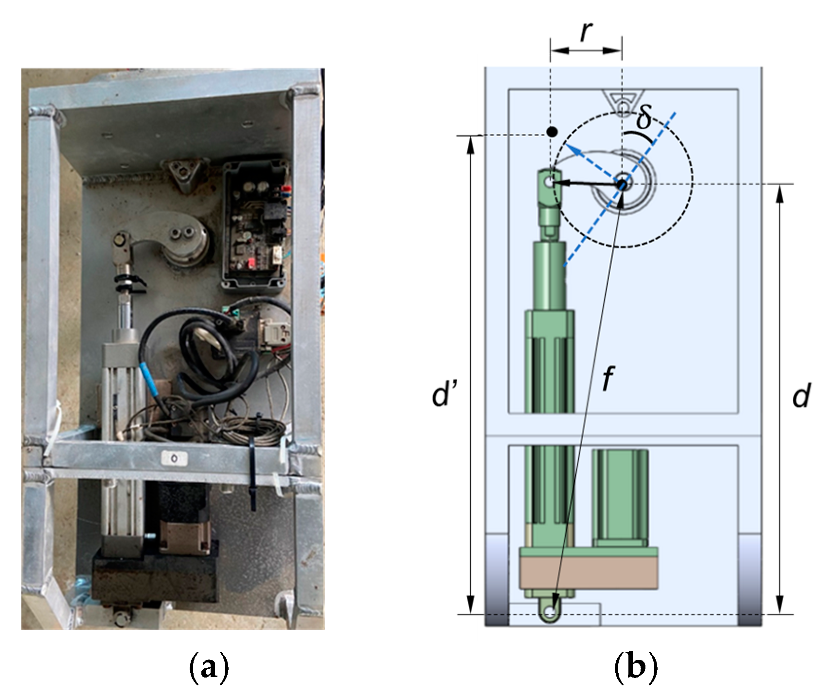
3.2. Steering Mechanism

The linear electric actuator, characterized by its high output torque, is ideally suited for assembly in agricultural robots, particularly for steering control. It comprises a servo motor and a screw mechanism, which convert the rotational motion of the motor shaft into the linear motion of the piston rod. This steering mechanism is used to adjust the steering angle δ (as shown in Figure 11), which is defined by Equation (19):

$$\delta ={\cos }^{-1}\left(\frac{r^2+f^2-d{\prime }^2}{2rf}\right)-{\cos }^{-1}\left(\frac{r^2+f^2-d^2}{2rf}\right)$$

(19)

where $r$ denotes the length from the center point of the link slider to the endpoint of the piston rod and f represents the distance between the center point of the link slider and the base end of the electric actuator, while $d$ and $d^{\prime }$ signify the original length and the extended length from the front end to the base end of the electric actuator, respectively. In this study, $r$ = 8.07 cm, $f=46.8 \mathrm{cm}$, and $d=39.6 \mathrm{cm}$.

Figure 11. Steering mechanism of robot. (a) Appearance of steering mechanism. (b) Relationship between the steering and linear electronic actuators.

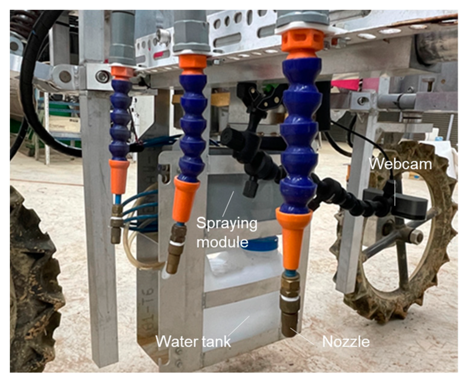
3.3. Spraying Module

The circuit of the spray module is shown in Figure 12a. The main controller operates the spray program and sends a start or stop command to the relay module through the GPIO interface. This process controls the activation or deactivation of the solenoid valve, thereby regulating the timing of the spraying. A webcam is utilized to capture images on the ridge. The control box, shown in the upper part of Figure 12b, includes relays, DC-DC converters, transformers, and peripheral circuit components. The internal components of the spray box, depicted in the lower part of Figure 12b, comprise pumps, solenoid valves, connectors, and plastic water pipes. Five sets of spray connectors are installed on both the left and right sides of the box. Both the external appearance and the internal configuration of the spray nozzle used in the agricultural robot are shown in Figure 13.

Figure 12. Spray module. (a) A diagram illustrating the spraying circuit. (b) The internal configuration of the control box showing peripheral components (top) and the arrangement of water pipe connections inside the spray box (bottom).

Figure 13. The external appearance and the internal configuration of the spray nozzle.

4. Experiments and Results

4.1. Environmental Conditions and Parameters

The experimental site was an empty field located in front of the Department of Biomechanical Engineering building (longitude: 120.6059°, latitude: 22.6467°). The experiments were conducted from summer to autumn. The field spans approximately 10 m in length, with individual ridge widths measuring 80 cm. Due to the limited farming area, we only allowed the farming robot to move between two ridges (as shown in Figure 14). The experimental site is surrounded by green trees. The left and right wheels of the robot straddled the sides of a strip-shaped farmland, with both ends of the farmland serving as turning points (marked by star-shaped dots). When the position of the robot fell into the set range to be turned, the robot stopped and performed a 90 degree on-the-spot rotation in place to keep the head of the robot facing the forward direction. The motion behavior was repeated until the robot returned to the origin point (see “ST/END” in Figure 14).

Figure 14. Schematic of movement behavior of the robot in the field. Star-shaped dots represent turning points, as well as start and end (ST/END) points.

The GNSS receiver, enhanced with RTK capabilities, produces navigation data in a format established by the National Marine Electronics Association (NMEA), offering highly accurate longitudinal and latitudinal details [44]. Two GNSS receivers were employed to record the robot position, separated by 0.65 m. The latitude and longitude of the location obtained from the two receivers were each converted into two TWD97-based positions [45]. Generally speaking, a typical video frame rate is 15–30 FPS [46]. Considering hardware limitations and expected objects, in this study, FPS values between 1 and 13 were evaluated with an image size of 416 × 416.

The experimental periods were divided into morning (9:00–11:00 a.m.), noon (12:00–2:00 p.m.), and afternoon (3:00–5:00 p.m.). The weather conditions during these periods varied and may have been sunny (9800~35,000 lux), partly sunny (3000~9800 lux), or cloudy (0~3000 lux). The experimental period spanned 3 months. Since lettuce crops are harvested approximately 20–30 days after sowing, a total of three harvests were performed during the trial, and the cultivated land was reseeded after each harvest. During the planting process, the amount of watering for each crop was adjusted, resulting in differences in growth conditions.

4.2. Preliminary Test

Red leaf lettuce (model: HV-067, Taiwan Known-You Seed Co., Ltd., Dashu Kaohsiung city, Taiwan) was selected as the target crop. Two YOLO v4 models were trained and employed for guidance line detection (DetModel #1) and the detection of weeds and unhealthy crops (DetModel #2). The users captured image samples randomly at the experimental site every day using cameras. These images encompassed weeds, both healthy and abnormal crops, drip irrigation belts, and ridges.

A total of 5800 images were collected in the experimental farm area of Pingtung University of Science and Technology during the autumn and winter of 2023. A multi-channel data logger (model: WatchDog 1650, Spectrum Technologies, Inc., Aurora, IL, USA) was used to record the light intensity. These images were taken through the camera on the robot platform at different times and under different weather conditions. Each image showed drip irrigation belts, field ridges, crops, unhealthy crops, or weeds. These images were then processed through image argumentation to obtain a total of 9500 images, which were used to build DetModel #1 and DetModel #2. The images were divided into a training set, test set, and validation set according to the ratio of 7:2:1. The images in the training set were manually annotated by using the open-source image annotation tool LabelImg to mark objects within the images. The abnormal growth of crops was characterized by symptoms such as wrinkled leaves, as depicted in Figure 15a,b. The type of weed at the experimental site is also shown in Figure 15c.

Figure 15. Leaf appearance for unhealthy crops and weeds. (a) Wrinkled leaves (sample 1). (b) Wrinkled leaves (sample 2). (c) The type of weed.

The hyperparameters for both YOLO v4 models (DetModel #1 and #2) were configured as follows: the batch size set to 64, subdivisions set to 32, image size of 416 × 416 (width × height), decay rate of 0.0005, momentum of 0.949, learning rate set to 0.001, and maximum number of batches set to 10,000.

The training iterations for DetModel #1 and DetModel #2 were stopped after reaching 10,000 and 6000 iterations, with $P_{Loss}$ values of 1.0719 and 14.8856, respectively. The mean average precision (mAP) values of DetModel #1 and DetModel #2 were 99.0% and 92.7%, respectively (Figure 16).

Figure 16. Identification of objects in the ridge using trained YOLO v4 models. (a) Detection results for the ridge, drip irrigation belt, and crops using DetModel #1. (b) Detection results for weeds and unhealthy crops using DetModel #2, featuring weed detection results (purple bounding box on the left side), the loss convergence curve (in the middle), unhealthy crops (green box on the right side), and weeds (purple bounding box).

The performance comparison results of the two detection models, DetModel #1 and DetModel #2, under different weather conditions are shown in Table 4. The results indicate that the recognition rates of DetModel #1 for detecting drip irrigation belts, crops, and ridges ranged from about 96 to 99%, 93 to 98%, and 93 to 97% respectively. Under the sunny conditions and during time periods from 3:00 to 5:00 p.m., DetModel #1 achieved the best recognition rate of 99% for identifying drip irrigation belts. On cloudy days and between 3:00 and 5:00 p.m., the average precision for ridges dropped to 93%. Overall, using DetModel #1, the average accuracy was about 98%. Secondly, the accuracy of DetModel #2 for detecting unhealthy crops and weeds ranged from 84 to 92% and 86 to 92%, respectively. Among these, the highest accuracy rate for weed detection was 93% on sunny days between 9:00 and 11:00 a.m. In contrast, on cloudy days during the same time period, the detection rate fell to 84%. Using DetModel #2, the average accuracy for weeds and unhealthy crops was about 88%.

Table 4. Comparison of the performance of detection models in identifying different types of objects under different weather conditions.

Name of Model	Type of Object	Evaluation Matric (%)	Sunny			Partly Sunny			Cloudy
			9:00~ 11:00 a.m.	12:00~ 2:00 p.m.	3:00~ 5:00 p.m.	9:00~ 11:00 a.m.	12:00~ 2:00 p.m.	3:00~ 5:00 p.m.	9:00~ 11:00 a.m.	12:00~ 2:00 p.m.	3:00~ 5:00 p.m.
DetModel #1	Drip irrigation belt	PR	98.1 ± 0.1	94.3 ± 0.7	98.7 ± 0.9	97.3 ± 0.9	94.3 ± 0.9	97.2 ± 0.9	97.2 ± 0.3	95.1 ± 0.4	96.4 ± 0.7
		Recall	96.2 ± 0.5	94.3 ± 0.8	97.4 ± 0.9	95.1 ± 0.8	94.1 ± 1.1	96.6 ± 0.7	96.1 ± 0.5	93.7 ± 0.6	94.7 ± 0.6
		F1 score	97.1 ± 0.1	94.3 ± 0.7	98.0 ± 0.9	96.2 ± 0.8	94.2 ± 0.9	96.9 ± 0.8	96.6 ± 0.4	94.4 ± 0.5	95.5 ± 0.6
	Crop	PR	97.8 ± 0.2	93.2 ± 0.5	97.6 ± 0.1	97.8 ± 0.9	94.3 ± 1.1	97.1 ± 1.0	97.8 ± 0.7	95.0 ± 0.8	97.4 ± 0.3
		Recall	96.1 ± 0.1	93.1 ± 0.7	96.9 ± 0.4	96.8 ± 0.6	94.6 ± 0.9	96.7 ± 0.8	96.1 ± 0.6	94.1 ± 0.6	96.3 ± 0.3
		F1 score	96.9 ± 0.1	93.1 ± 0.6	97.2 ± 0.3	97.3 ± 0.7	94.4 ± 1.0	96.9 ± 0.9	96.9 ± 0.6	94.5 ± 0.7	96.8 ± 0.3
	Ridge	PR	95.3 ± 0.2	93.4 ± 0.8	97.1 ± 0.9	95.2 ± 1.1	94.3 ± 1.2	96.9 ± 1.1	94.8 ± 0.3	94.2 ± 0.9	93.2 ± 1.2
		Recall	96.1 ± 0.4	95.1 ± 0.7	96.1 ± 0.6	94.7 ± 0.7	94.4 ± 0.1	96.8 ± 0.8	94.1 ± 0.2	94.2 ± 0.7	93.3 ± 0.2
		F1 score	95.7 ± 0.3	94.2 ± 0.7	96.6 ± 0.7	94.9 ± 0.9	94.3 ± 0.2	97.2 ± 0.9	94.4 ± 0.2	94.2 ± 0.7	93.2 ± 0.3
DetModel #2	Unhealthy crop	PR	90.3 ± 2.0	88.3 ± 2.2	91.2 ± 1.8	90.1 ± 0.5	87.8 ± 1.2	90.8 ± 1.2	90.2 ± 1.1	88.4 ± 1.8	85.1 ± 1.4
		Recall	81.3 ± 0.1	82.4 ± 0.1	82.4 ± 0.1	83.1 ± 0.4	83.2 ± 0.9	82.2 ± 0.9	81.1 ± 1.0	81.3 ± 1.2	80.3 ± 1.1
		F1 score	85.6 ± 0.2	85.2 ± 0.2	86.4 ± 0.2	86.5 ± 0.4	85.4 ± 0.9	86.3 ± 0.9	85.4 ± 1.1	84.7 ± 1.3	82.6 ± 1.2
	Weed	PR	92.1 ± 1.1	88.3 ± 1.5	90.1 ± 1.8	89.7 ± 1.4	90.8 ± 1.2	90.2 ± 1.9	90.2 ± 1.1	88.7 ± 1.2	86.6 ± 1.5
		Recall	84.3 ± 0.1	81.2 ± 1.1	82.4 ± 1.6	83.4 ± 1.3	84.1 ± 1.1	82.4 ± 1.6	83.3 ± 0.9	82.4 ± 1.0	80.3 ± 1.1
		F1 score	88.0 ± 0.2	84.6 ± 1.1	86.1 ± 1.6	86.4 ± 1.3	87.3 ± 1.1	86.1 ± 1.7	86.6 ± 0.9	85.4 ± 1.1	83.3 ± 1.1

4.3. Experimental Results

Two scenarios, comprising the autonomous guidance and selective spraying experiments, were conducted to evaluate the robustness of the proposed scheme.

4.3.1. Scenario 1

A total of 60 crops were planted in two rows of farmland. The speed of the robot was 12.5 cm/s. During the autonomous navigation of the farming robot, data such as the velocity of each motor, heading angle, and the output value of the FLC were recorded. The experimental time was from 9:00 to 11:00 a.m., and the weather conditions were sunny. Three types of guidance lines were measured to estimate the deviation angle (N = 3), and the angles were averaged to determine the real-time heading angle of the robot. PID control and a fuzzy logic-based steering control program embedded in the guidance system were executed to continuously maintain the speed of the robot and correct its heading angle. The movement trajectory of the robot was obtained by two GNSS receivers as shown in Figure 17a. The change in velocity of each wheel of the robot is shown in Figure 17b. The control parameters of the PID controller for the four motor drivers, $K_p$, $K_i$, and $K_d$, were all set to 0.5, 0.1, and 0.6, respectively. Specifically, when the robot moved forward, the required motor speed for the four wheels was maintained at approximately 700 rpm (regardless of the reduction ratio). A speed overshoot occurred briefly when the motor speed value was switched. Additionally, this phenomenon also occurred when the velocity of the four motors was maintained at about 1000 rpm during in-place rotation for the robot.

Figure 17. The velocity control of the farming robot in the farmland using PID control. (a) The movement trajectory of the robot (depicted by blue and green dotted lines) obtained using two GNSS receivers. (b) A comparison of the speed variation range and motion behavior of each wheel in relation to the positioning trajectory shown in (a). Numbers 1 through 8 correspond to the respective rotational speed changes of the four motors when the robot is in motion.

Secondly, the results of using different guidance lines for estimating the heading angle and correcting it through the FLC were compared, as shown in Figure 18a. The speed of the robot was 12.5 cm/s. The changes in the heading angles, measured from the regression lines generated by fitting different types of objects, were observed. It was found that when the crop line was used as the reference guidance line, it showed the largest change in heading angle (Figure 18a). Conversely, using the irrigation line as a guidance line resulted in minimal variation in the heading angle. Figure 18b shows the steering angle obtained by using the FLC when the crop line was the guidance line. The output value of the FLC ranged between ±2 degrees, with a few output values reaching ±6 degrees. These larger steering angle peaks appeared within the unit time range of 50~60, 120~130, or 225~235. These values reflect the heading angle and its changes during the corresponding time intervals when the robot traveled along the crop line (Figure 18a). The reason for these instantaneous changes in angles is that the planting position of the crops was deviated due to human factors, or crops that were not growing well (elongated) caused the center point of the labeled object to deviate too far from the expected position.

Figure 18. Changes in heading angle using different types of guidance lines. (a) The average angular variation in the heading angle was approximately 1 degree, indicated by the orange square. (b) The steering angle obtained using the FLC when the crop line served as a navigation line.

On the other hand, the impact of different speeds of the robot on the fitting results of the regression under varying weather conditions was observed. As shown in Figure 19, it is evident that the use of DetModel #1 enabled object detection and achieved a mean average precision (mAP) of 97% when the speed of the robot was 12.5 cm/s. However, as the speed of the robot increased, the mAP gradually decreased. Specifically, at a speed of 19 cm/s, the mAP dropped to below 75%, and when the speed of the robot reached 35 cm/s, the mAP decreased to below 50%. At a travel speed of 12.5 cm/s, there was no significant difference in the mAP under different weather conditions.

Figure 19. Comparison of the robot’s object detection performance at different robot speeds.

A snapshot of the results from using DetModel #1 to continuously detect objects of different categories (FPS = 7) and using the least squares method to generate guidance lines under different weather conditions is shown in Figure 20. Although Figure 20a,b displays an uneven brightness distribution, three lines were still generated: the irrigation line (red), the crop line (orange), and the field border line (blue). The same results were also observed in low-brightness environments, as demonstrated in Figure 20c.

Figure 20. Snapshots showcasing guidance line generation and object detection results under various weather conditions (FPS = 7; speed = 12.5 cm/s). (a) Sunny weather. (b) Partly sunny conditions. (c) Cloudy conditions. Black line represents the vertical line in the center of the image; orange line indicates crop line; red line denotes irrigation line; blue line signifies ridge line; and green frame highlights the detected object frame.

A guidance line was generated after fitting the measured data through least squares regression. The effect of the number of FPS on the reliability of regression line generation was evaluated. Videos recorded by remotely controlling the robot while it traveled at different speeds in the field were used to evaluate the impact of different frame rates on changes in the heading angle. The heading angles obtained from the three fitted regression lines were averaged and compared with the FPS values. When the speed of the robot was maintained at 12.5 cm/s, and the FPS was greater than seven, the variation range in heading angle was about two degrees (Figure 21). Similar results were also presented when the speed of the robot was equal to 19 cm/s and the FPS was equal to 11 and 13. When the speed of the robot was maintained at 24 cm/s, and the FPS was greater than 5, its heading angle changed by about 3.5–5.5 degrees. When the robot speed was 35 cm/s, the FPS had to be increased to above nine to obtain the heading angle. However, in this case, the range of variation in the heading angle was the largest compared with other scenarios.

Figure 21. Variation range in heading angle versus FPS. The heading angle could not be obtained when the speed of the robot was 19 cm/s, 24 cm/s, or 35 cm/s.

4.3.2. Scenario 2

In the selective spraying experiment, water-soluble pigments were used as the spraying solution. After each spraying experiment, weeds were removed manually. About a week later, once the weeds had regrown, the spraying experiment was carried out again. Equations (16) and (17) were used to estimate the EWC and IWC, respectively. The realism of the sprayed area was determined by visually inspecting whether water dripped onto the weeds or crops. This procedure was executed in three replicates, where the total amount of solution applied in each test was quantified through a water storage bucket on the side of the robot.

According to the weed detection results presented in Table 4, the weather conditions during this experiment were sunny, and the time period was from 9:00 to 11:00 a.m. There were two strips of cultivated land. Among them, ${\mathrm{w}}_{\mathrm{R}}{=\mathrm{w}}_{\mathrm{L}}=12 \mathrm{cm}$, ${\mathrm{w}}_{\mathrm{M}}=15 \mathrm{cm}$, ${\mathrm{s}}_{\mathrm{d}}=35 \mathrm{cm}$, and ${\mathrm{s}}_{\mathrm{crop}}=12 \mathrm{cm}.$ When the speed of the robot was 12.5 cm/s, 19 cm/s, 24 cm/s and 35 cm/s, the delay time for starting the sprayer was set to 2.5 s, 1.5 s, 1 s, and 0.5 s, respectively. The spray time of the sprayer was set to 0.5 s ($t_s=0.05$) for each operation. When the spraying program was executed in the robot operating system, it recorded the number of executions of the left, middle, and right nozzles, estimated the spraying area and volume, and compared them with the volume obtained using traditional spraying methods to calculate the pesticide reduction. It is important to note that during the weeding spraying experiments, the robot was remotely controlled by a human at a constant speed, and only the central nozzle sprayed the weeds. Unhealthy crops were not sprayed during these experiments. A windless environment was ensured when performing the spray tests.

The impact of different FPS values on the detection performance of DetModel #2 for weeds and unhealthy crops was also evaluated, with the speed of the robot set to 12.5 cm/s. Figure 22 shows that when the FPS was greater than seven, the average accuracy of detecting weeds and unhealthy crops ranged from 89% to 92% and from 88% to 90%, respectively. However, when the FPS was less than seven, the accuracy of detecting weeds and unhealthy crops dropped significantly.

Figure 22. Comparison of the detection accuracy for weeds and unhealthy crops at different FPS values.

The results for the EWC, IWC, and pesticide reduction rate at different robot speeds with a detection time of 143 ms per image for DetModel #2 are illustrated in Table 5. Pesticide reduction refers to the decrease in pesticide usage achieved by selective spraying compared with traditional uniform spraying. It can be seen from this table that as the speed of the robot increased, the EWC gradually decreased, and the IWC gradually increased. However, limited by the detection performance of DetModel #2, when the robot speed reached 35 cm/s, the EWC was at its lowest, and the IWC was at its highest. In this scenario, although pesticide usage was significantly reduced (about 63%), most weeds were not sprayed.

Table 5. Comparison of effective and ineffective weeding coverage and pesticide reduction rates at different robot speeds ($t_s=0.5$ s).

Speed	EWC (%)	IWC (%)	Pesticide Reduction (%)
12.5 cm/s	82.9 ± 1.9	8.4 ± 0.9	53.2 ± 2.9
19 cm/s	73.0 ± 2.8	15.2 ± 1.9	36.1 ± 3.6
24 cm/s	73.3 ± 5.3	19.4 ± 4.2	30.7 ± 3.6
35 cm/s	23.7 ± 5.3	27.3 ± 5.2	63.4 ± 5.8

The performance of selective spraying for unhealthy crops was evaluated. Each spray time of the sprayer was also set to 0.5 s ($t_s=0.5$ s). The delay time for starting the sprayer was the same as that in the weed spraying experiment. This spraying experiment was conducted at different time periods and under different weather conditions, with the experimental procedures for each time period being repeated three times. The comparison results of the spray rate of the robot at different speeds are demonstrated in Figure 23. When the speed of the robot was 12.5 cm/s, 19 cm/s, 24 cm/s, and 35 cm/s, the spraying rates (SprayC) were between about 85 and 92%, 83% and 88%, 70 and 88%, and 40 and 65%, respectively. A snapshot of an unhealthy crop after spraying is shown in Figure 24. These images were all captured by cameras after selective spraying tests under different weather conditions. The bounding boxes in these images were labeled offline with DetModel #2 and confirm the spray behavior on unhealthy crops or weeds.

Figure 23. Comparison of spray rates (SprayC) for the robot at different speeds and FPS values: (a) 12.5 cm/s; (b) 19 cm/s; (c) 24 cm/s; and (d) 35 cm/s.

Figure 24. Spraying results under different weather conditions (speed of 12.5 cm/s; FPS = 7): (a) sunny (zoomed in); (b) partly sunny; (c) cloudy (Example 1); and (d) coludy (Example 2). The bounding boxes were marked by DetModel #2 after spraying.

4.4. Discussion

Based on the comprehensive analysis of our experimental results, we have summarized the following points:

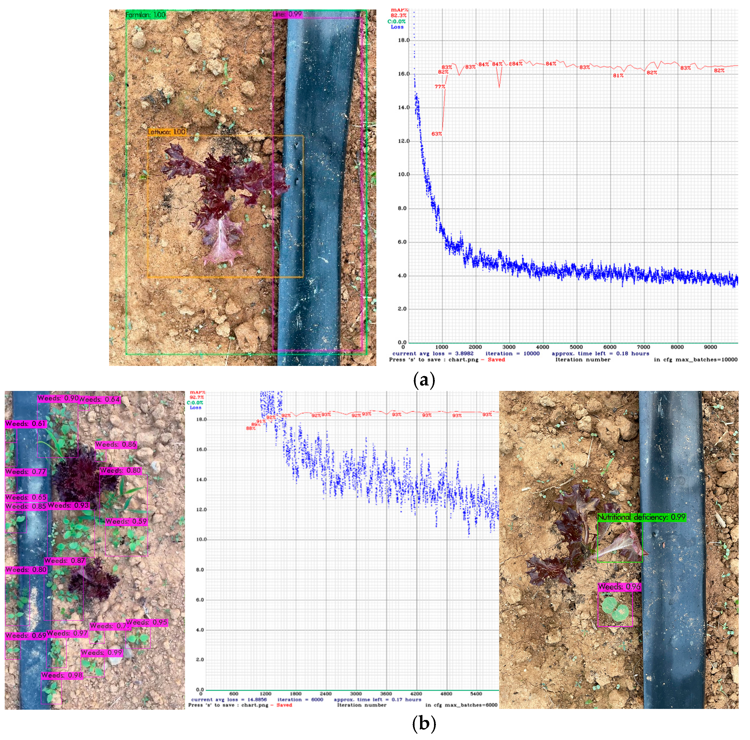
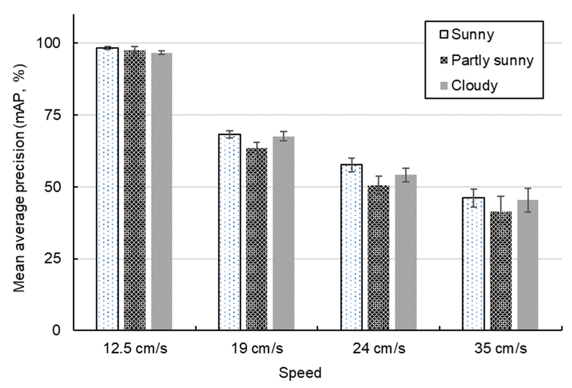
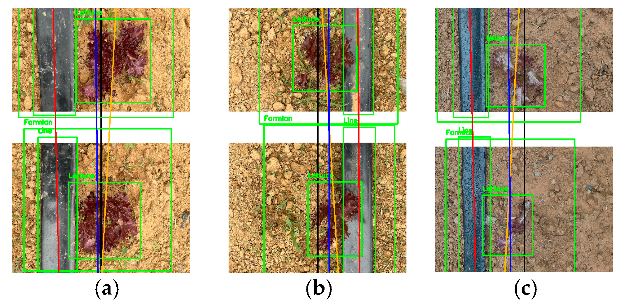
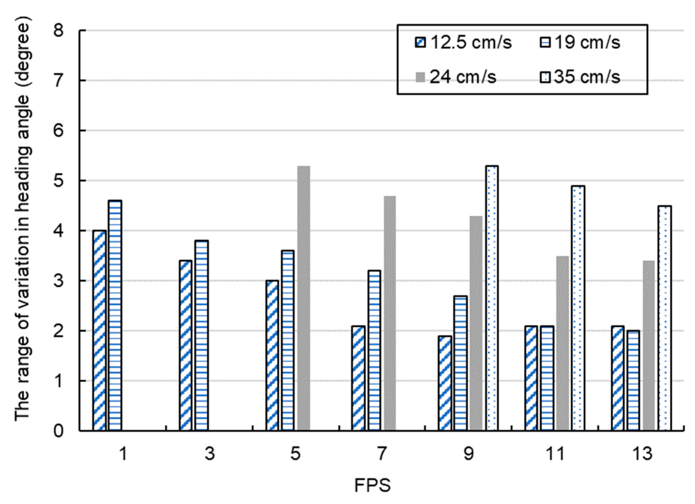
• The fitting result of the guidance line is related to the speed of the robot, the detection performance of DetModel #1, and the FPS value. As shown in Table 4, the accuracy of using DetModel #1 to detect ridges, crops, or drip irrigation belts ranged from 92 to 99%, with an average accuracy (AP) of about 95%. The accuracy of identifying drip irrigation belts was the highest, reaching up to 99%, followed by crops at 98% and field ridges at 97%. Since the training set samples came from images captured in a real environment from different angles and under various weather conditions, such realistic datasets can enhance the object recognition ability of the model [47,48]. The accuracy of navigation line extraction depends on the performance of the trained model in detecting targets. When the same type of object of the image is successfully detected multiple times, a line can be fitted using the least squares method. Soil images under different climate conditions were collected, and even overexposed images were used as training samples for modeling. The experimental results show that the trained model can effectively improve its generalization performance, especially under different climate conditions. In practical operation, as long as the center points of at least two objects can be detected, the navigation line can be extracted.
  When the robot traveled at a speed of 12.5 cm/s, and the FPS is set to 7, its mAP could reach 98%. As the robot speed increased, the mAP gradually decreased. When comparing the relationship between the mAP and heading angle variation in Figure 19 and Figure 21, it can be observed that a lower mAP would lead to an increased range of heading angle variation, producing more dubious heading angles. Increasing the FPS can help reduce false detection for objects caused by instantaneous strong ambient light and maintain a certain mAP even as the speed of robot increases. However, it also increases the computing load of the system, leading to the risk of overheating of the hardware system. Under conditions that meet various climatic requirements while maintaining the average object detection performance, the average detection time of DetModel #1 was 143 ms/per image.
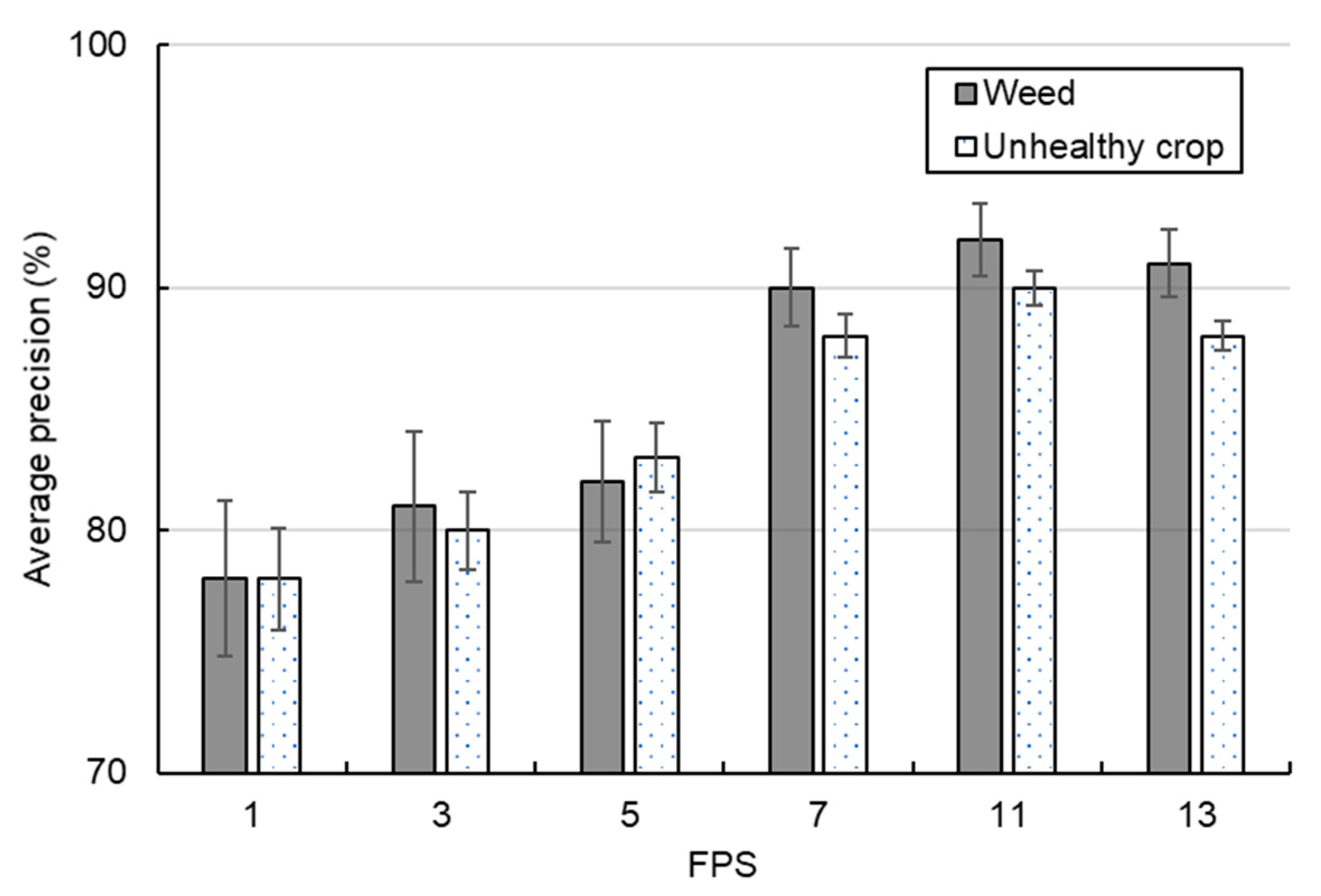
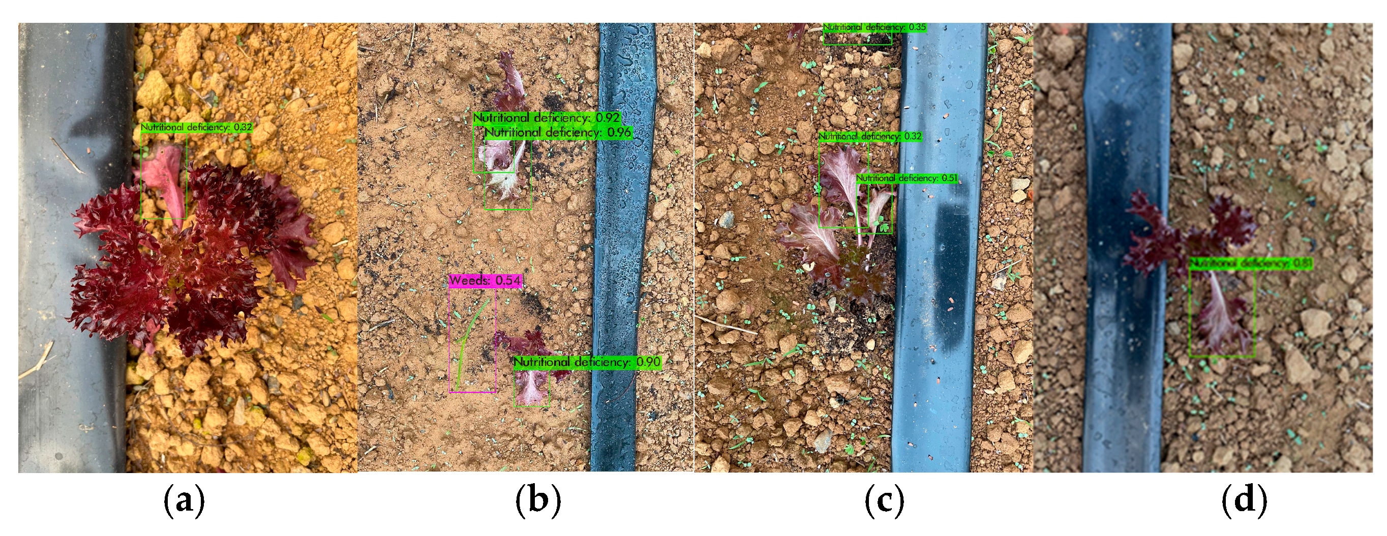
• Under different weather conditions, DetModel #2 was used to identify unhealthy crops and weeds, achieving average PRs of about 84% and 93%, respectively. In the afternoon on a cloudy day, the PR was slightly reduced to 84~89%, demonstrating that the deep learning model exhibited better adaptability to images with weaker light intensities. This adaptability improves upon the limitations of traditional machine learning techniques [49]. However, the limited dynamic illumination range of RGB cameras can easily lead to image color distortion when this limit is exceeded or not met [50], making object recognition difficult, especially with overexposed or insufficiently bright images.
  Rapid movement can result in specific frames failing to capture the target. Objects often have features significantly different from those encountered during the training process, making them difficult detect [25]. Changes in ambient lighting alter the tones and shadows in the image frame, affecting an object’s color, and pixel edge blur or shadows can also significantly impact detection accuracy [51,52]. Adding more feature information to the training of the deep learning model can improve its detection performance [53]. In this study, more field images, including soil types in low-light environments and even overexposed images, were used as samples. The experimental results show that the trained deep learning model had better generalization performance.
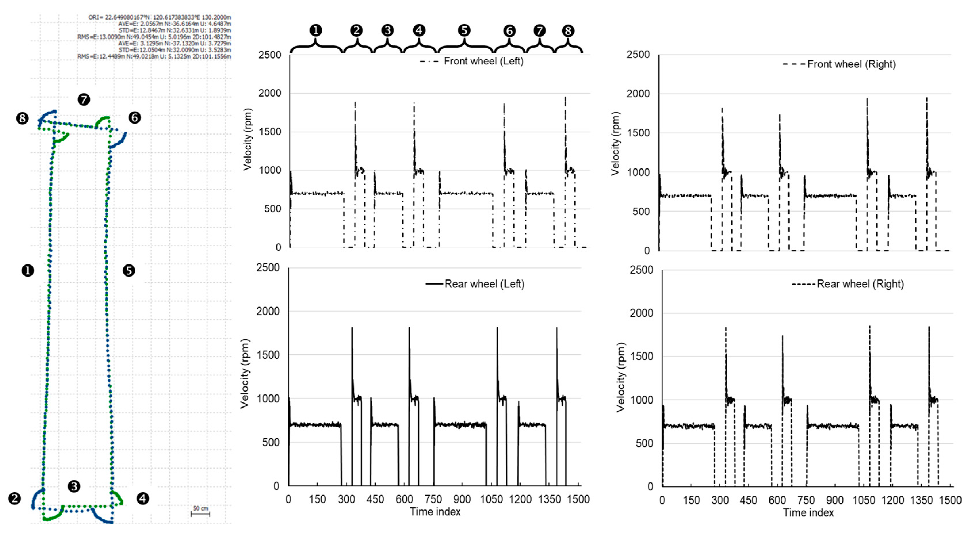
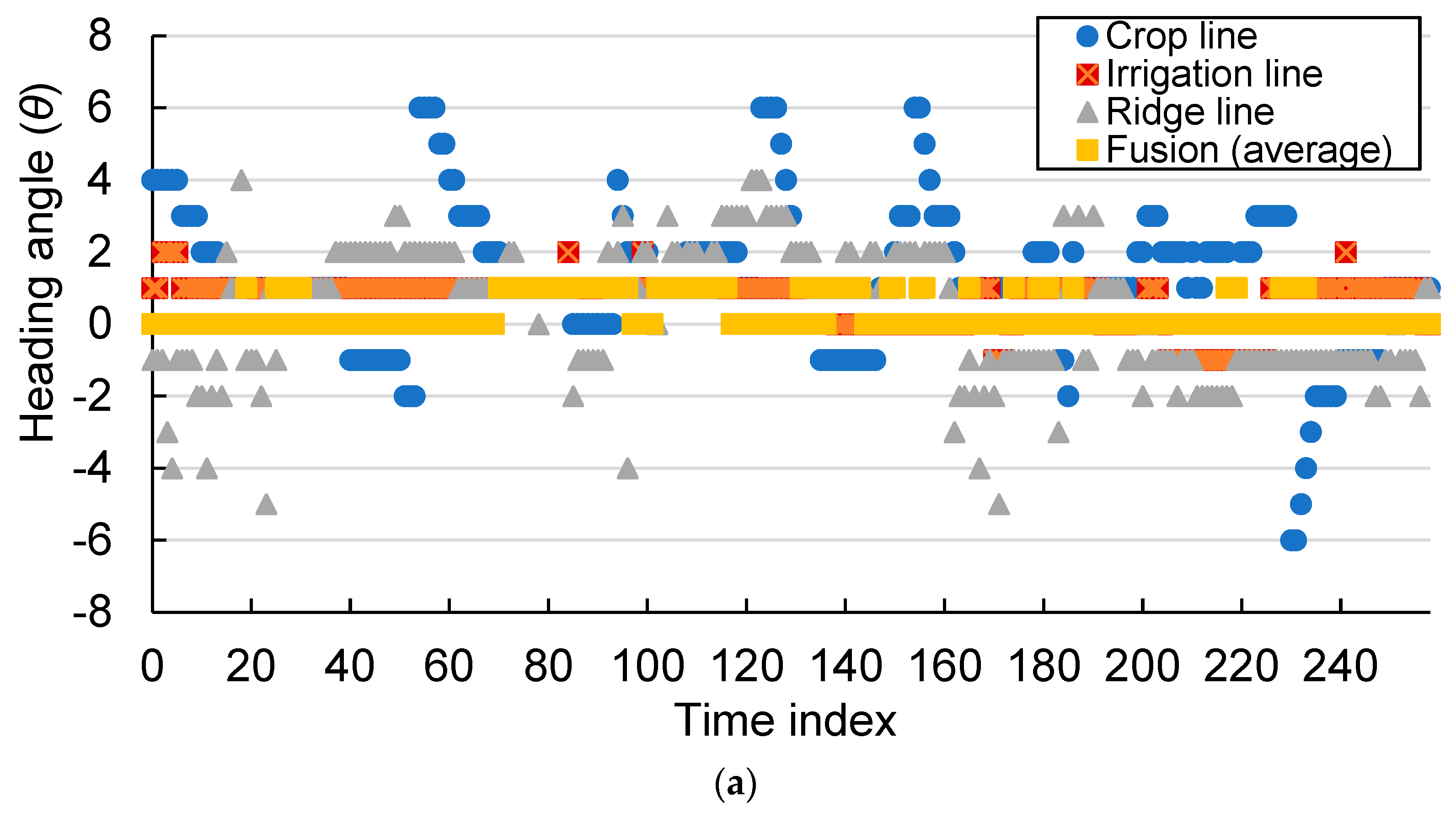
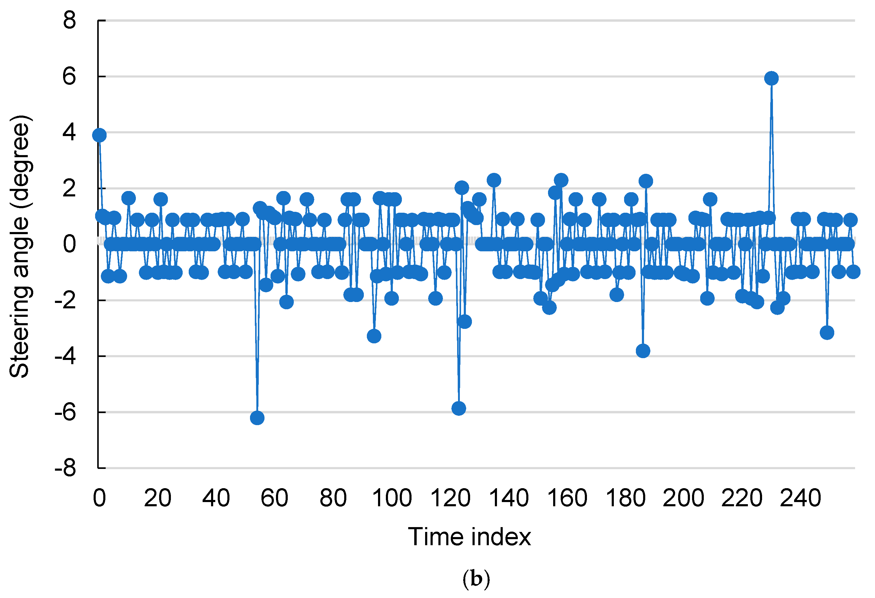
• Limited by the soil hardness and site flatness, in this study, the $K_p$ value of the PID controller was set to 0.5, enabling the four DC motors to reach the required speed quickly. Although there is a short-term small oscillation when the motor starts, its impact on the traveling speed of the robot is minimal. On the other hand, the FLC can smoothly adjust the heading angle and improve the two-wheel speed difference control method [54]. The experimental results show that when the robot moved in a guidance line at a speed of 12.5 cm/s, the variation in the heading angle stayed within one degree. Although no drip irrigation belt was present on the field, the average variation range of the heading angle remained within ±3.5 degrees (Figure 18a). Assuming that the planting position of the crops in the image was not on the vertical line in the center of the field ridge, it would also affect the estimated heading angle when the robot moved. For instance, in Figure 18a, at time indices of about 55, 130, 125, and 232, the heading angle estimated based on the crop line changed instantly by more than four degrees. Fortunately, this result has to be averaged with the heading angles obtained from the other regression lines, preventing ridge damage due to overcorrection of the wheels and avoiding misjudgment of the heading angle. When the robot rotated, a higher motor speed output value (1000 rpm) was used, ensuring greater torque was instantly available and allowing the four drives to power the motors. The advantage of the 4 WD/4 WS system is that it enables the robot to achieve a turning radius of zero. Compared with common car drive systems, this steering mode reduces the space required for turning and improves land use efficiency. Moreover, relying on RTK-GNSS receivers for centimeter-level autonomous guidance of a farming robot is a common practice [55]. This centimeter-level positioning error is acceptable when a fixed ambiguity solution is obtained [56]. However, there are risks in autonomous guiding operations on narrow farming areas. If the positioning signal is interrupted, or the positioning solution is a floating solution, then the robot may damage the field during movement.
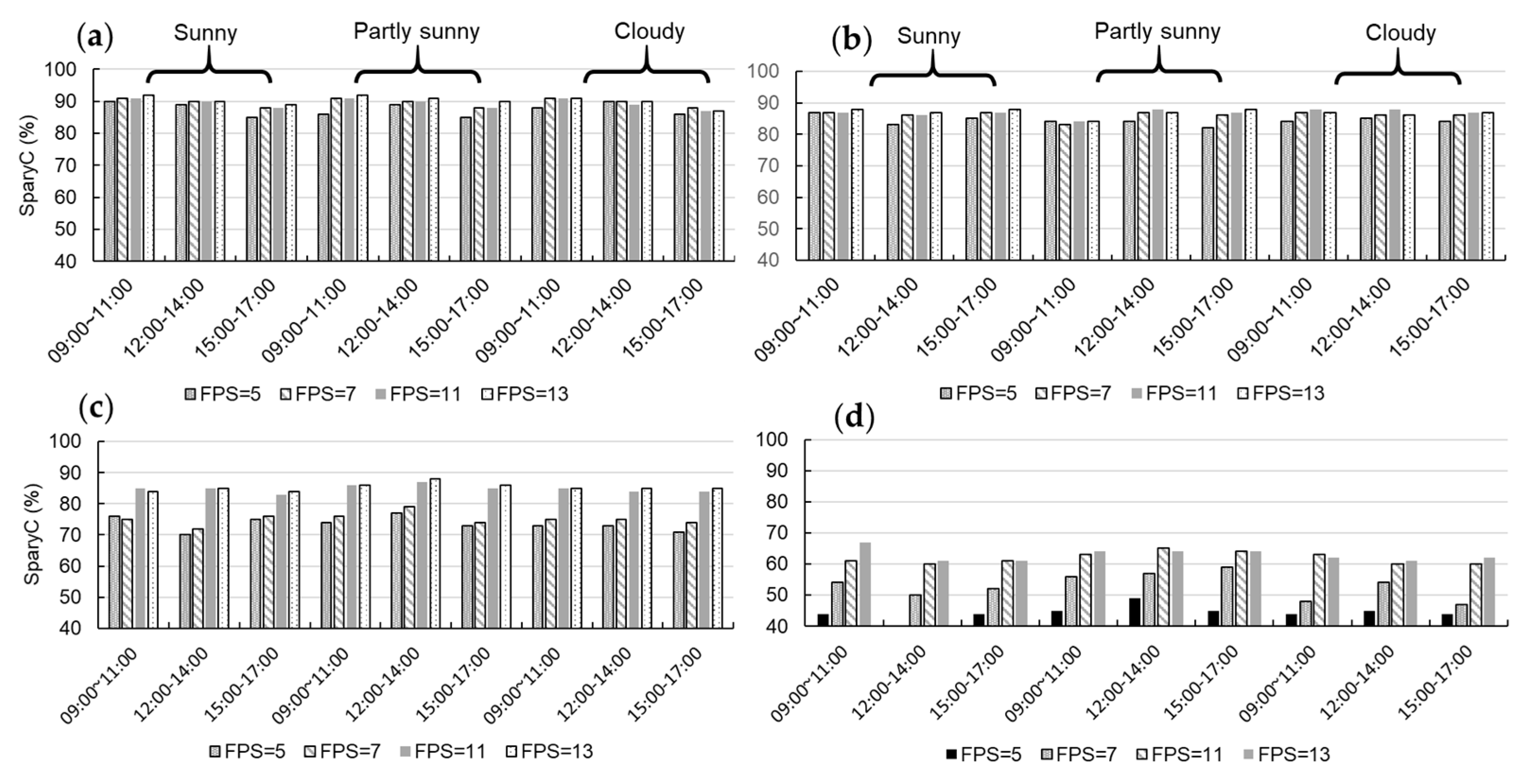
• During spraying test operation, setting the delay time of the sprayer according to the speed of the robot can avoid ineffective spraying. In this study, when the robot speed was 12.5 cm/s, with a sprayer time of about 0.5 s and a delay time of 2.5 s, the EWC and IWC reached 83% and 8% respectively, and the pesticide reduction reached 53%. Similar results were also presented in [57], with a 34.5% reduction in pesticide usage compared with traditional uniform spraying methods. As the speed of the robot increased, the EWC decreased, and the IWC increased. At a speed of 35 cm/s, the average precision was too low, which indirectly resulted in a reduction in the number of pesticide applications. On the other hand, the unhealthy crops were about 7–12 cm in diameter. Even with the appropriate delay time set, there were still some unhealthy crops or weeds that could not be sprayed correctly.

5. Conclusions

This study offers insights into the challenges and potential solutions for agricultural robots in real-world applications. Agricultural robots must rely on high-precision positioning systems to complete autonomous operations in the field. In practice, 4WS/4WD agricultural robots are utilized to navigate strip fields, turning on the spot to transition to other farming areas. Firstly, the experimental results confirmed that the deep learning model can detect drip irrigation belts, field ridges, crops, unhealthy crops, and weed objects with an accuracy rate ranging from 83 to 99%. This enables the implementation of various operations in climatically diverse environments, such as inter-row line tracking and selective spraying. In terms of robot guidance line tracking, this study presents an innovative method that estimates the robot’s heading angle using multiple regression lines. This method has been proven to be more reliable than conventional crop row extraction techniques, significantly reducing the risk of oversteering and potential damage to crops and field ridges during the robot’s movement. The deviation angle was within one degree at a speed of 12.5 cm/s, assisted by multiple guidance lines and using a PID controller and FLC. Minimizing human factors, such as misaligned crop planting and uneven crop spacing, will enhance the accuracy of the heading angle.

Secondly, an excessively fast robot movement speed causes the object detection rate to decrease. The reason involves limited computing resources leading to insufficient FPS values. By allowing the robot to operate at a slower speed, we ensure the maintenance of a certain level of object detection performance for selective spraying operations. At a frame processing rate of 7 FPS and a robot speed of 12.5 cm/s, the mAP for detecting weeds and unhealthy crops ranged from 93 to 98%. The accuracy of spraying unhealthy crops could reach up to 92%. Considering the sprayer’s fixed delay time, the autonomous robot achieved an effective weed coverage rate of 83% and a pesticide saving rate of 53% while operating at a speed of 12.5 cm/s. The applicability of these advancements to low-cost hardware expands their impact across various agricultural settings, particularly benefiting small-scale and resource-limited farming. Future research will concentrate on integrating adaptive FPS and minimizing spray start latency in autonomous agricultural robots, enabling them to perform a variety of tasks in a decentralized fashion.

References

- Spykman, O.; Gabriel, A.; Ptacek, M.; Gandorfer, M. Farmers’ perspectives on field crop robots—Evidence from Bavaria, Germany. Comput. Electron. Agric. 2021, 186, 106176. [Google Scholar] [CrossRef]
- Wu, J.; Jin, Z.; Liu, A.; Yu, L.; Yang, F. A survey of learning-based control of robotic visual servoing systems. J. Franklin Inst. 2022, 359, 556–577. [Google Scholar] [CrossRef]
- Kato, Y.; Morioka, K. Autonomous robot navigation system without grid maps based on double deep Q-Network and RTK-GNSS localization in outdoor environments. In Proceedings of the 2019 IEEE/SICE International Symposium on System Integration (SII), Paris, France, 14–16 January 2019; pp. 346–351. [Google Scholar]
- Galati, R.; Mantriota, G.; Reina, G. RoboNav: An affordable yet highly accurate navigation system for autonomous agricultural robots. Robotics 2022, 11, 99. [Google Scholar] [CrossRef]
- Chien, J.C.; Chang, C.L.; Yu, C.C. Automated guided robot with backstepping sliding mode control and its path planning in strip farming. Int. J. iRobotics 2022, 5, 16–23. [Google Scholar]
- Zhang, L.; Zhang, R.; Li, L.; Ding, C.; Zhang, D.; Chen, L. Research on virtual Ackerman steering model based navigation system for tracked vehicles. Comput. Electron. Agric. 2022, 192, 106615. [Google Scholar] [CrossRef]
- Tian, H.; Wang, T.; Liu, Y.; Qiao, X.; Li, Y. Computer vision technology in agricultural automation—A review. Inf. Process. Agric. 2020, 7, 1–19. [Google Scholar] [CrossRef]
- Leemans, V.; Destain, M.F. Application of the Hough transform for seed row localisation using machine vision. Biosyst. Eng. 2006, 94, 325–336. [Google Scholar] [CrossRef]
- Choi, K.H.; Han, S.K.; Han, S.H.; Park, K.-H.; Kim, K.-S.; Kim, S. Morphology-based guidance line extraction for an autonomous weeding robot in paddy fields. Comput. Electron. Agric. 2015, 113, 266–274. [Google Scholar] [CrossRef]
- Zhou, X.; Zhang, X.; Zhao, R.; Chen, Y.; Liu, X. Navigation line extraction method for broad-leaved plants in the multi-period environments of the high-ridge cultivation mode. Agriculture 2023, 13, 1496. [Google Scholar] [CrossRef]
- Suriyakoon, S.; Ruangpayoongsak, N. Leading point-based interrow robot guidance in corn fields. In Proceedings of the 2017 2nd International Conference on Control and Robotics Engineering (ICCRE), Bangkok, Thailand, 1–3 April 2017; pp. 8–12. [Google Scholar]
- Bonadiesa, S.; Gadsden, S.A. An overview of autonomous crop row navigation strategies for unmanned ground vehicles. Eng. Agric. Environ. Food 2019, 12, 24–31. [Google Scholar] [CrossRef]
- Chen, J.; Qiang, H.; Wu, J.; Xu, G.; Wang, Z. Navigation path extraction for greenhouse cucumber-picking robots using the prediction-point Hough transform. Comput. Electron. Agric. 2021, 180, 105911. [Google Scholar] [CrossRef]
- Ma, Z.; Tao, Z.; Du, X.; Yu, Y.; Wu, C. Automatic detection of crop root rows in paddy fields based on straight-line clustering algorithm and supervised learning method. Biosyst. Eng. 2021, 211, 63–76. [Google Scholar] [CrossRef]
- Shi, J.; Bai, Y.; Diao, Z.; Zhou, J.; Yao, X.; Zhang, B. Row detection-based navigation and guidance for agricultural robots and autonomous vehicles in row-crop fields: Methods and applications. Agronomy 2023, 13, 1780. [Google Scholar] [CrossRef]
- Zhang, S.; Wang, Y.; Zhu, Z.; Li, Z.; Du, Y.; Mao, E. Tractor path tracking control based on binocular vision. Inf. Process. Agric. 2018, 5, 422–432. [Google Scholar] [CrossRef]
- Mavridou, E.; Vrochidou, E.; Papakostas, G.A.; Pachidis, T.; Kaburlasos, V.G. Machine vision systems in precision agriculture for crop farming. J. Imaging 2019, 5, 89. [Google Scholar] [CrossRef]
- Gu, Y.; Li, Z.; Zhang, Z.; Li, J.; Chen, L. Path tracking control of field information-collecting robot based on improved convolutional neural network algorithm. Sensors 2020, 20, 797. [Google Scholar] [CrossRef]
- Pajares, G.; García-Santillán, I.; Campos, Y.; Montalvo, M.; Guerrero, J.M.; Emmi, L.; Romeo, J.; Guijarro, M.; González-de-Santos, P. Machine-vision systems selection for agricultural vehicles: A guide. J. Imaging 2016, 2, 34. [Google Scholar] [CrossRef]
- de Silva, R.; Cielniak, G.; Gao, J. Towards agricultural autonomy: Crop row detection under varying field conditions using deep learning. arXiv 2021, arXiv:2109.08247. [Google Scholar]
- Hu, Y.; Huang, H. Extraction method for centerlines of crop row based on improved lightweight Yolov4. In Proceedings of the 2021 6th International Symposium on Computer and Information Processing Technology (ISCIPT), Changsha, China, 11–13 June 2021; pp. 127–132. [Google Scholar]
- Ruan, Z.; Chang, P.; Cui, S.; Luo, J.; Gao, R.; Su, Z. A precise crop row detection algorithm in complex farmland for unmanned agricultural machines. Biosyst. Eng. 2023, 232, 1–12. [Google Scholar] [CrossRef]
- Ruigrok, T.; van Henten, E.; Booij, J.; van Boheemen, K.; Kootstra, G. Application-specific evaluation of a weed-detection algorithm for plant-specific spraying. Sensors 2020, 20, 7262. [Google Scholar] [CrossRef]
- Hu, D.; Ma, C.; Tian, Z.; Shen, G.; Li, L. Rice Weed detection method on YOLOv4 convolutional neural network. In Proceedings of the 2021 International Conference on Artificial Intelligence, Big Data and Algorithms (CAIBDA), Xi’an, China, 28–30 May 2021; pp. 41–45. [Google Scholar]
- Chang, C.L.; Xie, B.X.; Chung, S.C. Mechanical control with a deep learning method for precise weeding on a farm. Agriculture 2021, 11, 1049. [Google Scholar] [CrossRef]
- Wang, Q.; Cheng, M.; Huang, S.; Cai, Z.; Zhang, J.; Yuan, H. A deep learning approach incorporating YOLO v5 and attention mechanisms for field real-time detection of the invasive weed Solanum rostratum Dunal seedlings. Comput. Electron. Agric. 2022, 199, 107194. [Google Scholar] [CrossRef]
- Chen, J.; Wang, H.; Zhang, H.; Luo, T.; Wei, D.; Long, T.; Wang, Z. Weed detection in sesame fields using a YOLO model with an enhanced attention mechanism and feature fusion. Comput. Electron. Agric. 2022, 202, 107412. [Google Scholar] [CrossRef]
- Ruigrok, T.; van Henten, E.J.; Kootstra, G. Improved generalization of a plant-detection model for precision weed control. Comput. Electron. Agric. 2023, 204, 107554. [Google Scholar] [CrossRef]
- Razfar, N.; True, J.; Bassiouny, R.; Venkatesh, V.; Kashef, R. Weed detection in soybean crops using custom lightweight deep learning models. J. Agric. Food Res. 2022, 8, 100308. [Google Scholar] [CrossRef]
- Qiu, Q.; Fan, Z.; Meng, Z.; Zhang, Q.; Cong, Y.; Li, B.; Wang, N.; Zhao, C. Extended Ackerman steering principle for the co-ordinated movement control of a four wheel drive agricultural mobile robot. Comput. Electron. Agric. 2018, 152, 40–50. [Google Scholar] [CrossRef]
- Bak, T.; Jakobsen, H. Agricultural robotic platform with four wheel steering for weed detection. Biosyst. Eng. 2004, 87, 125–136. [Google Scholar] [CrossRef]
- Tu, X.; Gai, J.; Tang, L. Robust navigation control of a 4WD/4WS agricultural robotic vehicle. Comput. Electron. Agric. 2019, 164, 104892. [Google Scholar] [CrossRef]
- Wang, D.; Qi, F. Trajectory planning for a four-wheel-steering vehicle. In Proceedings of the 2001 ICRA. IEEE International Conference on Robotics and Automation, Seoul, Republic of Korea, 21–26 May 2001; Volume 4, pp. 3320–3325. [Google Scholar]
- Bochkovskiy, A.; Wang, C.-Y.; Liao, H.M. YOLOv4: Optimal speed and accuracy of object detection. arXiv 2020, arXiv:2004.10934. [Google Scholar]
- Redmon, J.; Farhadi, A. YOLOv3: An incremental improvement. arXiv 2018, arXiv:1804.02767. [Google Scholar]
- Wang, C.Y.; Liao, H.Y.M.; Wu, Y.H.; Chen, P.Y.; Hsieh, J.W.; Yeh, I.H. CSPNet: A new backbone that can enhance learning capability of CNN. In Proceedings of the 2020 IEEE/CVF Conference on Computer Vision and Pattern Recognition Work-shops (CVPRW), Seattle, WA, USA, 14–19 June 2020; pp. 1571–1580. [Google Scholar]
- He, K.; Zhang, X.; Ren, S.; Sun, J. Spatial pyramid pooling in deep convolutional networks for visual recognition. IEEE Trans. Pattern Anal. Mach. Intell. 2015, 37, 1904–1916. [Google Scholar] [CrossRef] [PubMed]
- Zhang, Z.; He, T.; Zhang, H.; Zhang, Z.; Xie, J.; Li, M. Bag of freebies for training object detection neural networks. arXiv 2019, arXiv:1902.04103. [Google Scholar]
- Zheng, Z.; Wang, P.; Liu, W.; Li, J.; Ye, R.; Ren, D. Distance-IoU loss: Faster and better learning for bounding box regression. AAAI Tech. Track Vis. 2020, 34, 12993–13000. [Google Scholar] [CrossRef]
- Roy, A.M.; Bhaduri, J. Real-time growth stage detection model for high degree of occultation using DenseNet-fused YOLOv4. Comput. Electron. Agric. 2022, 193, 106694. [Google Scholar] [CrossRef]
- Chang, C.L.; Chen, H.W. Straight-line generation approach using deep learning for mobile robot guidance in lettuce fields. In Proceedings of the 2023 9th International Conference on Applied System Innovation (ICASI), Chiba, Japan, 21–25 April 2023. [Google Scholar]
- Lee, C.C. Fuzzy logic in control system: Fuzzy logic controller. IEEE Trans. Syst. Man Cybern. Syst. 1990, 20, 404–418. [Google Scholar] [CrossRef]
- Yu, C.C.; Tsen, Y.W.; Chang, C.L. Modeled Carrier. TW Patent No. I706715, 11 October 2020. [Google Scholar]
- Bennett, P. The NMEA FAQ (Fragen und Antworten zu NMEA), Ver. 6.1; Sepember 1997. Available online: https://www.geocities.ws/lrfernandes/gps_project/Appendix_E_NMEA_FAQ.pdf (accessed on 30 January 2023).
- Shih, P.T.-Y. TWD97 and WGS84, datum or map projection? J. Cadastr. Surv. 2020, 39, 1–12. [Google Scholar]
- Lee, J.; Hwang, K.I. YOLO with adaptive frame control for real-time object detection applications. Multimed. Tools Appl. 2022, 81, 36375–36396. [Google Scholar] [CrossRef]
- Hasan, R.I.; Yusuf, S.M.; Alzubaidi, L. Review of the state of the art of deep learning for plant diseases: A broad analysis and discussion. Plants 2020, 9, 1302. [Google Scholar] [CrossRef]
- Arsenovic, M.; Karanovic, M.; Sladojevic, S.; Anderla, A.; Stefanovic, D. Solving current limitations of deep learning based approaches for plant disease detection. Symmetry 2019, 11, 939. [Google Scholar] [CrossRef]
- Zhang, Y.; Chen, H.; He, Y.; Ye, M.; Cai, X.; Zhang, D. Road segmentation for all-day outdoor robot navigation. Neurocomputing 2018, 314, 316–325. [Google Scholar] [CrossRef]
- Liu, J.; Wang, X. Plant diseases and pests detection based on deep learning: A review. Plant Methods 2021, 17, 22–35. [Google Scholar] [CrossRef] [PubMed]
- Jiao, L.; Zhang, R.; Liu, F.; Yang, S.; Hou, B.; Li, L.; Tang, X. New generation deep learning for video object detection: A survey. IEEE Trans. Neural Netw. Learn. Syst. 2021, 33, 3195–3215. [Google Scholar] [CrossRef] [PubMed]
- Li, D.; Wang, R.; Xie, C.; Liu, L.; Zhang, J.; Li, R.; Wang, F.; Zhou, M.; Liu, W. A recognition method for rice plant diseases and pests video detection based on deep convolutional neural network. Sensors 2020, 20, 578. [Google Scholar] [CrossRef]
- Altalak, M.; Ammad uddin, M.; Alajmi, A.; Rizg, A. Smart agriculture applications using deep learning technologies: A survey. Appl. Sci. 2022, 12, 5919. [Google Scholar] [CrossRef]
- Chang, C.L.; Chen, H.W.; Chen, Y.H.; Yu, C.C. Drip-tape-following approach based on machine vision for a two-wheeled robot trailer in strip farming. Agriculture 2022, 12, 428. [Google Scholar] [CrossRef]
- del Rey, J.C.; Vega, J.A.; Pérez-Ruiz, M.; Emmi, L. Comparison of positional accuracy between RTK and RTX GNSS based on the autonomous agricultural vehicles under field conditions. Appl. Eng. Agric. 2014, 30, 361–366. [Google Scholar]
- Han, J.H.; Park, C.H.; Park, Y.J.; Kwon, J.H. Preliminary results of the development of a single-frequency GNSS RTK-based autonomous driving system for a speed sprayer. J. Sens. 2019, 2019, 4687819. [Google Scholar] [CrossRef]
- Gonzalez-de-Soto, M.; Emmi, L.; Perez-Ruiz, M.; Aguera, J.; Gonzalez-de-Santos, P. Autonomous systems for precise spraying—Evaluation of a robotised patch sprayer. Biosyst. Eng. 2016, 146, 165–182. [Google Scholar] [CrossRef]