Fault Diagnosis for Rolling Bearing Based on Semi-Supervised Clustering and Support Vector Data Description with Adaptive Parameter Optimization and Improved Decision Strategy

Abstract

Rolling bearing is of great importance in modern industrial products, the failure of which may result in accidents and economic losses. Therefore, fault diagnosis of rolling bearing is significant and necessary and can enhance the reliability and efficiency of mechanical systems. Therefore, a novel fault diagnosis method for rolling bearing based on semi-supervised clustering and support vector data description (SVDD) with adaptive parameter optimization and improved decision strategy is proposed in this study. First, variational mode decomposition (VMD) was applied to decompose the vibration signals into sets of intrinsic mode functions (IMFs), where the decomposing mode number K was determined by the central frequency observation method. Next, fuzzy entropy (FuzzyEn) values of all IMFs were calculated to construct the feature vectors of different types of faults. Later, training samples were clustered with semi-supervised fuzzy C-means clustering (SSFCM) for fully exploiting the information inside samples, whereupon a small number of labeled samples were able to provide sufficient data distribution information for subsequent SVDD algorithms and improve its recognition ability. Afterwards, SVDD with improved decision strategy (ID-SVDD) that combined with k-nearest neighbor was proposed to establish diagnostic model. Simultaneously, the optimal parameters C and σ for ID-SVDD were searched by the newly proposed sine cosine algorithm improved with adaptive updating strategy (ASCA). Finally, the proposed diagnosis method was applied for engineering application as well as contrastive analysis. The obtained results reveal that the proposed method exhibits the best performance in all evaluation metrics and has advantages over other comparison methods in both precision and stability.

1. Introduction

Rolling bearing is one of the most commonly used components in mechanical equipment, whose running state directly affects the accuracy, reliability, and service life of the whole machine [1]. Hence, how to recognize and diagnose rolling bearing faults remains one of the main concerns in preventing failures of mechanical systems [2]. However, rolling bearing is prone to failure due to the complex operating conditions, such as improper assembly, poor lubrication, water and foreign body invasion, corrosion or overload [3]. Therefore, effective methods need to be proposed to diagnosis a fault of rolling bearing, which can promote the reliability of industrial manufacture.

Owing to the rich information carried by vibration signals, most of fault diagnosis methods for rolling bearings rely on analyzing vibration signals [4,5], the resistance of the bearing can be measured using electrodynamic sensors or laser vibrometers [6]. Considering that vibration signals are commonly non-stationary, it is difficult to extract critical features directly from fault signals. To solve this problem, various non-stationary signal processing methods are proposed in previous studies. For instance, wavelet transform (WT) is a self-adaptive signal decomposition method [7], which inherits and develops the idea of localization of short-time Fourier transform and is an ideal tool for time-frequency analysis, but its generalization will be restricted once a wavelet basis is chosen. Empirical mode decomposition (EMD) has a strong ability to deal with non-stationary signals and does not need to pre-set any basis function [8], but its performance is affected by end effects and mode mixing. To overcome these defects, an improved version of EMD, ensemble empirical mode decomposition (EEMD), is proposed by introducing a noise-assisted analysis method [9], which is also increases the computational cost and cannot completely neutralize the added noise. Unlike the above methods, variational mode decomposition (VMD) is a novel quasi-orthogonal signal decomposition method which overcomes the generalization problem of WT or mode mixing and end effects of EMD and EEMD [10]. Its advancement and effectiveness have been demonstrated in previous studies [11,12]. With signals processed by non-stationary analytical method, the non-stationarity of signals would be weakened to some extent, and fault features can be further extracted. Due to the smoothness and robustness, as well as fewer samples required, fuzzy entropy (FuzzyEn) [13] is introduced to measure the features of vibration data and construct fault samples, which has been widely applied for feature extraction and shows superior performance in the field of fault diagnosis [14,15].

Fault diagnosis of rolling bearings is actually a problem of pattern recognition [16], and many machine learning methods have been developed for this problem [17]. Traditional machine learning methods require a large amount of labeled data to ensure the generalization of the algorithm. However, in practical problems, most of the samples are unlabeled, which results in unsatisfactory results of trained learning models in practical applications and makes a large number of unlabeled samples useless. Hence, semi-supervised methods are applied to fully exploit the information inside samples and expand the training set of machine learning algorithms. Semi-supervised fuzzy C-means clustering (SSFCM) [18] is a “semi-supervised version” of the fuzzy C-means clustering (FCM) algorithm. By introducing semi-supervised learning theory into FCM, training samples can be labeled under the supervision of the partly labeled samples, which makes up for the deficiency of labeled samples and improving the accuracy of pattern recognition [19,20]. In engineering application, several machine learning methods, including k-nearest neighbor (KNN) [21], artificial neural network (ANN) [22], support vector machine (SVM) [23] and support vector data description (SVDD) [24] are widely applied to solve pattern recognition problems. KNN is easy to realize and susceptible to the distribution of samples. ANN has good performance in dealing with non-linear problems under the circumstance of a large number of samples. Based on structural risk minimization and statistical learning theory, SVM proposed by Vapnik finds an optimal hyperplane that meets the classification requirements, thus the hyperplane maximizes the interval between two classes while ensuring classification effect. Correspondingly, SVDD is a kernel method inspired by the idea of SVM theory [25], which possesses a prominent recognition ability through establishing a minimum hypersphere that contains as many samples as possible [26]. Currently, combined with relative distance decision strategy, SVDD has been successfully employed in the field of pattern recognition [27,28]. However, traditional relative distance decision strategy is difficult to accurately classify unknown samples locating in overlap regions of the hyperspheres and regions outside all the hyperspheres. To solve this problem, SVDD based on an improved decision strategy (ID-SVDD) with the fusion of KNN method is proposed. To be specific, support vectors (SVs) are firstly extracted by establishing SVDD models. Next, the Euclidean distances between the testing sample and SVs are calculated. Whereupon, a fault type of the testing sample can be determined according to the proposed decision strategy.

Although SVDD has excellent effect in pattern recognition, its performance is affected by the parameters. In view of this, various optimization algorithms are proposed and applied to search the best parameters [29,30], including genetic algorithm (GA) [31], particle swarm optimization (PSO) [32], bacterial foraging algorithm (BFA) [33] and artificial sheep algorithm (ASA) [34]. As a novel optimization algorithm, sine cosine algorithm (SCA) proposed by Mirjalili [35] is proved to be effective in many studies [36,37]. To achieve better performance in convergence precision, a reformed sine cosine algorithm with adaptive strategy (ASCA) is developed in this paper. On the whole, a novel diagnosis method based on semi-supervised clustering and SVDD with adaptive parameter optimization and improved decision strategy is proposed in this study. Firstly, VMD is applied to decompose the vibration signals into sets of IMFs, and the decomposing mode number K is preset with central frequency observation method. Then FuzzyEn values of all IMFs are calculated to construct the feature vectors of corresponding samples with different fault types. Afterwards, training samples are clustered by SSFCM for information mining. Subsequently, SVDD with improved decision strategy (ID-SVDD) that combines with k-nearest neighbor is proposed to establish diagnostic model. Meanwhile, the optimal parameters C and σ for ID-SVDD is searched by the proposed adaptive sine cosine algorithm (ASCA). Finally, the engineering application and contrastive analysis indicate the availability and superiority of the proposed method.

The paper is organized as follows: Section 2 is dedicated to the basic knowledge of VMD, FuzzyEn, SSFCM, and SVDD. Section 3 introduces the proposed fault diagnosis method based on SSFCM and ASCA-optimized ID-SVDD. Section 4 presents the engineering application and comparative analysis, the experimental results of which demonstrate the superiority of the proposed method. Some discussion about the method presented in this paper is in Section 5. The conclusion is summarized in Section 6.

2. Fundamental Theories

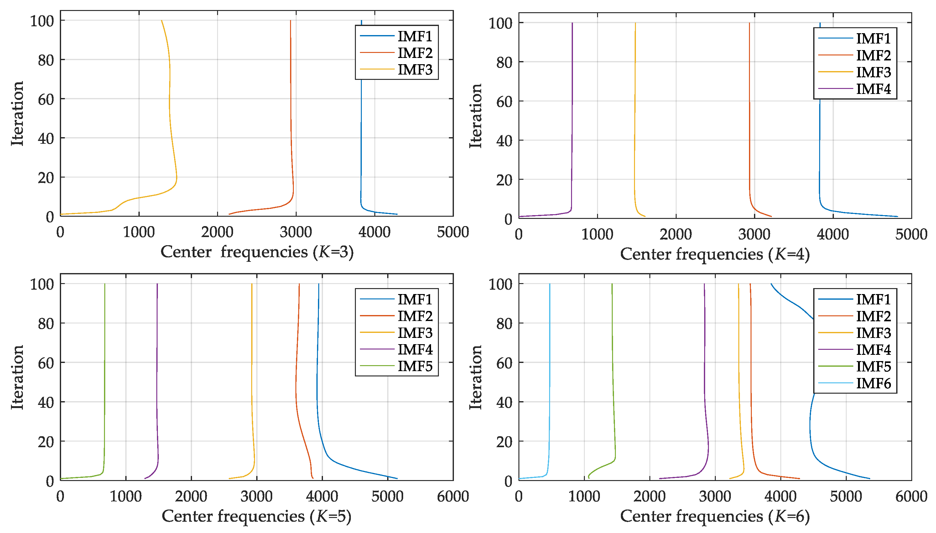
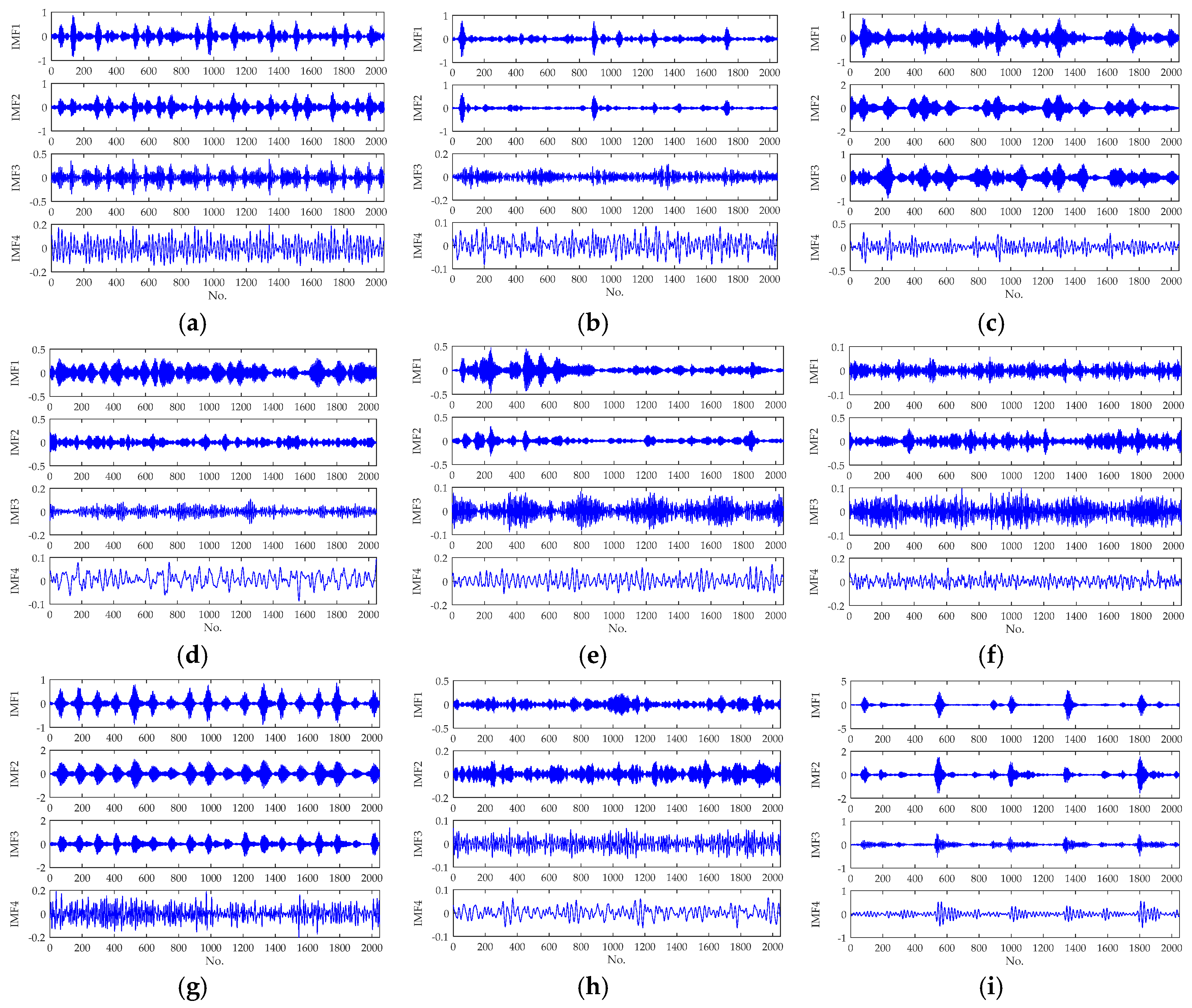
2.1. Variational Mode Decomposition

Variational mode decomposition (VMD) is a novel non-recursive signal decomposition method [38], whose essence is to solve a variational optimization problem. Setting a scale K in advance, a given signal can be decomposed into K band-limited intrinsic mode functions (IMFs), among which each sub-signal is related to a certain center frequency. The constrained variation problem can be described as follows:

$$\begin{array}{l}\underset{m_k,{\omega }_k}{\min }\{{\displaystyle \sum _{k=1}^K{\Vert {\partial }_t\left[\left(\delta (t)+\frac{j}{\pi t}\right)\ast m_k(t)\right]e^{-j{\omega }_{k}t}\Vert }_2^2}\}\\ s.t.\hspace{0.17em}\hspace{0.17em}\hspace{0.17em}{\displaystyle \sum _{k=1}^K{m}_k}=f,\hspace{0.17em}\hspace{0.17em}\hspace{0.17em}k=1,2,\dots ,K\end{array}$$

(1)

where $m_k=\{m_1,m_2,\dots ,m_k\}$ represents the set of all mode functions, and ${\omega }_k=\{{\omega }_1,{\omega }_2,\dots ,{\omega }_k\}$ represents the set of center frequencies, while ${\partial }_t$ and $\delta (t)$ are the partial derivative of time t for the function and unit pulse function, respectively. f is the given real valued input signal.

Lagrange multipliers are introduced to obtain the optimal solution of above constrained variational problem. Then problem (1) can be specified as follows:

$$\begin{array}{ll}L(m_k,{\omega }_k,\beta )& =\alpha {\displaystyle \sum _{k=1}^K{\Vert {\partial }_t\left[\left(\delta (t)+\frac{j}{\pi t}\right)\ast m_k(t)\right]e^{-j{\omega }_{k}t}\Vert }_2^2}\\ & +\hspace{0.17em}{\Vert f(t)-{\displaystyle \sum _k^K{m}_k(t)}\Vert }_2^2+\langle \beta (t),f(t)-{\displaystyle \sum _k^K{m}_k(t)}\rangle \end{array}$$

(2)

where α and β(t) represent the penalty factor and Lagrange multiplier respectively.

Next, the alternate direction method of multipliers (ADMM) and iterative search are utilized to obtain the saddle point of Lagrange multipliers [39]. The optimization problems of m_k and 𝜔_k are formulated as (3) and (4) respectively.

$$m_k^{n+1}=\min \left\{\begin{array}{l}\alpha {\Vert {\partial }_t\left[\left(\delta (t)+\frac{j}{\pi t}\right)\ast m_k(t)\right]e^{-j{\omega }_{k}t}\Vert }_2^2\\ +{\Vert f(t)-{\displaystyle \sum _i{m}_i(t)+\frac{\beta (t)}{2}}\Vert }_2^2\end{array}\right\}$$

(3)

$${\omega }_k^{n+1}=\min \left\{{\Vert {\partial }_t\left[\left(\delta (t)+\frac{j}{\pi t}\right)\ast m_k(t)\right]e^{-j{\omega }_{k}t}\Vert }_2^2\right\}$$

(4)

Solving problems (3) and (4), the iterative equations are deduced as follows:

$${\widehat{m}}_k^{n+1}(\omega )=\frac{\widehat{f}(\omega )-{\displaystyle {\sum }_{i\ne k}{\widehat{m}}_i(\omega )+\frac{\widehat{\beta }(\omega )}{2}}}{1+2\alpha {(\omega -{\omega }_k)}^2}$$

(5)

$${\omega }_k^{n+1}=\frac{{\displaystyle {\int }_0^{\infty }\omega {\left|{\widehat{m}}_k(\omega )\right|}^{2}d\omega }}{{\displaystyle {\int }_0^{\infty }{\left|{\widehat{m}}_k(\omega )\right|}^{2}d\omega }}$$

(6)

The Lagrange multipliers can be iterated with Equation (7).

$${\widehat{\beta }}^{n+1}(\omega )={\widehat{\beta }}^n(\omega )+\tau (f(\omega )-{\displaystyle \sum _k{\widehat{m}}_k^{n+1}(\omega ))}$$

(7)

where τ is an updating parameter.

The main steps of VMD can be summarized as follows:

Step 1: Initialize $m_k^1$, ${\omega }_k^1$, ${\beta }^1$, n = 1;

Step 2: Execute loop, n = n + 1;

Step 3: Update m_k and 𝜔_k based on Equations (5) and (6);

Step 4: Update β based on Equation (7);

Step 5: If ${\displaystyle \sum _k{\Vert {\widehat{m}}_k^{n+1}-{\widehat{m}}_k^n\Vert }_2^2}/{\Vert {\widehat{m}}_k^n\Vert }_2^2<\epsilon$ loop end, else turn to step 2 for next iteration.

2.2. Fuzzy Entropy

To solve the defect that sample entropy [40] adopts a hard threshold criterion which may result in an unstable discrimination result, fuzzy entropy [41] introduces an exponential function from fuzzy theory as the fuzzy entropy function. For the time series H = [h(1), h(2), ..., h(N)], set the fractal dimension m and then construct m-dimensional vector. The obtained m-dimensional vector is as follows:

$$H_m(i)=[h(i),h(i+1),\dots ,h(i+m-1)]-g(i)$$

(8)

where i = 1, 2, …, N − m + 1, and $g\left(i\right)=\frac{1}{m}{\displaystyle \sum _{j=0}^{m-1}h(i+j)}$.

Define the distance d_ij between vector H_m(i) and H_m(j) as maximum absolute value of difference value between the corresponding element of them, that is:

$$d_{ij}^m=\max |h(i+k)-g(i)-[h(j+k)-g(j)]|$$

(9)

where i, j = 1, 2, …, N − m + 1 and i ≠ j; while k = 0, 1, …, m − 1.

Introducing fuzzy membership function, the similarity between vector H_m(i) and H_m(j) can be defined as:

$$A_{ij}^m=\left\{\begin{array}{ll}1,& d_{ij}^m=0\\ \exp [-ln2{(\frac{d_{ij}^m}{r})}^2],& d_{ij}^m>0\end{array}\right\}$$

(10)

where r is a positive real number, and r = R·std(H), std(H) is the standard deviation of the given time series.

Define function ${\mathsf{\Phi }}^m(r)$ as:

$${\mathsf{\Phi }}^m(r)=\frac{1}{N-m+1}{\displaystyle \sum _{i=1}^{N-m+1}{C}_i^m}$$

(11)

where $C_i^m(r)=\frac{1}{N-m}{\displaystyle \sum _{j=1,j\ne i}^{N-m+1}{A}_{ij}^m}$.

Finally, FuzzyEn (with parameters m, N, r) of the time series can be deduced as the deviation of natural logarithm of ${\mathsf{\Phi }}^m$ from ${\mathsf{\Phi }}^{m+1}$, which means:

$$FE(m,N,r)=\ln {\mathsf{\Phi }}^m(r)-\ln {\mathsf{\Phi }}^{m+1}(r)$$

(12)

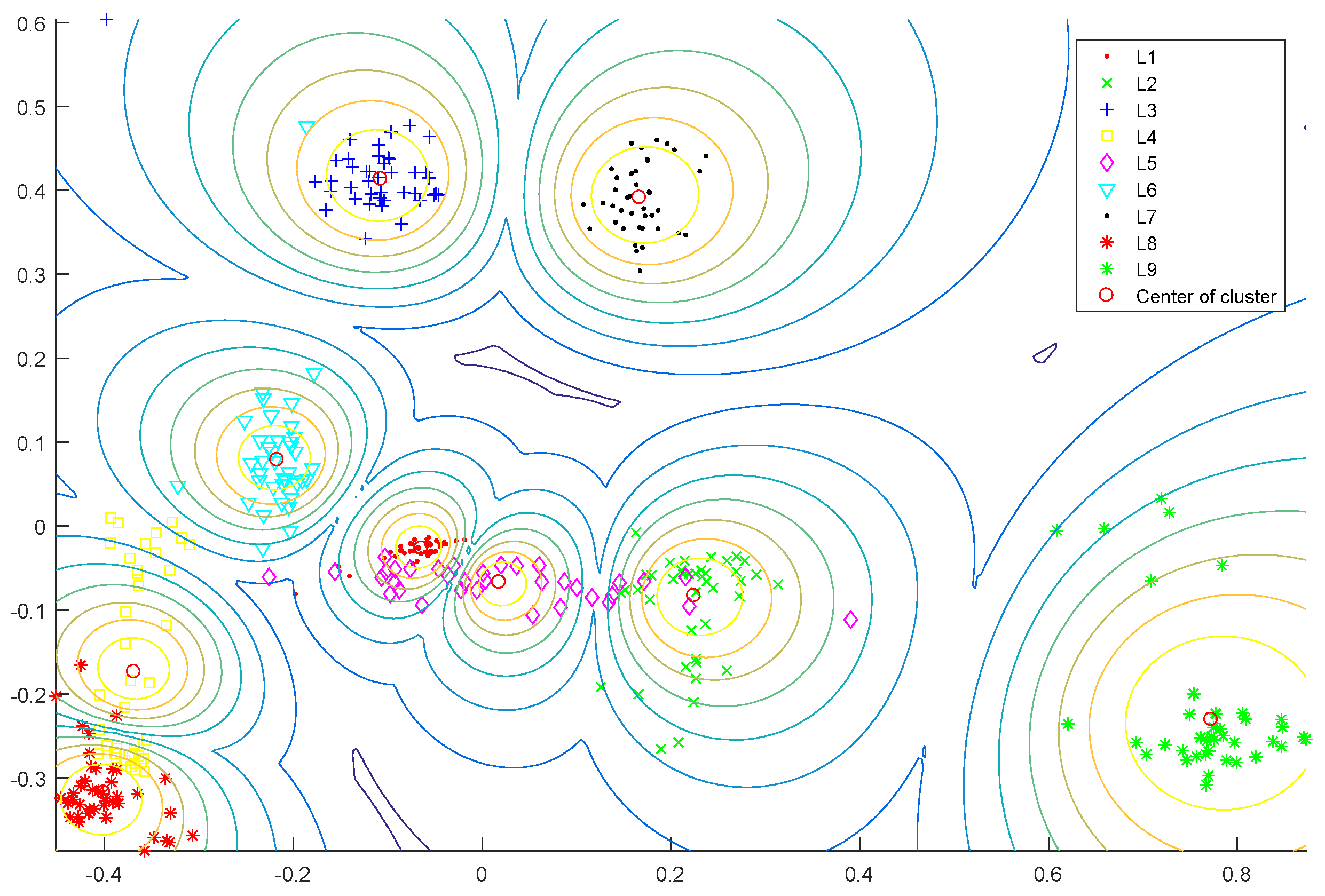
2.3. Semi-Supervised Fuzzy C-Means Clustering

Semi-supervised fuzzy C-means clustering (SSFCM) [18] is an semi-supervised clustering algorithm based on the fuzzy C-means clustering (FCM) algorithm [42]. Specifically, supposing that the sample to be clustered is S = [s₁, s₂, …, s_n] and the number of clusters is c (2 ≤ c ≤ n), then the objective function of SSFCM is given as:

$$J_{w,\alpha }(U,V;S,F)={\displaystyle \sum _{i=1}^c{\displaystyle \sum _{j=1}^n{u}_{ij}^w}{d}_{ij}^2+\rho {\displaystyle \sum _{i=1}^c{\displaystyle \sum _{j=1}^n{(u_{ij}-f_{ij}{b}_j)}^w}}}{d}_{ij}^2$$

(13)

where U_cxn = [u_ij], u_ij represents the fuzzy membership of the jth sample belonging to the ith cluster, and the matrix formed by cluster centers is V = [v₁, v₂, …, v_n]^T. F_cxn = [f_ij], f_ij denotes the membership value of labeled samples, and b_j is a two-valued (Boolean) indicator to distinguish labeled and unlabeled samples. Moreover, d_ij = ||s_j-v_i|| is the Euclidean distance between the jth sample and the ith cluster center, while w (w ≥ 1) is weighting parameter, and 𝜌 (𝜌 ≥ 0) is the balance coefficient.

With Lagrange multipliers introduced, the optimization problem of SSFCM can be converted into the following constrained minimization problem:

$$J_{w,\alpha }(U,V,\lambda ;S,F)={\displaystyle \sum _{i=1}^c{\displaystyle \sum _{j=1}^n{u}_{ij}^w}{d}_{ij}^2+\rho {\displaystyle \sum _{j=1}^n{\displaystyle \sum _{i=1}^c{(u_{ij}-f_{ij}{b}_j)}^w}}}{d}_{ij}^2-{\displaystyle \sum _{j=1}^n{\lambda }_j[{\displaystyle \sum _{i=1}^c(u_{ij}-1)}]}$$

(14)

where λ_j, j = 1, 2, …, n, is the Lagrange multiplier. In the sequel, fuzzy membership u_ij and cluster center v_i can be iterated as:

$$u_{ij}=\frac{1}{1+\rho }[\frac{1+\rho (1-b_j{\displaystyle \sum _{k=1}^c{f}_{kj}})}{{\displaystyle \sum _{k=1}^c{d}_{ij}^2/d_{kj}^2}}+\rho f_{ij}{b}_j]$$

(15)

$$v_i={\displaystyle \sum _{j=1}^n{u}_{ij}^2{s}_j}/{\displaystyle \sum _{j=1}^n{d}_{ij}^2}$$

(16)

where i = 1, 2, …, c, j = 1, 2, …, n.

On the whole, primary procedures of SSFCM can be summarized as follows:

Step 1: Initialize membership matrix U and give values of c, b, F;

Step 2: Calculate prototypical cluster center V;

Step 3: Update U based on Equation (15);

Step 4: Compare U′ to U, if ||U-U′|| < δ (U′ is the last iteration result and δ is a certain tolerance) then loop end, else go to step 2.

2.4. Support Vector Data Description

Support vector data description (SVDD) [25] maps data set into a high-dimensional feature space and deduces a minimum hypersphere which contains as many target objects as possible. Given a target object set x_i, i = 1, 2, …, n, a hypersphere of SVDD can be established. Accordingly, the sphere of the hypersphere can be described by center a and radius R of the sphere. The expression for the hypersphere is as follows:

$$\begin{array}{l}\min f=R^2+C{\displaystyle \sum _i{\xi }_i}\\ s.t.\hspace{0.17em}\hspace{0.17em}\hspace{0.17em}\left|\right|x_i-a|{|}^2\le R^2+{\xi }_i,{\xi }_i\ge 0,\forall i\end{array}$$

(17)

where ξ_i is the slack variable, C is the penalty factor to reach a compromise between the size of hypersphere and number of misclassified samples. By introducing Lagrange multipliers, Equation (17) can be transformed into the following form:

$$L=R^2+C{\displaystyle \sum _i{\xi }_i}-{\displaystyle \sum _i{\alpha }_i(R^2+{\xi }_i-||x_i-a|{|}^2)}-{\displaystyle \sum _i{\beta }_i{\xi }_i}$$

(18)

where α (α ≥ 0) and β (β ≥ 0) are Lagrange multipliers. Finally, a Gaussian radial basis function is applied to replace the inner product, transforming the optimization problem into the following dual problem:

$$\begin{array}{l}\max L={\displaystyle \sum _i{\alpha }_{i}K(x_i,x_i)}-{\displaystyle \sum _{i,j}{\alpha }_i{\alpha }_{j}K(x_i,x_j)}\\ K(x_i,x_j)=\exp (-\frac{\left|\right|x_i-x_j|{|}^2}{{\sigma }^2})\\ s.t.\hspace{0.17em}\hspace{0.17em}{\displaystyle \sum _i{\alpha }_i}=1,\hspace{0.17em}\hspace{0.17em}\hspace{0.17em}\hspace{0.17em}a={\displaystyle \sum _i{\alpha }_i{x}_i,}0\le {\alpha }_i\le C,\hspace{0.17em}\hspace{0.17em}\hspace{0.17em}\hspace{0.17em}\forall i\end{array}$$

(19)

where σ is the kernel parameter.

Solving programming problem (19), α_i is obtained. To be specific, if 0 < α_i < C, the target sample is on the hypersphere, which is called the support vector (SV); if a_i = 0, the sample is in the hypersphere; if α_i = C, the sample is outside the hypersphere, which is called bounded support vector (BSV). For a certain SV x_p, radius of the hypersphere can be calculated as R. For any sample y to be tested, its distance from the center of the hypersphere is D:

$$R^2=K(x_p,x_p)-2{\displaystyle \sum _{i=1}^n{\alpha }_{i}K(x_i,x_p)}+\hspace{0.17em}{\displaystyle \sum _{i,j=1}^n{\alpha }_i\cdot {\alpha }_{j}K(x_i\cdot x_j)}$$

(20)

$$D^2=K(y,y)-2{\displaystyle \sum _{i=1}^n{\alpha }_{i}K(x_i,y)}+{\displaystyle \sum _{i,j=1}^n{\alpha }_i\cdot {\alpha }_{j}K(x_i\cdot x_j)}$$

(21)

3. Fault Diagnosis Based on Semi-Supervised Clustering and Support Vector Data Description with Adaptive Parameter Optimization and Improved Decision Strategy

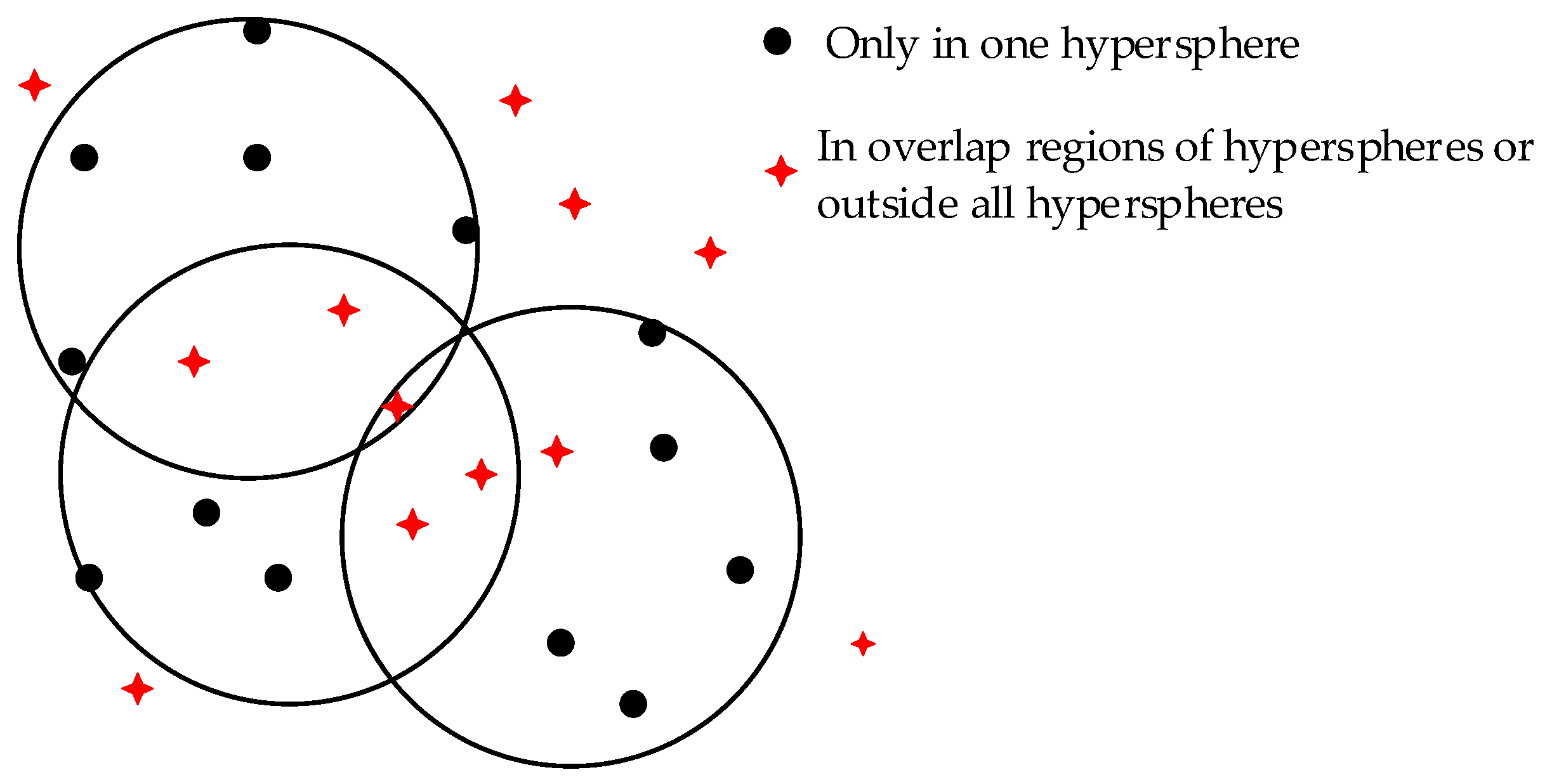
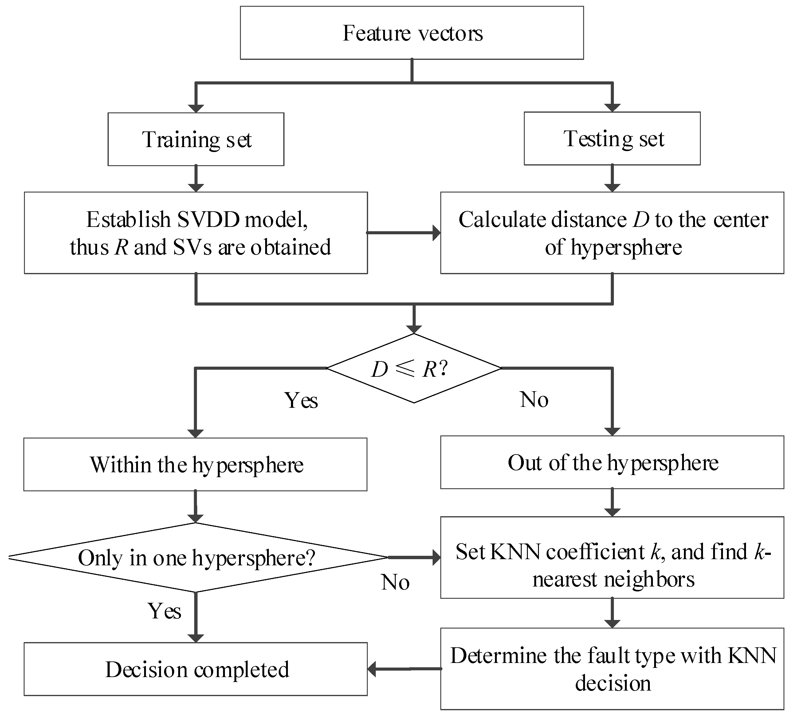
3.1. Improved Decision Strategy

SVDD with relative distance decision strategy (RD-SVDD) is commonly applied for pattern recognition. However, it is difficult for relative distance decision strategy to achieve precise identification, especially for unknown samples within overlap regions of the hyperspheres and regions outside all the hyperspheres. The schematic diagram of positional relationship between samples and hyperspheres is shown in Figure 1. Therefore, further development of decision strategy is required. To this end, SVDD with improved decision strategy (ID-SVDD) that fuses with the k-nearest neighbor (KNN) method is proposed in this research.

The KNN method proposed by Cover et al. [43] is one of the most widely used algorithms for pattern recognition, which is easy to understand and realize. The basic idea of KNN is to measure the differences between samples and their neighbors, and Euclidean and Manhattan distances are usually employed to achieve the measurement. Let p, q be two samples with m terms, the distances between them can be defined as:

$$\begin{array}{cc}\hfill \mathrm{Euclidean}\mathrm{distance}:& D(p,q)=\sqrt{{\displaystyle \sum _{i=1}^m{(p_i-q_i)}^2}}\hfill \end{array}$$

(22)

$$\begin{array}{cc}\hfill \mathrm{Manhattan}\mathrm{distance}:& D(p,q)=\sqrt{{\displaystyle \sum _{i=1}^m\left|p_i-q_i\right|}}\hfill \end{array}$$

(23)

where p_i and q_i are the ith component of p and q respectively.

With training samples labeled by semi-supervised clustering, SVDD models of different types of faults are established, from which hypersphere radiuses Rs and support vectors SVs can also be obtained. Furthermore, by comparing distance D from testing sample to the centers of hyperspheres, it can be judged whether the sample is within the hypersphere. There are two cases after the comparison: If the sample to be classified is only in one hypersphere, the fault type of the sample is directly ascertained; otherwise, if the sample is in the overlap regions of the hyperspheres or regions outside all the hyperspheres, KNN is needed for further classification. To be specific, KNN firstly calculates the distances between testing sample and SVs, finding k-nearest neighbors among SVs whose distances are closest to the testing sample, then the type of the testing sample can be determined according to majority fault types of k-nearest neighbors.

The main steps of ID-SVDD are shown below:

Step 1: Establish SVDD models for different types of faults based on Equations (19) and (20), thus Rs and SVs are obtained;

Step 2: Calculate distance D on the basis of Equation (21);

Step 3: Compare distance D to the radius R of each hypersphere, if testing sample is only in one hypersphere then go to step 6, else go to next step;

Step 4: Set KNN coefficient k, and find k-nearest neighbors according to Equation (22) or (23);

Step 5: Determine the type of testing sample with KNN decision;

Step 6: Decision completed.

The flowchart of ID-SVDD is shown in Figure 2.

3.2. Adaptive Parameter Optimization

3.2.1. Sine Cosine Algorithm

Exploration and exploitation [35] are two phases in which the sine cosine algorithm (SCA) processes the optimization problem. In the phase of exploration, a set of random solutions are initiated as the outset of optimization process. With a strong randomness, SCA is able to search for feasible solutions quickly in the searching space. In the phase of exploitation, the random solutions change gradually, and the randomness is distinctly weaker than that of exploration phase, which is conducive to a better local searching.

Let $Z_i={(Z_{i1},Z_{i2},\dots ,Z_{il})}^T$ be the position of ith (i = 1, 2,…, M) individual, whereupon each solution of the optimization problem corresponds to the position of corresponding individual in the searching space, where l is the dimension of individuals. The best position of individual i is $P_i={(P_{i1},P_{i2},\dots ,P_{il})}^T$. During iterations, the position of individual i will be updated by the following Equations [35]:

$$\begin{array}{l}{Z}_i{}^{k+1}=Z_i{}^k+r_1\times \sin (r_2)\times |r_3{P}_i{}^k-Z_i{}^k|\\ Z_i{}^{k+1}=Z_i{}^k+r_1\times \cos (r_2)\times |r_3{P}_i{}^k-Z_i{}^k|\end{array}$$

(24)

where $Z_i{}^k$ is the position of individual i in kth iteration, r₁, r₂, and r₃ are all random values.

The above equations are synthesized to:

$$Z_i{}^{k+1}=\{\begin{array}{l}{Z}_i{}^k+r_1\times \sin (r_2)\times |r_3{P}_i{}^k-Z_i{}^k|,r_4<0.5\\ Z_i{}^k+r_1\times \cos (r_2)\times |r_3{P}_i{}^k-Z_i{}^k|,r_4\ge 0.5\end{array}$$

(25)

where r₄ is a random value within [0, 1].

As the above equations show, the updating equation has four main parameters, i.e., r₁, r₂, r₃ and r₄. The parameter r₁ contributes to determine the position’s region of individual i at next iteration. The parameter r₂ is a random number in the scope of [0, 2π], which defines distance that next movement should be towards. To stochastically emphasize (r₃ > 1) or deemphasize (r₃ < 1) the effect of the best position of individual, a random weight r₃ within [0, 2] is brought in the equations. Finally, the parameter r₄ is a random number in the range of [0, 1] to switch fairly between sine and cosine components, specifically when r₄ < 0.5, sine component dominates iterations of the position of individual i, otherwise cosine component dominates iterations.

To seek feasible solutions in the searching space and eventually find the global optimum, exploration and exploitation phases should be in a balanced state. For this reason, the amplitudes of the sine and cosine functions are adaptively adjusted by changing $r_1$ as follows [35]:

$$r_1=a-t\frac{a}{T}$$

(26)

where T, t and a are the maximum number of iterations, the current number of iterations and a constant respectively.

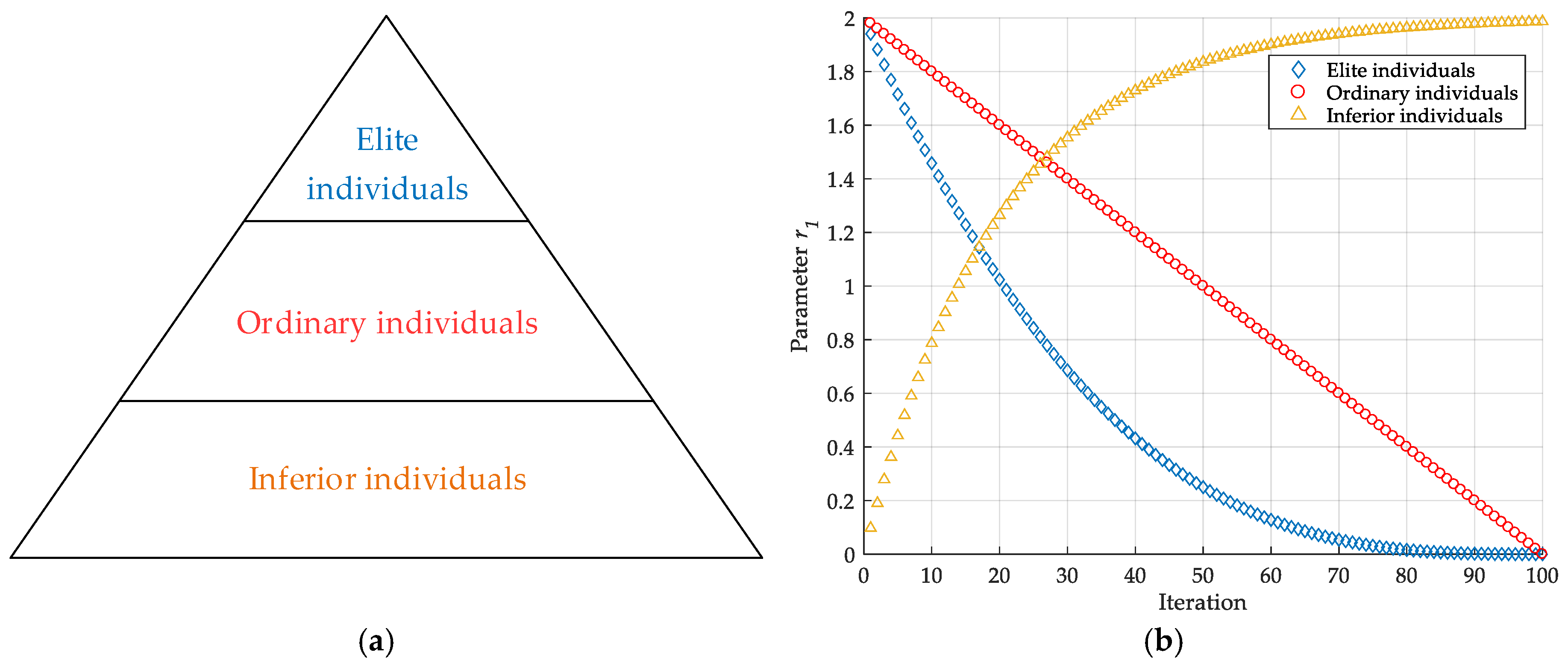
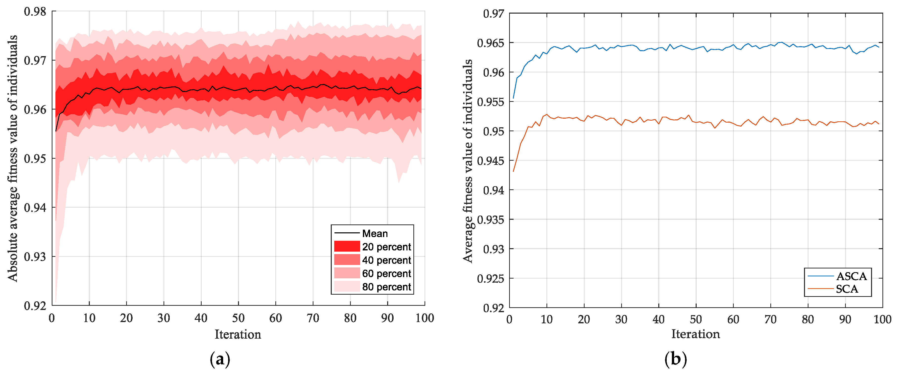
3.2.2. Adaptive Sine Cosine Algorithm

As mentioned in SCA, r₁ is a crucial parameter connecting with the sine and cosine functions r₁sin(r₂) or r₁cos(r₂). On the basis of the design principle of SCA, the algorithm firstly explores different regions and then exploits promising regions. Accordingly, the value of r₁ should be monotone decreasing during iterations. However, the updating strategy of r₁ as shown in Equation (26) is a linear decrease with equal-step, which will restrict the convergence and accuracy. For this purpose, an improved strategy for updating r₁ which is called adaptive sine cosine algorithm (ASCA) is proposed in this paper.

Considering that the fitness values of all individuals would change among the iterations, a hierarchical strategy based on the fitness values of individuals is introduced to divide all individuals into three subgroups [44]. More specifically, let f_i be the fitness value of individual i, f_a be the average fitness value of all individuals, and f_e represents the average fitness value of individuals that fitness value better than f_a. If f_i is better than f_e, individual i is defined as elite individual; if f_i is better than f_a but worse than f_e, individual i is defined as ordinary individual; if f_i is worse than f_a, then define individual i as inferior individual. The hierarchical strategy is illustrated in Figure 3a. After the above process, the number of individuals in different subgroups can be adaptively adjusted according to the fitness values during iterations, and different subgroups implement different adaptive operations. The updating strategy for r₁ is defined as follows and changes of r₁ for individuals of different subgroups is shown in Figure 3b:

(1) Elite individuals: Are the best individuals among all ones, and close to the optimal value. A smaller r₁ is given with a cubic function to enhance local searching:

$$r_1=(r_{\max }-r_{\min }){(\frac{T-t}{T})}^3+r_{\min }$$

(27)

where r_max and r_min are the maximum and minimum value of r₁ respectively, while T and t are the maximum and current number of iterations respectively.

(2) Ordinary individuals: Possess good global and local searching ability. r₁ maintains the original linear decreasing trend:

$$r_1=a-t\frac{a}{T}$$

(28)

(3) Inferior individuals: Are far from the optimal value. A bigger r₁ is needed to enhance global searching in early iteration, and to jump out the local optimum later:

$$r_1=(r_{\min }-r_{\max })e^{-b\frac{t}{T}}+r_{\max }$$

(29)

where b is a positive constant to adjust exponential curve.

3.3. Fault Diagnosis Based on SSFCM and ID-SVDD Optimized by ASCA

In this section, a novel model based on semi-supervised fuzzy C-means clustering, adaptive sine cosine algorithm and support vector data description with improved decision strategy (SSFCM-ASCA-ID-SVDD) is proposed to diagnose faults for rolling bearing. The specific steps are detailed as follows:

Step 1: Collect vibration signals;

Step 2: Determine the mode number K by central frequency observation method;

Step 3: Decompose the signals into sets of IMFs with VMD;

Step 4: Calculate FuzzyEn values of all IMFs, and construct the fault feature vectors of training and testing samples;

Step 5: Cluster training samples by SSFCM, thus the training samples are all labeled;

Step 6: Optimize the parameters C and σ for SVDD with the proposed ASCA;

Step 7: Train the ID-SVDD model with the optimal parameters C and σ;

Step 8: Apply the optimal ID-SVDD model to classify different types of faults and evaluate the performance of the model.

The flowchart of the proposed fault diagnosis model is shown in Figure 4.

4. Engineering Application

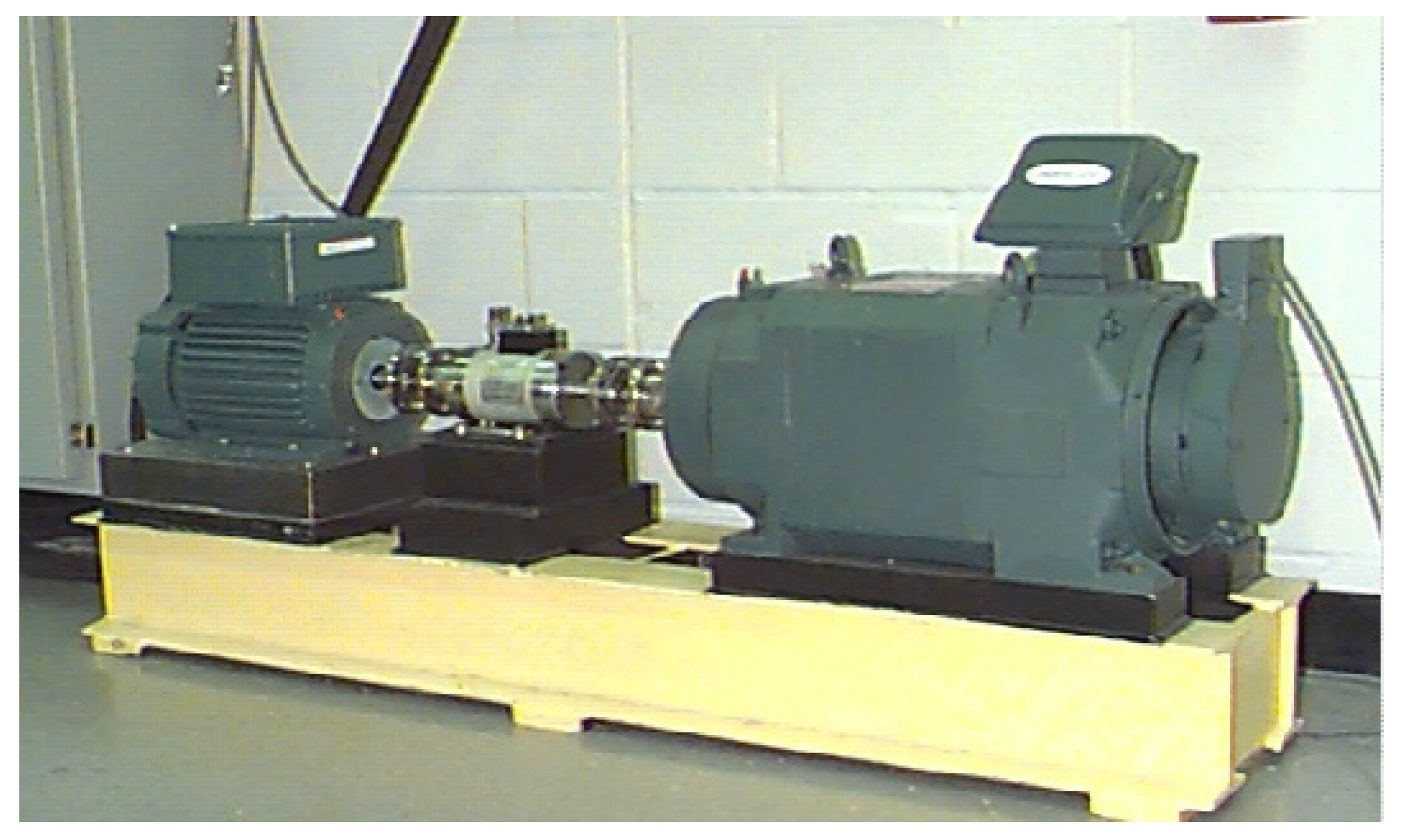
4.1. Data Collection

To validate the performance of the proposed method, a series of vibration signals with different fault locations and sizes were gathered from Bearings Data Center of Case Western Reserve University [45]. The experiment stand was mainly composed of a motor, an accelerometer, a torque sensor/encoder, and a dynamometer. The bearing was a deep groove ball bearing with model SKF6205-2RS. By using electro-discharge machining (EDM), the experiment device simulated three fault states of the rolling bearing: The inner race fault, ball element fault, and outer race fault. The depth of faults was 0.011 inches. Vibration signals collected from the drive end (DE) were taken as the research objects. In the experiment, the sample frequency was 12,000 Hz, and the rotation speed was 1750 rpm under the rated load of 2 hp. To fully verify the validity of the proposed fault diagnosis method, 9 types of samples were used in this paper, namely, the inner race fault, ball fault, and outer race fault with diameters of 0.007, 0.014, and 0.021 inches (i.e., each of the three types of faults has three defect sizes). Further, the vibration signal of each type of fault was divided into 59 segments containing 2048 sampling points. An image of the experiment device is shown in Figure 5. The experimental signals are listed in

Table 1. List of the vibration samples used in the experiment.

Fault Location	Diameter (inches)	Fault Label	Number of Samples
Inner race	0.007	L1	59
Inner race	0.014	L2	59
Inner race	0.021	L3	59
Ball	0.007	L4	59
Ball	0.014	L5	59
Ball	0.021	L6	59
Outer race	0.007	L7	59
Outer race	0.014	L8	59
Outer race	0.021	L9	59

.

4.2. Application to Fault Diagnosis of Rolling Bearing

In order to demonstrate the effectiveness of the proposed SSFCM-ASCA-ID-SVDD method, experiments were implemented by contrast with constrained-K-means (CK-means) [46] in the clustering phase and with SCA in the parameter optimization phase. Similarly, support vector machine (SVM) and SVDD with relative distance decision strategy (RD-SVDD) were applied for comparison during decision making phase. In the proposed method, the first step was to decompose the signal of each type of fault into a set of components with VMD, whose mode number K needed to be determined in advance with central frequency observation method. If the value of K is too large, center frequencies of adjacent IMFs may be too close, and mode mixing will emerge. The center frequencies of all IMFs when taking different K are listed in

Table 2. Center frequencies with different K value.

Number of Modes	Center Frequencies (Hz)
2	2903.44	1166.73
3	3832.19	2928.05	1285.99
4	3179.09	2236.65	1107.20	163.33
5	3945.87	3647.07	2922.65	1477.51	675.67
6	3952.42	3672.88	3042.01	2756.44	1465.45	668.06
7	4079.22	3835.39	3547.95	2921.58	1597.69	1263.47	633.97
8	4088.98	3848.10	3573.75	3040.86	2762.20	1583.65	1255.25	632.93
9	5175.26	4031.42	3821.29	3562.16	3040.24	2761.83	1583.05	1254.80	633.18

, where K was ascertained by the sample of inner race fault with diameter of 0.007 inches (L1). As illustrated in Table 2, when K was set to 5, the first two center frequencies were relatively close, which meant that excessive decomposition occurred. The same conclusion can also be seen in Figure 6, during the iterative calculation of VMD, if K was 5 or greater, some center frequencies of IMFs would be relatively close to each other. For example, when K was 5, IMF₁ and IMF₂ were relatively close, while K was 6, IMF₂ and IMF₃ were relatively close. Therefore, parameter K was set to 4 in this research.

The decomposition results of samples with different fault types are illustrated in Figure 7, from which it can be seen that waveforms of different fault samples are different to some extent. After VMD decomposition, FuzzyEn values were calculated to construct the fault feature vectors, and the fractal dimension m was set 2 while the positive real number r was set as 0.2. The first three FuzzyEn vectors of different fault samples (L1–L9) are reported in

Table 3. Fuzzy entropy values of different fault samples.

Fault Label	Sample Number	Fuzzy Entropy for Different IMFs
		IMF1	IMF2	IMF3	IMF4
L1	1	1.7996	1.8052	1.1744	0.6738
	2	1.7691	1.8104	1.1649	0.6638
	3	1.8286	1.7767	1.1695	0.6738
L2	1	1.7242	1.3599	1.1695	0.5838
	2	1.6353	1.2388	1.1776	0.5799
	3	1.6377	1.3705	1.1981	0.6119
L3	1	2.0356	1.6703	1.8310	0.6125
	2	1.9168	1.7186	1.8202	0.6199
	3	1.9248	1.7081	1.8325	0.6094
L4	1	2.2160	2.0236	0.9334	0.3960
	2	2.2282	2.0723	0.9072	0.3288
	3	2.2025	2.0116	0.9650	0.5454
L5	1	1.7123	1.6451	1.2169	0.4758
	2	1.9905	1.6487	1.1966	0.4806
	3	1.9124	1.6921	1.1990	0.4936
L6	1	1.7338	2.0930	1.2618	0.6195
	2	2.1333	1.9824	1.2164	0.6141
	3	2.1229	1.9946	1.2435	0.6438
L7	1	1.2859	1.7536	1.5843	0.9124
	2	1.2313	1.7508	1.6109	0.8821
	3	1.3335	1.7556	1.6099	1.0993
L8	1	2.1004	2.0725	0.8502	0.4750
	2	2.1927	2.1651	0.7906	0.4937
	3	2.1565	2.1261	0.9207	0.5691
L9	1	0.7437	0.9596	0.9206	0.4920
	2	0.6916	1.0609	1.2533	0.5486
	3	0.9297	0.9185	0.9081	0.5329

.

The feature vectors of samples from different fault types were divided randomly into two parts with 40 and 19 vectors, respectively, the first part was used for training and the second one for testing. In order to better illustrate the characteristics and effects of SSFCM, training samples with ratio of 0.3 and 0.5 were randomly selected as labeled samples, while the rest were samples with unknown fault types. The weighting parameter w of SSFCM was set to 2 while the balance coefficient α was set to 1/0.3 and 1/0.5, respectively, according to the ratio. Figure 8 depicts the 2D projection of training samples after clustering. The figure shows that training samples are gathered into nine clusters under the supervision of labeled samples and distributed near the center of each cluster. The contour-map displays the samples with the same partitioning values.

In the optimization phase, the proposed ASCA approach was applied to optimize the penalty factor C and the kernel parameter σ, where the individual number was set to 30 and iteration times were set to 100. Considering the constraints of the optimization problem of SVDD, C should subject to C ≥ 1/n, where n is the number of target objects. Likewise, C should be subject to C < 1 or else it loses constraint on Lagrange multipliers. Taken together, searching ranges of C and σ were [1/n, 1] and [2⁻¹⁰, 2¹⁰], respectively. The coefficient k was set to 3 for KNN decision. During optimization process, the fitness value was calculated by five-fold cross validation on the training samples.

The optimization effect with the given (C, σ) was measured by average accuracy of cross validation, then the optimal (C, σ) was obtained. The convergence procedure of the adaptive parameter optimization is depicted in Figure 9a. It can be seen that the absolute average fitness value of all individuals increases rapidly at early stage of iterations and then tends to be stable, which means the individuals were moving closer to the global optimal solution. The shaded part shows the distribution of the convergence curve in 10 optimization experiments. The comparison of ASCA and SCA is shown in Figure 9b, where all convergence experiments use the same FuzzyEn values and each convergence curve is the average of 10 experiments. The figure shows that both ASCA and SCA have a good convergence effect, but ASCA keeps a better convergence effect than SCA in the whole iterations. Besides, in the middle and later stages of iterations, the convergence curve of SCA decreases slightly, while ASCA remains stable.

With the optimal parameters (C, σ) and labeled training samples, the ID-SVDD model was trained and applied to recognize testing samples. For an in-depth verification of the proposed method, diagnosis results were averaged over 10 runs and the training samples were chosen at random in every run. In this application, normalized mutual information (NMI) as well as accuracy (ACC) as two widely used evaluation metrics are employed to evaluate the diagnosis results [47], which reflects the matching degree between classification results and real sample distribution information. The scope of two metrics is both [0, 1]. The value closer to 1 indicates a better classification performance of the model. In addition, corresponding deviation scope for each result was also calculated as a reference for evaluation. The optimal (C, σ) is presented corresponding to the best accuracy among 10 runs.

In contrastive experiments, parameters of CK-means, SCA, and RD-SVDD were set similar to the proposed method. That is, training samples with a ratio of 0.3 and 0.5 were randomly selected as labeled samples for CK-means clustering; SCA had 30 individuals and iterated 100 times; the ranges of C and σ of RD-SVDD were [1/n, 1] and [2⁻¹⁰, 2¹⁰] respectively. Considering the difference between SVDD and SVM, the searching scopes of parameter C and g of SVM were both set as [2⁻¹⁰, 2¹⁰] respectively. Moreover, the optimal parameters C and σ(g) of all contrastive methods were selected in the same way the proposed method done. The performance of all contrastive methods was evaluated by NMI and ACC as well. A list of all important parameters in the experiment is shown in

Table 4. Value of parameter in the experiment.

Parameter	Description	Method	Value
K	mode number	VMD	4
m	fractal dimension	FuzzyEn	2
r	positive real number	FuzzyEn	0.2
w	weighting parameter	SSFCM	2
α	balance coefficient	SSFCM	1/0.3 and 1/0.5
M	number of individuals	ASCA	30
T	iteration times	ASCA	100
C	penalty factor	SVDD	0.1177 and 0.1523
σ	kernel parameter	SVDD	26.7073 and 0.0011
k	number of nearest neighbors	KNN	3

.

The fault diagnosis results with different methods are shown in

Table 5. Fault diagnosis results with different methods.

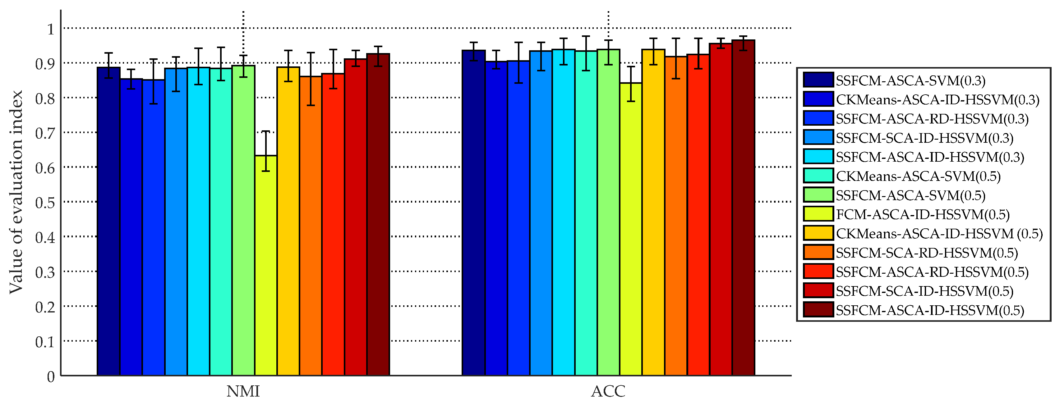
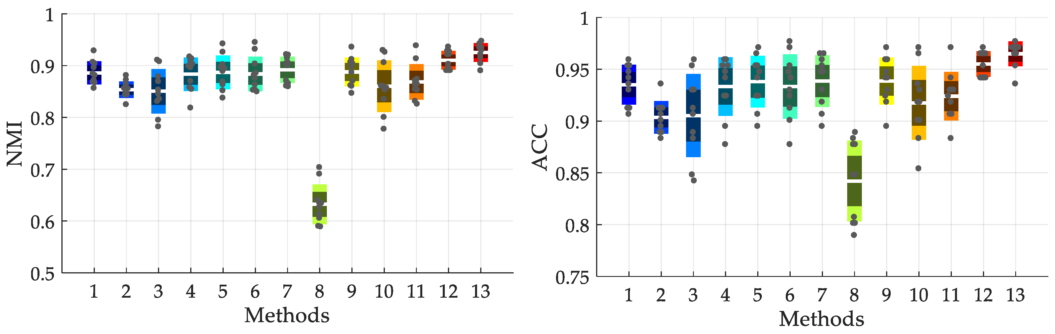
Processing Methods (Labeled Ratio)	C	σ (g)	Result Evaluation
			Normalized Mutual Information (NMI)	Accuracy (ACC)
SSFCM-ASCA-SVM (0.3)	39.8545	3.4262	0.8860, [−0.030, 0.042]	0.9351, [−0.029, 0.024]
CK-means-ASCA-ID-SVDD (0.3)	0.0983	72.2803	0.8534, [−0.029, 0.027]	0.9035, [−0.020, 0.032]
SSFCM-ASCA-RD-SVDD (0.3)	0.0323	1024.0000	0.8505, [−0.069,0.060]	0.9053, [−0.063, 0.054]
SSFCM-SCA-ID-SVDD (0.3)	0.9560	29.5815	0.8833, [−0.065, 0.033]	0.9333, [−0.056, 0.026]
SSFCM-ASCA-ID-SVDD (0.3)	0.1177	26.7073	0.8868, [−0.050, 0.055]	0.9380, [−0.043, 0.033]
CK-means-ASCA-SVM (0.5)	31.4351	1.2567	0.8838, [−0.035, 0.061]	0.9333, [−0.056, 0.043]
SSFCM-ASCA-SVM (0.5)	73.4361	0.2825	0.8919, [−0.044, 0.071]	0.9386, [−0.044, 0.026]
FCM-ASCA-ID-SVDD (0.5)	0.9892	1005.0437	0.6323, [−0.044, 0.071]	0.8421, [−0.053, 0.047]
CK-means-ASCA-ID-SVDD (0.5)	0.0303	0.0025	0.8877, [−0.041, 0.048]	0.9386, [−0.044, 0.032]
SSFCM-SCA-RD-SVDD (0.5)	0.5104	0.1006	0.8601, [−0.083, 0.069]	0.9175, [−0.064, 0.053]
SSFCM-ASCA-RD-SVDD (0.5)	0.2456	18.3967	0.8686, [−0.043, 0.070]	0.9240, [−0.041, 0.047]
SSFCM-SCA-ID-SVDD (0.5)	0.8195	51.0377	0.9102, [−0.020, 0.026]	0.9550, [−0.013, 0.016]
SSFCM-ASCA-ID-SVDD (0.5)	0.1523	0.0011	0.9254, [−0.036, 0.021]	0.9649, [−0.029, 0.012]

and Figure 10. It can be seen from Table 5 that the proposed SSFCM-ASCA-ID-SVDD method achieves the best performance in terms of NMI and ACC metrics among all methods, i.e., 0.0868 and 0.9333 when the ratio is 0.3, 0.9254 and 0.09649 when the ratio is 0.5. To be specific, in the case of the ratio of 0.5: The comparison of FCM-ASCA-ID-SVDD, CK-means-ASCA-ID-SVDD and the proposed method indicates that NMI value of proposed method is 0.2913 and 0.0377 higher than other two methods, as well as that ACC value is 0.1228 and 0.0263 higher than other two methods, which shows SSFCM possess a better clustering precision. Similarly, the comparison analysis between SSFCM-SCA-ID-SVDD and the proposed method shows that ASCA-optimized ID-SVDD improves NMI value by 0.0152 and ACC value by 0.0099 than SCA-optimized ID-SVDD, indicating the effectiveness of the proposed adaptive parameter optimization strategy. Furthermore, the contrast among SSFCM-ASCA-SVM, SSFCM-ASCA-RD-SVDD and the proposed method shows that the NMI evaluation of proposed method is 0.0335 and 0.0568 higher than that of other two methods, while the ACC evaluation of proposed method is 0.0263 and 0.0409 higher than that of other two methods. Thus, it can be concluded that the proposed ID-SVDD model with improved decision strategy has better diagnosis performance.

Additionally, through the comprehensive analysis with a labeled sample ratio of 0.3 and 0.5, it showed that the proposed method achieved the best results under both the two ratio conditions. Meanwhile, the metrics under a ratio of 0.5 was better than that under a ratio of 0.3, which manifests that the clustering performance of SSFCM would be improved with the increasing of the labeled ratio, thus improving the diagnostic accuracy. Figure 11 is the boxplots of evaluation values, illustrating the performance of different diagnosis methods. As shown in the figure, the proposed SSFCM-ASCA-ID-SVDD method achieves a higher precision and possess better stability than other contrastive methods.

5. Discussion

The superiority of the proposed ASCA and ID-SVDD methods have been effectively demonstrated by the above analysis. Likewise, the accuracy of the diagnosis model has also been verified by contrastive experiments on various fault sizes and locations. This preliminary study mainly deals with the fault diagnosis of vibration signals on the rated load. For the practical application in real industrial operating conditions, variable load conditions should also be considered. Those application situations will be researched in our future work. Besides, the proposed ASCA algorithm can be optimized through better strategies to further improve the convergence speed and global search ability. Moreover, the multi-objective optimization that has been widely utilized in the field of controlling [48,49,50] could be implemented in fault diagnosis, which is expected to improve the accuracy and reduce the variance of the outputs of the model [51].

6. Conclusions

A novel fault diagnosis method for rotating bearing based on semi-supervised clustering and support vector data description with adaptive parameter optimization and improved decision strategy is presented in this study. Due to the non-stationarity of the original signals, signals collected from different types of faults were firstly split by VMD into sets of IMFs, before which process, the decomposing mode number K was determined by central frequency observation method. Next, the FuzzyEn values of all IMFs were calculated to construct the feature vectors of different types of faults. Subsequently, all training samples were labeled by using SSFCM under the supervision of partly labeled samples. Finally, SVDD with adaptive parameter optimization and improved decision strategy, i.e., ASCA-ID-SVDD, was proposed to diagnose different fault samples. In an engineering application, the contrastive experiments were implemented between the proposed SSFCM-ASCA-ID-SVDD method and other relevant methods. In the sequel, nine types of faults with different locations and sizes were successfully diagnosed, and the results show that the proposed method exhibited the best performance in both NMI and ACC evaluations. Particularly, when training samples with the ratio of 0.5 that are randomly selected as the labeled samples, the NMI value of the proposed method is 0.0335, 0.2913, 0.0377, 0.0568, and 0.0152 higher than that of SSFCM-ASCA-SVM, FCM-ASCA-ID-SVDD, CK-means-ASCA-ID-SVDD, SSFCM-ASCA-RD-SVDD, and SSFCM-SCA-ID-SVDD respectively. Likewise, the ACC value of the proposed method is 0.0263, 0.1228, 0.0263, 0.0409, and 0.0099 higher than that of other methods respectively. Moreover, the boxplots of different methods illustrate the precision and stability of the proposed method. In summary, the proposed method shows better superiority to other methods and achieves preferable diagnostic performance.

References

- Yi, C.; Lv, Y.; Xiao, H.; You, G.; Dang, Z. Research on the blind source separation method based on regenerated phase-shifted sinusoid-assisted EMD and its application in diagnosing rolling-bearing faults. Appl. Sci. 2017, 7, 414. [Google Scholar] [CrossRef]
- Riaz, S.; Elahi, H.; Javaid, K.; Shahzad, T. Vibration feature extraction and analysis for fault diagnosis of rotating machinery-a literature survey. Asia Pac. J. Multidiscip. Res. 2017, 5, 103–110. [Google Scholar]
- Mbo’O, C.P.; Hameyer, K. Fault diagnosis of bearing damage by means of the linear discriminant analysis of stator current features from the frequency selection. IEEE Trans. Ind. Appl. 2016, 52, 3861–3868. [Google Scholar] [CrossRef]
- Yuan, R.; Lv, Y.; Song, G. Fault diagnosis of rolling bearing based on a novel adaptive high-order local projection denoising method. Complexity 2018, 2018, 3049318. [Google Scholar] [CrossRef]
- Fu, W.; Tan, J.; Li, C.; Zou, Z.; Li, Q.; Chen, T. A hybrid fault diagnosis approach for rotating machinery with the fusion of entropy-based feature extraction and SVM optimized by a chaos quantum sine cosine algorithm. Entropy 2018, 20, 626. [Google Scholar] [CrossRef]
- Adamczak, S.; Stepien, K.; Wrzochal, M. Comparative study of measurement systems used to evaluate vibrations of rolling bearings. Procedia Eng. 2017, 192, 971–975. [Google Scholar] [CrossRef]
- Kankar, P.K.; Sharma, S.C.; Harsha, S.P. Rolling element bearing fault diagnosis using wavelet transform. Neurocomputing. 2011, 74, 1638–1645. [Google Scholar] [CrossRef]
- Ali, J.B.; Fnaiech, N.; Saidi, L.; Chebel-Morello, B.; Fnaiech, F. Application of empirical mode decomposition and artificial neural network for automatic bearing fault diagnosis based on vibration signals. Appl. Acoust. 2015, 89, 16–27. [Google Scholar]
- Fu, W.; Zhou, J.; Zhang, Y.; Zhu, W.; Xue, X.; Xu, Y. A state tendency measurement for a hydro-turbine generating unit based on aggregated EEMD and SVR. Meas. Sci. Technol. 2015, 26, 125008. [Google Scholar] [CrossRef]
- Li, K.; Su, L.; Wu, J.; Wang, H.; Chen, P. A rolling bearing fault diagnosis method based on variational mode decomposition and an improved kernel extreme learning machine. Appl. Sci. 2017, 7, 1004. [Google Scholar] [CrossRef]
- Fu, W.; Wang, K.; Li, C.; Li, X.; Li, Y.; Zhong, H. Vibration trend measurement for a hydropower generator based on optimal variational mode decomposition and an LSSVM improved with chaotic sine cosine algorithm optimization. Meas. Sci. Technol. 2019, 30, 015012. [Google Scholar] [CrossRef]
- Fu, W.; Wang, K.; Zhou, J.; Xu, Y.; Tan, J.; Chen, T. A hybrid approach for multi-step wind speed forecasting based on multi-scale dominant ingredient chaotic analysis, KELM and synchronous optimization strategy. Sustainability 2019, 11, 1804. [Google Scholar] [CrossRef]
- Xie, H.; Sivakumar, B.; Boonstra, T.W.; Mengersen, K. Fuzzy entropy and its application for enhanced subspace filtering. IEEE Trans. Fuzzy Syst. 2018, 26, 1970–1982. [Google Scholar] [CrossRef]
- Li, Y.; Xu, M.; Wang, R.; Huang, W. A fault diagnosis scheme for rolling bearing based on local mean decomposition and improved multiscale fuzzy entropy. J. Sound Vib. 2016, 360, 277–299. [Google Scholar] [CrossRef]
- Zhu, X.; Zheng, J.; Pan, H.; Bao, J.; Zhang, Y. Time-shift multiscale fuzzy entropy and laplacian support vector machine based rolling bearing fault diagnosis. Entropy 2018, 20, 602. [Google Scholar] [CrossRef]
- Fu, W.; Tan, J.; Zhang, X.; Chen, T.; Wang, K. Blind parameter identification of MAR model and mutation hybrid GWO-SCA optimized SVM for fault diagnosis of rotating machinery. Complexity 2019, 2019, 3264969. [Google Scholar] [CrossRef]
- Cerrada, M.; Sánchez, R.; Li, C.; Pacheco, F.; Cabrera, D.; José, V.D.O.; Vásquez, R.E. A review on data-driven fault severity assessment in rolling bearings. Mech. Syst. Signal Process. 2018, 99, 169–196. [Google Scholar] [CrossRef]
- Pedrycz, W. Algorithms of fuzzy clustering with partial supervision. Pattern Recognit. Lett. 1985, 3, 13–20. [Google Scholar] [CrossRef]
- Xu, C.; Zhang, P.; Ren, G.; Fu, J. Engine wear fault diagnosis based on improved semi-supervised fuzzy C-means clustering. J. Mech. Eng. 2011, 47, 55. [Google Scholar] [CrossRef]
- Arshad, A.; Riaz, S.; Jiao, L. Semi-supervised deep fuzzy c-mean clustering for imbalanced mulit-class classification. IEEE Access 2019, 7, 28100–28112. [Google Scholar] [CrossRef]
- Yao, B.; Su, J.; Wu, L.; Guan, Y. Modified local linear embedding algorithm for rolling element bearing fault diagnosis. Appl. Sci. 2017, 7, 1178. [Google Scholar] [CrossRef]
- Raj, N.; Jagadanand, G.; George, S. Fault detection and diagnosis in asymmetric multilevel inverter using artificial neural network. Int. J. Electron. 2017, 105, 559–571. [Google Scholar] [CrossRef]
- Chen, H.; Wang, J.; Li, J.; Tang, B. A texture-based rolling bearing fault diagnosis scheme using adaptive optimal kernel time frequency representation and uniform local binary patterns. Meas. Sci. Technol. 2017, 28, 035903. [Google Scholar] [CrossRef]
- Wang, H.; Chen, J. Performance degradation assessment of rolling bearing based on bispectrum and support vector data description. J. Vib. Control 2014, 20, 2032–2041. [Google Scholar] [CrossRef]
- Tax, D.M.J.; Duin, R.P.W. Support vector data description. Mach. Learn. 2004, 54, 45–66. [Google Scholar] [CrossRef]
- Zhou, J.; Fu, W.; Zhang, Y.; Xiao, H.; Xiao, J.; Zhang, C. Fault diagnosis based on a novel weighted support vector data description with fuzzy adaptive threshold decision. Trans. Inst. Measure. Control 2018, 40, 71–79. [Google Scholar] [CrossRef]
- Zhou, J.; Guo, H.; Zhang, L.; Xu, Q.; Li, H. Bearing performance degradation assessment using lifting wavelet packet symbolic entropy and SVDD. Shock Vib. 2016, 2016, 1–10. [Google Scholar] [CrossRef]
- Wang, H. Fault diagnosis of rolling element bearing compound faults based on sparse no-negative matrix factorization-support vector data description. J. Vib. Control 2018, 24, 272–282. [Google Scholar] [CrossRef]
- Liu, Y.; Qin, H.; Zhang, Z.; Yao, L.; Wang, C.; Mo, L.; Ouyang, S.; Li, J. A region search evolutionary algorithm for many-objective optimization. Inform. Sci. 2019. [Google Scholar] [CrossRef]
- Fu, W.; Tan, J.; Xu, Y.; Wang, K.; Chen, T. Fault diagnosis for rolling bearings based on fine-sorted dispersion entropy and SVM optimized with mutation SCA-PSO. Entropy 2019, 21, 404. [Google Scholar] [CrossRef]
- Zhang, C.; Peng, T.; Li, C.; Fu, W.; Xia, X.; Xue, X. Multiobjective optimization of a fractional-order PID controller for pumped turbine governing system using an improved NSGA-III algorithm under multiworking conditions. Complexity 2019, 2019, 5826873. [Google Scholar] [CrossRef]
- Duan, L.; Xie, M.; Bai, T.; Wang, J. A new support vector data description method for machinery fault diagnosis with unbalanced datasets. Expert Syst. Appl. 2016, 64, 239–246. [Google Scholar] [CrossRef]
- Xu, Y.; Zheng, Y.; Du, Y.; Yang, W.; Peng, X.; Li, C. Adaptive condition predictive-fuzzy PID optimal control of start-up process for pumped storage unit at low head area. Energy Convers. Manag. 2018, 177, 592–604. [Google Scholar] [CrossRef]
- Xu, Y.; Li, C.; Wang, Z.; Zhang, N.; Peng, B. Load frequency control of a novel renewable energy integrated micro-grid containing pumped hydropower energy storage. IEEE Access 2018, 6, 29067–29077. [Google Scholar] [CrossRef]
- Mirjalili, S. SCA: A sine cosine algorithm for solving optimization problems. Knowl.-Based Syst. 2016, 96, 120–133. [Google Scholar] [CrossRef]
- Fu, W.; Wang, K.; Li, C.; Tan, J. Multi-step short-term wind speed forecasting approach based on multi-scale dominant ingredient chaotic analysis, improved hybrid GWO-SCA optimization and ELM. Energy Convers. Manag. 2019, 187, 356–377. [Google Scholar] [CrossRef]
- Elaziz, M.A.; Oliva, D.; Xiong, S. An improved opposition-based sine cosine algorithm for global optimization. Expert Syst. Appl. 2017, 90, 484–500. [Google Scholar] [CrossRef]
- Dragomiretskiy, K.; Zosso, D. Variational mode decomposition. IEEE Trans. Signal Process. 2014, 62, 531–544. [Google Scholar] [CrossRef]
- Chan, R.H.; Tao, M.; Yuan, X. Constrained total variation deblurring models and fast algorithms based on alternating direction method of multipliers. SIAM J. Imaging Sci. 2013, 6, 680–697. [Google Scholar] [CrossRef]
- Richman, J.S.; Moorman, J.R. Physiological time-series analysis using approximate entropy and sample entropy. Am. J. Physiol. Heart Circ. Phys. 2000, 278, H2039–H2049. [Google Scholar] [CrossRef]
- Chen, W.; Wang, Z.; Xie, H.; Yu, W. Characterization of surface EMG signal based on fuzzy entropy. IEEE Trans. Neural Syst. Rehabil. Eng. 2007, 15, 266–272. [Google Scholar] [CrossRef] [PubMed]
- Bezdek, J.C.; Ehrlich, R.; Full, W. FCM: The fuzzy c -means clustering algorithm. Comput. Geosci. 1984, 10, 191–203. [Google Scholar] [CrossRef]
- Cover, T.; Hart, P. Nearest neighbor pattern classification. IEEE Trans. Inf. Theory 1967, 13, 21–27. [Google Scholar] [CrossRef]
- Wu, H.; Zhu, C.; Chang, B.; Liu, J. Adaptive genetic algorithm to improve group premature convergence. J. Xi’an Jiaotong Univ. 1999, 33, 27–30. (In Chinese) [Google Scholar]
- Bearing Data Center of the Case Western Reserve University. Available online: http://csegroups.case.edu/bearingdatacenter/pages/download-data-file (accessed on 28 September 2018).
- Basu, S.; Banerjee, A.; Mooney, R.J. Semi-supervised clustering by seeding. In Proceedings of the Nineteenth International Conference on Machine Learning, Sydney, Australia, 8–12 July 2002; pp. 19–26. [Google Scholar]
- Fahad, A.; Alshatri, N.; Tari, Z.; Alamri, A.; Khalil, I.; Zomaya, A.Y.; Foufou, S.; Bouras, A. A survey of clustering algorithms for big data: Taxonomy and empirical analysis. IEEE Trans. Emerg. Top. Comput. 2014, 2, 267–279. [Google Scholar] [CrossRef]
- Lai, X.; Li, C.; Zhou, J.; Zhang, N. Multi-objective optimization for guide vane shutting based on MOASA. Renew. Energy 2019, 139, 302–312. [Google Scholar] [CrossRef]
- Li, C.; Wang, W.; Chen, D. Multi-objective complementary scheduling of hydro-thermal-RE power system via a multi-objective hybrid grey wolf optimizer. Energy 2019, 171, 241–255. [Google Scholar] [CrossRef]
- Liu, Y.; Qin, H.; Mo, L.; Wang, Y.; Chen, D.; Pang, S.; Yin, X. Hierarchical flood operation rules optimization using multi-objective cultured evolutionary algorithm based on decomposition. Water Resour. Manag. 2019, 33, 337–354. [Google Scholar] [CrossRef]
- Jiang, L.; Xuan, J.; Shi, T. Feature extraction based on semi-supervised kernel marginal fisher analysis and its application in bearing fault diagnosis. Mech. Syst. Signal Process. 2013, 41, 113–126. [Google Scholar] [CrossRef]