Abstract
Failure mode and effect analysis (FMEA) is one of the most widely employed pre-evaluation techniques to avoid risks that may occur during product design and manufacturing phases. However, use of the risk priority number (RPN) in traditional FMEA results in difficulties being encountered with regard to quantification of the degree of risk involved. This study proposes the use of a probabilistic time-dependent FMEA (TD-FMEA) approach to overcome limitations encountered during implementation of traditional FMEA approaches. To this end, the proposed method defines the risk priority metric (RPM) as a priority decision value. RPM corresponds to the product of the expected loss and occurrence rate of the failure-cause. By assuming exponential and case functions for each occurrence and detection time instant, the expected loss corresponding to each failure-cause can be evaluated. Utility of the proposed approach has been described in the light of results obtained via its implementation during an automotive-manufacturing case study performed for the purpose of illustration.
1. Introduction
Failure mode and effect analysis (FMEA) is an analysis technique for defining, identifying, and eliminating known and/or potential failures, problems, errors, etc. from systems, designs, processes, and/or services before they reach the customer [1]. The results of the FMEA can help analysts to identify and correct the failure modes that have a detrimental effect on the system and improve its performance during the stages of design and production [2]. Since its introduction as an analysis tool for reducing failures, FMEA has been extensively used in a wide range of industries, including automotive, semiconductor, aircraft medical, and steel industries [3,4,5,6].
In traditional FMEA approaches, the risk associated with a failure-cause is usually evaluated using the risk priority number (RPN), which corresponds to the mathematical product of the occurrence (O), severity (S), and detection (D) of a failure-cause (i.e., RPN = O × S × D, where O is related to failure occurrence, D to failure detection, and S to failure severity). RPN evaluation of a potential failure-cause requires evaluation of three risk factors via the use of the 1-to-10 scale. The higher the RPN of a failure-cause, the greater is the associated risk with regard to system/product reliability. However, this traditional FMEA risk-evaluation approach has often been extensively criticized in extant literature for a variety of reasons [2]. Noteworthy drawbacks of the traditional RPN-based approach include (i) no consideration of relative importance among O, S, and D parameters [7,8,9,10]; (ii) difficulties involved in precise evaluation of the three risk factors [5,11,12,13,14,15,16,17]; (iii) no consideration of interdependencies among different failure-causes and the corresponding effects [6,18,19,20]; and (iv) over-dependence on expert intuition and experience instead of scientific methods for evaluation of the three risk components [21,22].
Many researchers have attempted to overcome the above-mentioned drawbacks, thereby improving the FMEA risk-evaluation method in the process. Liu et al. [2] reported that the most popular FMEA approach corresponds to the fuzzy rule-based system [10,23,24,25], followed by the grey theory [9,10], cost-based model [11,12,13], AHP/ANP [7,19,26,27], and linear programming. Others included an integration-based approach [8,15,16,17,21,22,28] and probability-based methodology [14,29]. Apart from these approaches, the use of a time-dependent probabilistic approach for FMEA risk-evaluation has been proposed in this study. In the proposed model, two additional factors—time (failure occurrence and detection) and loss (repair and opportunity cost)—have been considered owing to them being directly associated with the criticality of the risks.
Typically, failures occur on account of the occurrence of even one of their causes. Additionally, occurrence of a failure may not be detected in real time, and there may exist some intermediate time delay. The loss incurred owing to the effect of a failure depends on this time delay. If a potential failure-cause can be detected prior to occurrence of actual failure, only a certain repair cost would be incurred. However, in the event of an actual failure, substantial monetary loss, including the expense due to failure and the corresponding repair cost, may be incurred. Figure 1 depicts typical scenarios of failure occurrence along with crude estimates of the expected loss depending on the time elapsed between failure occurrences and detection of their possible causes. The scenarios are based on the assumption that (i) each cause can independently lead to failure; (ii) the time elapsed between occurrence of a probable cause and that of the consequent failure is different in each case; (iii) the time required for detection of the failure-cause is different in each case; and (iv) failure effects are realized after failure occurrence. The failure-cause in case A is detected prior to failure occurrence. In case B, the failure-cause is detected long after failure occurrence, and this results in realization of significant failure effects. In general, it is well known that losses incurred after failure occurrence are much greater when compared to those incurred prior to failure occurrence. Thus, the risk involved in case B can be considered the greatest under the assumption that the failure effect per unit time remains the same in case A.
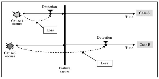
Figure 1.
Effect of failure-cause detection time on the loss of a failure: If a detection is later than a failure, the loss increases rapidly.
In this study, a time-dependent probabilistic approach is proposed considering the real situation that the loss increases as detection of a failure or its causes late, and the risk of the failure-cause is quantitatively evaluated based on this. Assuming a case function for detection time of a failure and its probable causes, an approximate loss function can be deduced for each failure-cause. Based on the value of the expected loss for each failure-cause, the risk priority metric (RPM) can be evaluated as the expected loss per unit time by multiplying the expected loss, which is determined by integration of loss function with its probability density function, and the occurrence rate of each failure-cause.
This manuscript has been organized as follows. Section 2 describes the proposed TD-FMEA model. In Section 3, a comparative analysis is conducted with the proposed TD-FMEA approach and traditional FMEA based on the design FMEA case of automotive leaf springs. Finally, we will draw conclusions and make suggestions for future research in Section 4.
2. Time-Dependent FMEA Model (TD-FMEA Model)
2.1. Modeling Procedure
The risk evaluation scheme of TD-FMEA proposed in this study is shown in Figure 2. First, probability density functions for occurrence time of failure , occurrence time of failure-cause , and detection time are defined. Next, the loss function is defined. For evaluating the expected loss, it must be set parameter values , , , , , and . By integrating the loss function, we deduce the expected loss . Finally, by multiplying the occurrence rate of failure-cause by , we get the expected loss per unit time (RPM) for a focused failure-cause.
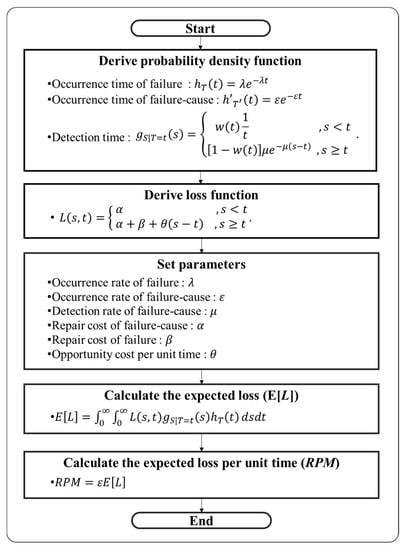
Figure 2.
Risk evaluation scheme of time dependent FMEA (TD-FMEA).
2.2. Risk Evaluation Modeling
Consider a random variable as an elapsed time from a failure-cause to the failure occurrence. Likewise, the detection time is defined by the elapsed time between a failure-cause and its detection. By defining an appropriate loss function as a function of the occurrence time and detection time , the expected loss can be calculated accurately. A typical failure scenario is depicted in Figure 1.
2.2.1. Occurrence Time of a Failure and Its Failure-Cause
Under the assumption of a homogeneous Poisson process (HPP), the occurrence time becomes a function of the failure occurrence rate . can be considered exponentially distributed with mean , and its probability density function is expressed as
Additionally, is defined by the occurrence time of the failure-cause from its operation. As in Equation (1), can be considered as a function of the failure-cause occurrence rate with its average value . The corresponding probability density and cumulative distribution functions are
2.2.2. Detection Time of a Failure-Cause
The probability density function of a corresponding failure-cause detection is generally assumed to be uniform before a failure occurrence, because a failure-cause is usually detected in accordance with the regularized detection schedule of a uniform time interval. Now, assume that we do not detect the failure-cause until the failure occurs. In the early stages of a failure, intensive detection will be attempted to detect failure-cause, so the probability density function of detection will be high at the initial state and will then gradually reduce. Thus, we considered an exponential function in this study, because it is the easiest to integrate and demonstrates excellent expansion. Therefore, probability density function of a failure-cause detection will be a case function conditioned by the time of occurrence.
Now, set up the following variables for obtaining the exact probability density function of detection time. Let us consider a failure and its failure-cause. Here, is the elapsed time between occurrence and detection of the failure-cause. Similarly, is the elapsed time between occurrence of failure and that of its failure-cause. As mentioned before, the conditional probability density function is uniform in the domain where a detection time is less than the given occurrence time . Otherwise, has an exponential form. Next, we have to determine the weight of the uniform and exponential section among the total probability 1. Let be the cumulative probability of the uniform distribution; then, is the cumulative probability of the exponential distribution as shown in Figure 3. Thus, the conditional probability density function is expressed as a function of the failure-cause detection rate , given the failure occurrence time .
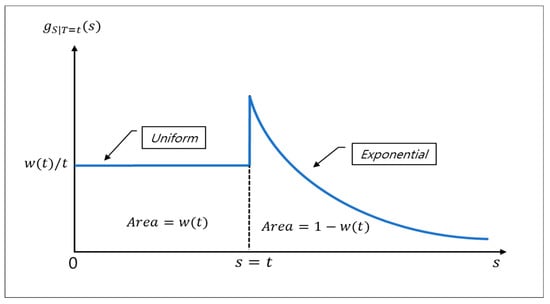
Figure 3.
Conditional probability density function of detection time , given of the failure occurrence time .
The function may jump up at . This is because more efforts are expected to be made to repair the failure and normalize the system at a time . Thus, for with jump up coefficient ,
Rearrangement of Equation (5) yields
The weight function equals zero when is zero and becomes unity as approaches infinity. This result is intuitively appropriate, since the probability of detection before failure would nearly equal zero when approaches zero, and as becomes infinitely large, the detection probability must approach unity. Thus,
2.2.3. Loss of Failure
If an inherent failure-cause exists within a system, there must be a cost associated with its elimination or prevention of the failure-cause. If a failure-cause is not detected until system failure occurs, it will add not only the failure-cause removal cost but also the system failure cost. The additional costs incurred as a result of system failure are the fixed cost and variable cost, i.e., a threshold cost and opportunity cost for system non-operation due to the system failure. The opportunity cost depends on the difference between failure-cause detection time and failure occurrence time . Let be a loss function for a system with several failure-cause. As we mentioned above, the loss is only the failure-cause removal cost for . However, for , the loss is the sum of a failure-cause removal cost, threshold cost of the system failure, and an opportunity cost of the system non-operation proportional to . That is,
Here, , and denotes a failure-cause removal cost, threshold cost of the system failure, and proportional factor of opportunity cost because of the system non-operation.
2.3. Loss Evaluation
2.3.1. Expected Value of Loss
The expected value of the loss function is calculated by integrating the loss function. From Equations (1), (4), and (8), the probability density function of failure occurrence time , failure-cause detection time , and the loss function are easily multiplied. Then, the expected value of the loss is calculated by the following.
(See Appendix A)
For , is the exponential integral function defined by
where is an irrational number called the Euler constant.
2.3.2. Risk-Prioritization Metric
Consider an occurrence of failure and failure-cause in a system. Suppose that a failure-cause of the failure occurs according to a homogeneous Poisson process (HPP) with a failure-cause occurrence rate . This statement is in fact equivalent to Equation (2). Finally, we propose the RPM compared with the RPN in the representative standard of FMEA. The is easily calculated by
3. Application
3.1. Parameters Setting of RPM and RPN Values
FMEA of product design, performed by Santhosh and Vinodh [4] for an organization that manufactures automotive leaf springs, was adopted in this research as a case study to demonstrate the utility of the proposed TD-FMEA model. Table 1 describes the FMEA chart for design documented as part of this case study. The modified chart describes analysis of various failure causes—from FC11 to FC23—listed under column 1 with O, S, and D. Numerical values were assigned to parameters , and , or simulations of the TD-FMEA model for design FMEA. A few of these parameter values were slightly modified as necessary to suit the proposed model. Values concerning the detection and occurrence rates— and —were obtained by modifying the corresponding ratings of factors O and D, respectively, in accordance with Table 2, which in turn, was modified with reference to the FMEA handbook [30].

Table 1.
Parameter setting for simulations of the time dependent FMEA (TD-FMEA) model for design FMEA: As shown in Equation (11), there are many parameters such as failure-cause detection rate , failure-cause occurrence rate , failure occurrence rate and coefficients , and of loss function . We set the parameters to compare risk prioritization metric (RPM) and risk prioritization number (RPN) by various simulations, fixing, and modifying each parameter.
Table 2.
Standardization of parameters for failure-cause occurrence rate , failure occurrence rate , and failure-cause detection rate : The guideline is referenced by Ford Motor Company [30].
In Table 2, occurrence rate of failure-cause and failure mode— and —for RPM are set to satisfy the given guideline such that cumulative probability of failure occurrence during unit time for the exponential distribution can be determined. Moreover, detection rate— for RPM is 1 over square-root of . This is because the effect of is opposite to that of , and is related to inspection policy compared to as an inherent property of the system. So, it assumes that the does not have dramatic range compared to . Parameters concerning the coefficient loss function—, and —were randomly assigned with reference to the S (severity) value of first column in Table 1. For parameters , and fixed and variable parameters were allocated to derive various simulation results.
3.2. Comparative Analysis of RPM and RPN
To illustrate the effectiveness of the proposed risk-evaluation technique, the above-described case study was used to analyze and compare results obtained using the proposed TD-FMEA model and conventional design FMEA techniques. The results are described in Table 3, that lists values of the conventional RPN, proposed RPM, and E[L] for each probable failure-cause in terms of both score and priority. To facilitate the robust evaluation of risks during the case study, results obtained for four cases ((a)–(d)) have been discussed herein considering, in each case, the effect of variation in the value of any one parameter among and . Figure 4 shows the correlation of priority of RPN and RPM in Table 3, respectively, in four cases. The square root of is 0.8 or higher, it is determined that there is a strong correlation [31]. The square root of always satisfies , the positive correlation is , the negative correlation is . Moreover, when it is free, it becomes .
Table 3.
Comparison between RPN of conventional FMEA model and RPM of TD-FMEA model for design FMEA: The priority of RPN and RPM is similar, so we may confirm the validity of the TD-FMEA model to some extent. (※ set and to the modified values in Table 1).
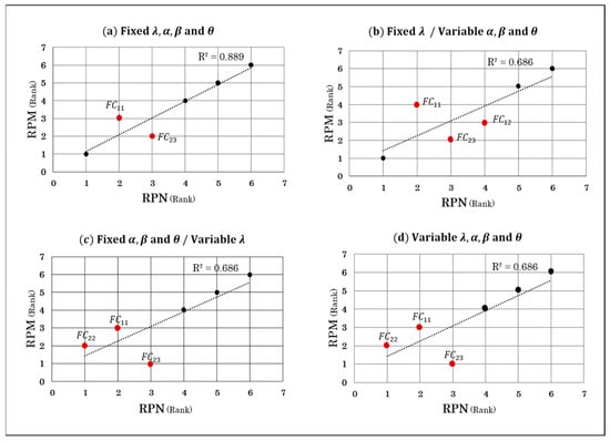
Figure 4.
Rank correlation between RPM and RPN obtained by design FMEA: RPM and RPN are strongly correlated except for slight variations in priority rank. In this case, square root of is Spearman correlation coefficient, i.e., Pearson correlation coefficient of rank.
In Figure 4, regarding case (a), the square root of between RPN and RPM was 0.943, indicating a strong correlation. In Table 3, however, in terms of score, they are different. Based on RPN values, the FC22 () demonstrates the highest priority and can be considered the most critical risk closely followed by FC11 (score = 210) and FC23 (score = 192) ranked second and third, respectively. The difference in RPN scores corresponding to the FC22 and FC11 is 30 (= 240 − 210), whereas that between the FC11 and FC23 is 18 (210 − 192). This, however, does not imply that 30 equals two times 18 from the viewpoint of risk size. In the case of RPM, the FC22 (score = 401) demonstrates the highest priority and can be considered the most critical risk followed by FC23 (score = 182) and FC11 (score = 22) ranked second and third, respectively. The difference in score corresponding to the FC22 and FC23 is 219 (401 − 182), whereas that between the FC23 and FC11 is 160 (182 – 22). This means that 219 is about 1.37 times larger 160 from the viewpoint of risk size. Moreover, as depicted in Figure 4 for case (a), the FC11 and FC23 are prioritized as three and two, respectively, when employing the RPM-based approach, whereas the same failure-causes are prioritized as two and three, respectively, in accordance with RPN values. This is because the occurrence rate for the FC23 is considerably higher compared to that for FC11, although the parameter is not significantly different for both risks (refer Table 1). This result is also reflected in RPM scores corresponding to the two cases. The score corresponding to the FC23 (score = 182) equals eight times that corresponding to FC11 (score = 22); that is, the loss incurred per hour in the event of a failure-caused by FC23 would be eight times that incurred in the event of a failure that was caused by FC11. On the other hand, this result is different in terms of . As described in Table 3, the FC23 with = 945 assumes the least priority. This implies that there is a high probability of detecting the FC23 before the failure occurs; thus, its corresponding score is low.
Regarding case (b), in Table 3, FC22, FC13, and FC21 are consistently assigned priorities of 1, 5, and 6, respectively, using both the RPN- and RPM-based approaches. As depicted in Figure 4 for case (b), the square root of between RPN and RPM was 0.829, indicating a strong correlation. Additionally, the FC11, FC23, and FC12 are assigned of 4 (score = 23), 2 (score = 428), and 3 (score = 29), respectively, when employing the RPM-based approach, whereas the same failure-causes are prioritized as two (score = 210), 3 (score = 192), and 4 (score = 168), respectively, when employing the RPN-based approach. This is because, as described in Table 1, variable parameters and for FC23 and FC12 exceed those for fixed parameters. On the other hand, in terms of , the FC11 with the smallest value of parameter assumes the highest priority, whereas risk FC12 with the largest values of assumes the lowest priority (refer Table 1).
In case (c), compared to RPM-based results obtained for case (a) (refer Figure 4), it can be realized that the RPM-based priority assigned to the FC22 changes from one to two while that of the FC23 changes from two to one. This is because the value of parameter for the FC23 exceeds that for the FC22 by a fairly large magnitude (refer Table 1). In contrast, in terms of , the FC11 with medium value of and the smallest value of assumes the highest priority, whereas the FC22 with small value of and large value of is assigned the lowest priority.
Lastly, in case (d), compared to RPM-based results, for case (d) are identical to those obtained for case (c) in terms of priority, and they are quite similar on the score side. In Figure 4, the square root of between RPN and RPM was also 0.829, indicating a strong correlation. On the other hand, in terms of , results are quite different. For example, for the FC13, the score of is more than double in case (d) than in case (c). This is because the and increased at the same time for case (d) (refer Table 3).
In most cases, the rankings cannot be fully matched because the method of derivation of RPN and RPM is completely different. Since RPN is not a perfect risk measurement tool currently, it is difficult to distinguish the superiority of RPN and RPM for the difference in rank. However, since correlation coefficients are high enough (higher than 0.8 for most cases), it is hard to say that RPN and RPM make a significant difference. RPM means the size of risk or loss unlike RPN, so RPM may have a wider range of applications than RPN. Above all, the parameters O, S, and D of RPN have over-dependence on expert intuition and experience instead of scientific methods for evaluation. However, the parameters of RPM are derived from statistical inference () and cost analysis (). Thus, we may say the RPM measured by TD-FMEA model is more objective than RPN evaluated by the conventional FMEA model.
4. Conclusions
So far, we have proposed a time-dependent FMEA model (TD-FMEA model) and obtained an expected loss value according to the occurrence of failure-cause through accurate calculation (Equation (9)). Then, we derived risk prioritization metric (RPM), which is a defined index measuring the risk of failure-cause in this study, multiplying by the failure-cause occurrence rate and the expected loss value (Equation (11)).
The mathematical model proposed in this study performs an associated calculation on system failure, failure-cause, and its detection. The probability density function of failure and failure-cause are exponential by homogeneous Poisson process (HPP) assumption (Equations (1) and (2)), and that of failure-cause detection is a case function combined in a uniform and exponential manner (Equation (4)). The loss function is also a case function conditioned by detection time of failure-cause and occurrence time of failure (Equation (8)). Time-dependent probabilistic approach pursues logical improvement compared to previous models. Conventional RPN approach assumes that O (occurrence of failure), S (severity of failure), and D (detection of failure-cause) are independent. However, RPM in our model does not assume the independence because it combines failure occurrence rate, detection rate of failure-cause, and loss function to derive the risk of failure-cause. Table 4 compared the traditional FMEA and our TD-FMEA model.
Table 4.
Comparison of traditional FMEA and TD-FMEA.
The RPM derived in this way provides room to supplement the disadvantages of traditional risk prioritization number (RPN). The coefficient of determination between the priority of RPM and RPN has a range of 0.686~0.889 in our example (Figure 4). That is the rank correlation has a range of 0.828~0.943, so that RPM and RPN have very strong correlations. From this, we can say that the validity of our model has been empirically proven. Furthermore, our model has the advantage that the RPM value represents the relative size of the actual risk. In contrast, the product of O, S, and D derived from RPN of conventional approaches is only an auxiliary value to derive the priority without having any substantial meaning (Table 3). Utility of both indicators and RPM with regard to evaluation of the risk associated with each failure has been described in great detail in Section 3 of this paper. For a reasonable calculation, we provide a standardization of parameters for failure-cause occurrence rate , failure occurrence rate , and failure-cause detection rate , which is a variation of our model from the guideline of Ford Motor Company (Table 2). In addition, the results of the sensitivity analysis of RPM can be found in Appendix B.
In future endeavors, our future prospect is to examine actual cases based on actual parameters. The purpose of the study is to derive correlation coefficients of RPN and RPM rankings to infer the validity of RPM, and to verify the effectiveness by deriving risks from RPM values. Moreover, we intend to focus on development of an FMEA risk-assessment methodology for a single failure with multiple causes along with determination of an optimal inspection period to enhance the detection rate based on values. In addition, if the failure-causes are analyzed hierarchically, a time-dependent probabilistic model will be developed based on undetected time.
- (i)
- In traditional FMEAs, risks can be assessed on a ranking basis, making it an easy-to-use approach when data is difficult to obtain. In the big data world, however, the application of a numerical-based TD-FMEA approach will enable more accurate assessment of risk.
- (ii)
- In traditional FMEAs, the results of a risk assessment may depend on the subjective opinion of the expert. On the other hand, in the case of the TD-FMEA approach, the objectivity of the result is secured based on probability.
Author Contributions
Conceptualization, H.-a.J. and S.M.; Methodology, H.-a.J. and S.M.; Modeling, S.M.; Validation H.-a.J. and S.M.; Writing—original draft preparation, H.-a.J. and S.M.; Writing—Review and Editing, H.-a.J.; and S.M.; Funding Acquisition, H.-a.J. and S.M.
Funding
This work was supported by the National Research Foundation of Korea (NRF) in a grant funded by the Korean government (MSIT) (No. 2019R1G1A1010335 and 2017R1C1B5017491).
Conflicts of Interest
The authors declare no conflict of interest.
Appendix A
For , is the exponential integral function defined by
where is an irrational number called the Euler constant. Therefore,
Appendix B
A sensitivity analysis was performed in this study to investigate the influence of distribution-parameter values on those of RPM. Sensitivity of RPM values to values of parameters— and —can be readily analyzed. In this study, sensitivity of the value of RPM was analyzed by assigning parameters , , and with constant of 1.81E−02, 200, 1000, and 1200, respectively. Variations in the value of RPM corresponding to changes in values of and are listed in Table A1 and depicted in Figure A1, respectively. Results obtained demonstrate that smaller values of result in enhanced sensitivity of RPM. Figure A1a demonstrates that the value of RPM steeply increases with reduction in the value of . Secondly, as depicted in Figure A1b, it can be realized that the value of RPM is nearly insensitive to small values of , and that the corresponding sensitivity increases with increase in the value of .
Figure A1 demonstrates that the maximum value of RPM is realized for the case wherein and . This implies that maximization of a given risk of failure with the corresponding failure-cause is hardly detectable whilst having a high occurrence probability. As depicted in Figure A1, there exists a big difference between RPM values obtained for each . This can be verified in terms of the graph slope. In Figure A1a, the difference between RPM values is large for cases with and assuming values in the range of 2–7. On the other hand, the difference between RPM values is small when and assumes values in the range of 1–6. This implies that the RPM value does not demonstrate much difference when the failure probability is either very high or very low. Inferences drawn from the above sensitivity analysis are that (i) each failure-cause with a high occurrence probability must be taken care of; and (ii) a cause with a small occurrence probability need not be assigned high priority.
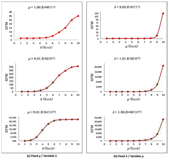
Figure A1.
Risk-prioritization metric (RPM) graph with respect to the failure occurrence rate and failure-cause detection rate (, , , , and ). (a) RPM as a function of draws S-curve, and (b) RPM of increases rapidly more than exponential. Thus, the RPM is more sensitive to than .
Table A1.
Risk-prioritization metric (RPM) table with respect to the failure occurrence rate and failure-cause detection rate (, , , , and ).
Table A1.
Risk-prioritization metric (RPM) table with respect to the failure occurrence rate and failure-cause detection rate (, , , , and ).
| 1st | 2nd | 3rd | 4th | 5th | 6th | 7th | 8th | 9th | 10th | ||
|---|---|---|---|---|---|---|---|---|---|---|---|
| 1.00∙E+00 | 7.65∙E−01 | 4.39∙E−01 | 2.72∙E−01 | 1.35∙E−01 | 6.01∙E−02 | 2.69∙E−02 | 9.81∙E−03 | 3.10∙E−03 | 9.81∙E−04 | ||
| 1st | 9.62∙E−07 | 3.6 | 3.6 | 3.6 | 3.6 | 3.6 | 3.7 | 3.9 | 5.2 | 17.6 | 122.3 |
| 2nd | 9.62∙E−06 | 3.6 | 3.6 | 3.6 | 3.7 | 3.7 | 4.1 | 5.5 | 15.6 | 101.8 | 779.1 |
| 3rd | 9.62∙E−05 | 3.7 | 3.7 | 3.7 | 3.8 | 4.4 | 6.7 | 16.6 | 81.7 | 582.8 | 3957.5 |
| 4th | 7.22∙E−04 | 3.8 | 3.9 | 4.2 | 4.8 | 7.5 | 19.1 | 65.1 | 335.4 | 2070.7 | 11,132.7 |
| 5th | 3.61∙E−03 | 4.3 | 4.5 | 5.7 | 8.0 | 17.0 | 53.0 | 182.3 | 833.3 | 4159.8 | 17,546.2 |
| 6th | 1.81∙E−02 | 5.9 | 6.8 | 10.5 | 17.3 | 42.4 | 131.6 | 405.0 | 1519.6 | 5981.7 | 20,942.4 |
| 7th | 7.40∙E−02 | 9.6 | 11.9 | 20.3 | 34.9 | 83.5 | 232.4 | 621.3 | 1965.1 | 6720.4 | 21,883.9 |
| 8th | 1.93∙E−01 | 14.2 | 17.9 | 30.9 | 52.1 | 116.8 | 296.2 | 725.7 | 2119.6 | 6912.5 | 22,092.6 |
| 9th | 5.85∙E−01 | 21.9 | 27.3 | 45.4 | 72.7 | 149.7 | 345.8 | 791.1 | 2198.9 | 6999.4 | 22,182.3 |
| 10th | 1.00∙E+00 | 26.0 | 32.2 | 52.0 | 81.1 | 160.9 | 360.0 | 807.3 | 2216.5 | 7017.6 | 22,204.6 |
References
- Stamatis, D.H. Failure Mode and Effect Analysis: FMEA from Theory to Execution, 2nd ed.; ASQ Quality Press: Milwaukee, WI, USA, 1995. [Google Scholar]
- Liu, H.; Liu, L.; Liu, N. Risk evaluation approaches in failure mode and effects analysis: A literature review. Expert Syst. Appl. 2013, 40, 828–838. [Google Scholar] [CrossRef]
- Geum, Y.; Cho, Y.; Park, Y. A systematic approach for diagnosing service failure: Service-specific FMEA and grey relational analysis approach. Math. Comput. Model. 2011, 54, 3126–3142. [Google Scholar] [CrossRef]
- Santhosh, D.; Vinodh, S. Application of FMEA to an automotive leaf spring manufacturing organization. TQM J. 2012, 24, 260–274. [Google Scholar]
- Yazdi, M.; Daneshvar, S.; Setareh, H. An extension to Fuzzy Developed Failure Mode and Effects Analysis (FDFMEA) application for aircraft landing system. Saf. Sci. 2017, 98, 113–123. [Google Scholar] [CrossRef]
- Wang, W.; Liu, X.; Qin, Y.; Fu, Y. A risk evaluation and prioritization method for FMEA with prospect theory and Choquet integral. Saf. Sci. 2018, 110, 152–163. [Google Scholar] [CrossRef]
- Fattahi, R.; Khalilzadeh, M. Risk evaluation using a novel hybrid method based on FMEA, extended MULTIMOORA, and AHP methods under fuzzy environment. Saf. Sci. 2018, 102, 290–300. [Google Scholar] [CrossRef]
- Mentes, A.; Ozen, E. A hybrid risk analysis method for a yacht fuel system safety. Saf. Sci. 2015, 79, 94–104. [Google Scholar] [CrossRef]
- Zhou, Q.; Thai, V.V. Fuzzy and grey theories in failure mode and effect analysis for tanker equipment failure prediction. Saf. Sci. 2016, 83, 74–79. [Google Scholar] [CrossRef]
- Maniram Kumar, A.; Rajakarunakaran, S.; Pitchipoo, P.; Vimalesan, R. Fuzzy based risk prioritisation in an auto LPG dispensing station. Saf. Sci. 2018, 101, 231–247. [Google Scholar] [CrossRef]
- Rhee, S.J.; Ishii, K. Using cost based FMEA to enhance reliability and serviceability. Adv. Eng. Inform. 2003, 17, 179–188. [Google Scholar] [CrossRef]
- Dong, C. Failure mode and effects analysis based on fuzzy utility cost estimation. Int. J. Qual. Reliab. Manag. 2007, 24, 958–971. [Google Scholar] [CrossRef]
- Von Ahsen, A. Cost-oriented failure mode and effects analysis. Int. J. Qual. Reliab. Manag. 2008, 25, 466–476. [Google Scholar] [CrossRef]
- Parracho Sant’Anna, A. Probabilistic priority numbers for failure modes and effects analysis. Int. J. Qual. Reliab. Manag. 2012, 29, 349–362. [Google Scholar] [CrossRef]
- Certa, A.; Hopps, F.; Inghilleri, R.; La Fata, C.M. A Dempster-Shafer Theory-based approach to the Failure Mode, Effects and Criticality Analysis (FMECA) under epistemic uncertainty: Application to the propulsion system of a fishing vessel. Reliab. Eng. Syst. Saf. 2017, 159, 69–79. [Google Scholar] [CrossRef]
- Huang, J.; Li, Z.; Liu, H. New approach for failure mode and effect analysis using linguistic distribution assessments and TODIM method. Reliab. Eng. Syst. Saf. 2017, 167, 302–309. [Google Scholar] [CrossRef]
- Catelani, M.; Ciani, L.; Venzi, M. Failure modes, mechanisms and effect analysis on temperature redundant sensor stage. Reliab. Eng. Syst. Saf. 2018, 180, 425–433. [Google Scholar] [CrossRef]
- Kim, K.O.; Zuo, M.J. General model for the risk priority number in failure mode and effects analysis. Reliab. Eng. Syst. Saf. 2018, 169, 321–329. [Google Scholar] [CrossRef]
- Ding, X.; Su, Q.; You, J.; Liu, H. Improving risk evaluation in FMEA with a hybrid multiple criteria decision making method. Int. J. Qual. Reliab. Manag. 2015, 32, 763–782. [Google Scholar]
- Mohsen, O.; Fereshteh, N. An extended VIKOR method based on entropy measure for the failure modes risk assessment—A case study of the geothermal power plant (GPP). Saf. Sci. 2017, 92, 160–172. [Google Scholar] [CrossRef]
- Lo, H.; Liou, J.J.H.; Huang, C.; Chuang, Y. A novel failure mode and effect analysis model for machine tool risk analysis. Reliab. Eng. Syst. Saf. 2019, 183, 173–183. [Google Scholar] [CrossRef]
- Yousefi, S.; Alizadeh, A.; Hayati, J.; Baghery, M. HSE risk prioritization using robust DEA-FMEA approach with undesirable outputs: A study of automotive parts industry in Iran. Saf. Sci. 2018, 102, 144–158. [Google Scholar] [CrossRef]
- Sharma, R.K.; Sharma, P. System failure behavior and maintenance decision making using, RCA, FMEA and FM. J. Qual. Maint. Eng. 2010, 16, 64–88. [Google Scholar] [CrossRef]
- Guimarães, A.C.F.; Lapa, C.M.F.; Moreira, M.D.L. Fuzzy methodology applied to Probabilistic Safety Assessment for digital system in nuclear power plants. Nucl. Eng. Des. 2011, 241, 3967–3976. [Google Scholar] [CrossRef]
- Pillay, A.; Wang, J. Modified failure mode and effects analysis using approximate reasoning. Reliab. Eng. Syst. Saf. 2003, 79, 69–85. [Google Scholar] [CrossRef]
- Carmignani, G. An integrated structural framework to cost-based FMECA: The priority-cost FMECA. Reliab. Eng. Syst. Saf. 2009, 94, 861–871. [Google Scholar] [CrossRef]
- Zammori, F.; Gabbrielli, R. ANP/RPN: A Multi Criteria Evaluation of the Risk Priority Number. Qual. Reliab. Engng. Int. 2012, 28, 85–104. [Google Scholar] [CrossRef]
- Peeters, J.F.W.; Basten, R.J.I.; Tinga, T. Improving failure analysis efficiency by combining FTA and FMEA in a recursive manner. Reliab. Eng. Syst. Saf. 2018, 172, 36–44. [Google Scholar] [CrossRef]
- Jang, H.A.; Lee, M.K.; Hong, S.H.; Kwon, H.M. Risk Evaluation Based on the Hierarchical Time Delay Model in FMEA. J. Korean Soc. Qual. Manag. 2016, 44, 373–388. [Google Scholar] [CrossRef]
- Ford Design Institute. FMEA Hand Book Version 4.1; Ford Design Institute: Dearborn, MI, USA, 2004; p. 290. [Google Scholar]
- Evans, J.D. Straightforward Statistics for the Behavioral Sciences; Thomson Brooks/Cole Publishing Co.: Belmont, CA, USA, 1996. [Google Scholar]
© 2019 by the authors. Licensee MDPI, Basel, Switzerland. This article is an open access article distributed under the terms and conditions of the Creative Commons Attribution (CC BY) license (http://creativecommons.org/licenses/by/4.0/).