Featured Application
The intelligent path recognition approach based on KPCA(kernel principal component analysis)–BPNN(back-propagation neural network) and IPSO (improved particle swarm optimization)–BTGWP(binary tree guidance window partition) promises to be an effective tool for estimating the guide-path parameters accurately for a vision-based automated guided vehicle (AGV)running in a complex workspace, even if the actual path pixels is surrounded by many under- or over-segmentation error points, which are caused by the non-uniform illumination, sight-line occlusion or stripe damage interferences inevitably on the image segmentation stage of a low-cost vision guidance system.
Abstract
Applying computer vision to mobile robot navigation has been studied more than two decades. The most challenging problems for a vision-based AGV running in a complex workspace involve the non-uniform illumination, sight-line occlusion or stripe damage, which inevitably result in incomplete or deformed path images as well as many fake artifacts. Neither the fixed threshold methods nor the iterative optimal threshold methods can obtain a suitable threshold for the path images acquired on all conditions. It is still an open question to estimate the model parameters of guide paths accurately by distinguishing the actual path pixels from the under- or over- segmentation error points. Hence, an intelligent path recognition approach based on KPCA–BPNN and IPSO–BTGWP is proposed here, in order to resist the interferences from the complex workspace. Firstly, curvilinear paths were recognized from their straight counterparts by means of a path classifier based on KPCA–BPNN. Secondly, an approximation method based on BTGWP was developed for replacing the curve with a series of piecewise lines (a polyline path). Thirdly, a robust path estimation method based on IPSO was proposed to figure out the path parameters from a set of path pixels surrounded by noise points. Experimental results showed that our approach can effectively improve the accuracy and reliability of a low-cost vision-guidance system for AGVs in a complex workspace.
1. Introduction
Automated guided vehicles (AGV) are a typical industrial mobile robot used for repeating transportation tasks in factories for decades [1,2,3]. Applying computer vision to mobile robot navigation has been studied for more than two decades [4,5,6]. Although the well-known Kiva robot can visually recognize an array of bars or two-dimensional codes on the floor as landmarks [7], cameras are still not widely used for the vision guidance of commercial off-the-shelf (COTS) AGV products in the current industrial applications [8].
In order to convince industrial practitioners of the virtues of computer vision, a low-cost vision guidance system based on intelligent recognition and decision-making mechanisms was developed for an AGV operating in a complex flow network [9]. Moreover, Kelly [1] declared that their floor mosaic guidance system had achieved sufficient maturity tested in an auto assembly plant. However, system integrators and AGV end-users still hesitate to adopt the scientific advances to their industrial practice, questioning their accuracy, complexity, cost, and reliability.
It seems that scientific results published to date neither provide sufficient accuracy for industrial applications nor have they been extensively tested in realistic, industrial-like operating conditions [10]. In fact, the recognition performance of machine vision systems is susceptible to external environments, especially the surrounding illumination [11,12]. As mentioned by Garibotto in [6], future developments should concern how to improve the adaptability of the vision system to illumination changes, since the frame grabber gain and offset parameters in image processing have to be adjusted in the light of variable contrast conditions.
Some progress has been achieved in the field of dealing with illumination changes in vision navigation [13,14,15,16,17,18,19], e.g., a colour model that separated brightness from chromaticity for feature matches between images with dynamic light sources [14], an entropy minimization method in the log-chromaticity colour space for the estimation of illumination invariant road direction [16], a parallel-snake model for lane detection with broken boundaries [17], a multilayer perceptron learning the relation between lane colour and illumination condition [18], and an adaptive image illumination partitioning and threshold segmentation approach based on a model of illumination and colour [19]. However, these current methods still have some under- or over-segmentation problems that fail to distinguish path pixels from background pixels or vice versa when road surfaces consist of shadow and highlight regions at the same time.
If the path pixels are recognized correctly with few under- or over-segmentation errors, it is not difficult to obtain the path equation by means of model estimation methods. The points conforming to the parallel characteristics, the length and angle characteristics, and the intercept characteristics of lane lines are selected in Hough space and then directly converted into the lane line equation [20]. An effective lane detection method based on an improved Canny edge detector and least square fitting was proposed in [21].The dual-threshold selection of a traditional Canny detector was improved using the histogram concavity analysis, and the least square method was used to fit the feature points of detected edges to accurate and single-pixel wide lane. Tan [22] proposed an algorithm based on improved river flow and random sample consensus (RANSAC) for the detection of curve lanes under challenging conditions, including dashed lane markings and vehicle occlusion. RANSAC was used to calculate the curvature of curve lanes according to the feature points with noises, derived from the process of improved river flow. A new method based on a binary image pyramid and two different dimensional Hough transforms was developed to extract lines from the images with noise points [23]. The foregoing methods, i.e., the least square method, the RANSAC algorithm, and the Hough transform, can provide satisfactory recognition results under the ideal conditions of feature points without noises, while they tend to be sensitive to the interferences from the complex surrounding illumination.
In fact, if high-quality images can be obtained by means of cameras, image-based navigation methods will be used broadly for maritime, aerial, and terrestrial environments. In the framework of comparative navigation, or termed terrain reference navigation, the position can be plotted by comparing a dynamically acquired image with a pattern image, which may be a numeric radar, sonar or aerial charts [24,25]. Similarly, the nonlinear characteristics of a feature-based positioning sensor need to be handled for terrain reference navigation systems [26]. In this sense, the acquisition of the high-quality images is vital for vision navigation of mobile robots, which requires an accurate and reliable vision recognition system.
The motivation of this paper lies in improving the accuracy and reliability of vision recognition of guide paths for AGVs running in a complex circumstance, by means of artificial intelligence methods. An intelligent path recognition framework consisting of path classification, straight path estimation, and curvilinear path approximation is devised for vision guidance of AGVs. Our main contributions are three-fold: (1) An intelligent path classifier based on kernel principal component analysis (KPCA) and a back-propagation neural network (BPNN) is proposed for distinguishing curvilinear paths from straight paths in an image with noise points; (2) a curvilinear path approximation method based on binary tree guidance window partition (BTGWP) is developed for substituting a series of piecewise linear paths for curvilinear paths, in accordance with a given approximation accuracy; and (3) a resist-interference path estimation method based on improved particle swarm optimization (IPSO) is investigated to figure out the path parameters from a set of path pixels with many under- or over-segmentation error points.
The remainder of this paper is organized as follows. The path recognition problem for AGVs traveling in a complex illumination circumstance is formulated in Section 2. Feature extraction and path classification based on KPCA and BPNN is proposed in Section 3. A path measurement model and the straight path estimation method based on IPSO are investigated in Section 4. The curve approximation method based on BTGWP is developed in Section 5. Experimental results of path recognition are analyzed by comparing our approach with some previous methods in Section 6. Conclusions and recommendations for future research are given in Section 7.
2. Problem Formulation
Line tracking is a mostly prospective vision navigation approach used in industrial fields, since it promises to be real-time, precise, and reliable. On one hand, the computational load relevant to this kind of vision perception is mitigated by coding or learning the specific perceptual knowledge that is expected to be extracted from the environment. On the other hand, a guide line is a kind of geometrically simplest landmark for vision navigation, which is beneficial for improving the measurement accuracy and reliability. Moreover, gluing a line on the floor is less costly compared to laying down a wire under the ground, or setting up a set of retro reflectors for a laser guidance system. Further, route adaptation and plant reconfiguration are vastly simplified since only removing and gluing lines on the floor is needed. Hence, a line-tracking vision guidance system is considered here for AGVs.
2.1. Vision Guidance System
The low-cost vision guidance system consists of a consumer-grade camera and a digital signal processor (DSP). Specifically, the analog charge-coupled device (CCD) camera adopted here has a resolution of 480 × 640 pixels, and a set of LED lights surrounding the CCD lens. The installation way of the onboard camera on AGVs can be either looking down vertically or obliquely. Although the vertical installation way can probably avoid the interference from the surrounding illumination to the vision guidance system to some extent, it will reduce the field of view of the onboard camera for vision guidance of AGVs, thereby restricting its predictive control performance. In order to collect abundant guidance information in a larger field of view, the onboard camera is mounted in the front of an AGV, looking down obliquely at coloured stripes on the ground, as shown in Figure 1.The field of view is determined by the installation height h and the pitch angle γ of the onboard camera. The geometric parameters are calibrated before the vision guidance system is used.
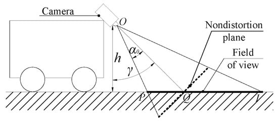
Figure 1.
The sketch of a vision-based automated guided vehicle(AGV).
Coloured stripes are set up on the floor as guide paths, which is the tracking target captured by the onboard camera in real time. The video signal is first generated in the phase alteration line (PAL) standard by the analog camera and then converted by a video decoder into an 8-bit YCbCrcolour digital image for the DSP. The texas instruments (TI) ® DSP DM642 is used as the image processor of vision guidance. The lateral position deviation and the orientation deviation of AGV are measured by the vision guidance system with respect to the given guide path. The workflow of the vision navigation system includes two stages: offline and online, as shown in Figure 2. The camera parameters are calibrated offline, then used online to rectify the image distortion and to convert the measurement unit from image pixel into physical dimensions, e.g., mm. Path pixel extraction can simply be regarded as an image operation of threshold segmentation, which divides the image into two regions: objects in the scene and the background, in terms of the difference of image threshold. The commonly used segmentation methods include the fixed single threshold, the fixed multiple threshold [20], the iterative optimal threshold, and the maximum inter-cluster variance (Otsu) [23]. Since under- or over-segmentation errors are unavoidable in the threshold segmentation for the current methods, path models have to be estimated according to a flock of target pixels with noise points. That is the main concern of this paper. Once the guide path is recognized from the background, two path deviations, i.e., the lateral position and orientation errors, can be calculated in the field of view of the onboard camera.
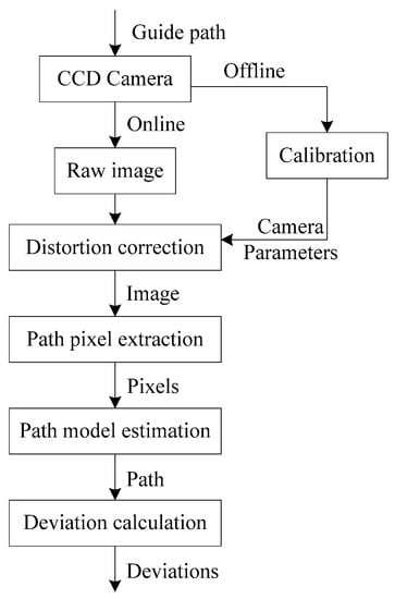
Figure 2.
The flowchart of line-tracking vision guidance.
2.2. Path Recognition Problem
Straight and curvilinear paths are mostly common in use for the line-tracking vision guidance of AGVs. If the path pixels are extracted correctly without being contaminated by a large amount of noise points, it is not a difficult task to estimate the path model by means of the least square method, the RANSAC algorithm or the Hough transform. Unfortunately, the aforementioned methods are vulnerable to the interferences caused by the non-uniform surrounding illumination when the onboard camera is set in the oblique installation way, or to the sight-line occlusion for the onboard camera due to some objects covering the path, or to stripe damage that obviously changes the previous appearance of the path because of wear and tear. In order to imitate these interferences occurring in the realistic industrial fields, a set of path images were sampled on the high-illumination condition, or contaminated using blue, red or white wastes, as shown in Figure 3.
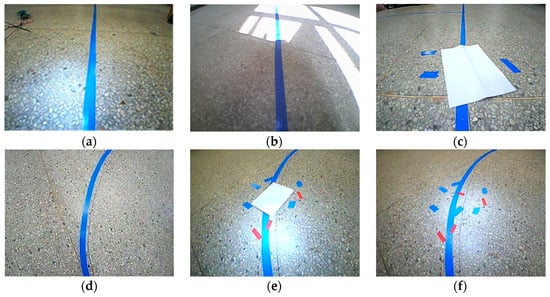
Figure 3.
Path images with interferences. (a) A straight path, (b) a straight path with highlights, (c) a straight path with coverings, (d) a curve path, (e) a curve path with highlights and coverings, and(f) a curve path with coverings.
Figure 3a,d shows the images collected for the straight and curvilinear paths on the normal illumination without any interference. Figure 3b,e was captured in a location with intense lighting, while Figure 3c,f shows the images of guide paths surrounded or overlapped by wastes. Either the non-uniform illumination or various wastes on the floor inevitably bring about the under- or over- segmentation problems in the threshold segmentation of path images. Hence, the model estimation approach is expected to be robust against these image noises. Particle swarm optimization (PSO) is a biomimetic approach imitating the predation behavior of birds, which is widely used for various multidimensional continuous space optimization problems based on particle swarm and fitness [27]. A segment-adjusting-and-merging optimizer is embedded into the genetic PSO evolutionary iterations to improve the search efficiency for the polygonal approximation problem [28]. PSO is also applied to compute an appropriate location of knots automatically for data fitting through B-splines, which is reported to be robust to noise points [29].
In fact, PSO is usually adopted as a parameter estimation approach for a known class of model. It implies that before PSO is used for the parameter estimation of guide paths, the class of path model, line or curve has to be recognized in advance. Hence, it is necessary to construct a robust path classifier to discriminate between a straight path and a curvilinear one. Usually, curvilinear paths are used for the turning operation of AGVs from one path to another, on which the relatively large deviations can be tolerated. In order to simplify the path model used in model estimation, a curvilinear path is approximated by means of piecewise straight lines. As a result, only the parameters of line model need to be solved.
2.3. Methodology Overview
For the guide paths existing with sight-line occlusion or stripe damage, under the complex illumination conditions, an intelligent path recognition approach based on KPCA–BPNN and IPSO–BTGWP was developed in order to suppress various interferences. The framework of this recognition approach is illustrated in Figure 4. A path classifier based on KPCA–BPNN was developed to differentiate a curvilinear path from a straight one, according to the geometric features. For the curvilinear paths, an approximation method based on BTGWP was developed for replacing the curve with a set of piecewise lines. The window size can be adjusted adaptively in the light of the radius of curvature and the accuracy of curve fitting. For the straight paths, the parameters of their path models were optimized based on IPSO, in order to make the path pixels surrounded by various noises accord with their model best. After the parameters of the path models were estimated, it was not difficult to calculate two path deviations of AGVs in the field of view.
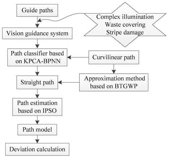
Figure 4.
The framework of path recognition based on KPCA (kernel principal component analysis)–BPNN (back-propagation neural network) and IPSO (improved particle swarm optimization)–BTGWP (binary tree guidance window partition).
3. Path Feature Recognition
The recognition process of path features includes threshold segmentation of path pixels, feature extraction of the path pixel set, and path model classification, as shown in Figure 5. The workflow of path feature recognition can be divided into two stages: offline training and online recognition. At the offline stage, the sample images of guide paths with various interferences of illumination, coverings, and damages are captured by the vision guidance system. The path pixels are extracted from the background with under- or over-segmentation error points in the YCbCr colour space by threshold segmentation, generating a piece of binary path image. A compound scanning technique of region projection and contour scanning is used to extract the path features from the binary image with noises. Both region projections in the directions of row and column, and four boundaries of the path contours, constitute a high-dimension feature vector for a path image. The feature vectors from a set of sample images comprise a feature matrix for the offline training of a classifier. In order to simplify the training process, principal component analysis was used to reduce the dimensionality of the feature vectors in the high-dimension kernel space (KPCA). Then, the dimension-reduced feature matrix was provided for the training of the classifier based on back-propagation neural network (BPNN). This classifier will have the generalization ability for new unknown path images, thereby being able to discriminate between straight paths and curvilinear ones at the online stage.
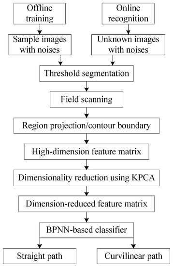
Figure 5.
The recognition process of path features.
3.1. Threshold Segmentation
Since the colour of guide paths is blue, the blue chrominance component Cb has an obvious contrast between the guide paths and the background in the YCbCr colour space, which is helpful for obtaining a better segmentation effect. Hence, the Cb component of path images was used as the raw data of path features. After the conversion of path images from the PAL standard to the YCbCr standard with a sampling ratio of 4:2:2, the resolution of the Cb component in path images is 480 × 360 pixels.
Path pixels can be identified by checking whether the Cb component of each pixel is larger than a threshold. If the path image is displayed in an invariant, uniform illumination circumstance, it is ready to determine the threshold that can separate the path from the background distinctly. Unfortunately, sometimes, the perceived colour of an object differs from its original colour, especially under non-uniform and dynamic illumination conditions.
Neither the fixed threshold methods nor the iterative optimal threshold methods can obtain a suitable threshold for all conditions. Even if some new colour models [14,16] or image enhancement methods [15] are reported to be able to separate chromaticity from brightness, a number of under- or over-segmentation error points remain around the actual path pixels. The possible path pixels are extracted with noise points from the original images in Figure 3 by means of the Otsu threshold segmentation method, as shown in Figure 6. Because of some objects covering the path, the binary image of path pixels is incomplete, with several parts missing. The non-uniform illumination interferes with the extraction of path pixels as well, e.g., the actual path becoming slender in the highlight regions, and some similarly narrow fake paths occurring beside it, as shown in Figure 6b.
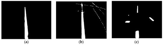
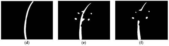
Figure 6.
The binary images of path pixels. (a) A straight path, (b) a straight path with highlights, (c) a straight path with coverings, (d) a curve path, (e) a curve path with highlights and coverings, and (f) a curve path with coverings.
3.2. Feature Extraction
In order to classify different types of guide paths with noise points, the path features were extracted using the field scanning technique [9]. The detailed field scanning process is described as follows.
(1) In the binary path image, assume the pixel value as f(x, y), where it is 1 for the path and 0 for the background.
(2) Scan all pixels in row j (1≤j≤N, N = 360) from left to right. Record the column coordinates of the first path pixel as hlj, that of the last path pixel as hrj, and the number of all path pixels as hpj.
(3) Scan all pixels in column i (1≤I≤M, M = 480) from top to bottom. Record the row coordinates of the first path pixel as vti, that of the last path pixel as vbi, and the number of all path pixels as vpi.
(4) The contour features of the path can be described by means of the four-boundary contour scanning. The corresponding feature vectors are:
(5) The region projections in the directions of row and column can be used for measuring the size features of the path. The feature vectors are:
(6) Insert one of the aforementioned feature vectors behind the end of another sequentially, to constitute a total feature vector P of a 3(M+N) dimension with redundant information, i.e.,:
In order to search the inherent characteristics in the high-dimensional observational data, the total feature vector P needs to be projected to a low-dimensional space [30]. First, the total feature vector P is mapped from its original space to a high-dimensional space H, i.e., the reproducing kernel Hilbert space [31], by means of a Gaussian radial basis kernel function. Then, kernel principal component analysis (KPCA) is used to reduce the dimensionality of feature vectors in the feature space [32]. The following steps are taken for dimensionality reduction.
(1) Collect n frames of path images as a training sample set for path features. Let the dimensionality of feature vectors be m = 3(M+N). These n feature vectors constitute a sample matrix Xn×m.
(2) An n×n real positive definite kernel function matrix K is developed for clustering data in the high-dimensional space H. The development process is as follows. Assuming the sample matrix:
, , where is the input space, and m is the dimension of the samples, xi, m = 3(M+N).
(3) The nonlinear mapping of the input space is X→H. Moreover, we assume that we are dealing with centered data, i.e., . Then, the covariance matrix C of the samples in the feature space H is:
(4) Assume that eigenvalues and eigenvectors both exist, which satisfy:
Then, all solutions V with lie in the span of .
Based on this finding, we can construct a group of equations, i.e.,:
There is certainly the possibility that a set of coefficients αi (i = 1, …, n) satisfy:
(5) Substitution of Equations (3) and (6) into Equation (5) yields:
Normally, the specific form of ϕ is unknown. Hence, the Gaussian radial basis kernel function к is employed as a replacement, where K is the kernel function matrix related to к.
(6) Upon substituting Equation (8) into Equation (7), one obtains:
where α denotes the column vector containing entries. α1, …, αn.
Once the solutions of Equation (9) are found, the nonzero eigenvalue problem can be settled. Let denote the eigenvalues of K, i.e., the solutions nλ of Equation (9), and are the complete set of eigenvectors corresponding to the eigenvalues, with λp being the first nonzero eigenvalue. The eigenvalues λi and the eigenvectors of the matrix K can be solved using the Jacobi iteration method [33].
(7) In order to extract the principal components, the projections of the samples onto eigenvectors Vk (k = p,…,n) in the feature space H need to be calculated. Let x be a new sample, with an image φ(x) in the space H. Then, the projections are the nonlinear principal components of the sample, shown as:
where hk(x) is the kth nonlinear principal component of the sample x.
(8) The contribution rate of the principal components is evaluated. Select s principal components whose rate of contribution is the most important, and whose sum of contribution is greater than 85%. Then, a new sample matrix with a reduced size of n×s is generated as an input when the BPNN-based classifier is trained.
3.3. Path Classification
The inherent mechanism of the back-propagation neural network is to propagate the error between the actual output value and the target value from the output layer of the network back to the input layer. At each layer, the neural network corrects the connection weights among neurons and the thresholds of each neuron, based on the error transmitted from the outer layer. The correction process is repeated continuously until the error has been converged to an acceptable level, or the operation of the algorithm reaches a maximum iteration steps preset.
The structure of a 3-layer BP neural network with a single hidden layer is adopted in this paper. Theoretically, this network can implement any nonlinear mapping with arbitrary precision. The number of the input nodes of the BPNN is the dimensionality s of the samples after the reduction by the KPCA. The sigmoid function is selected as the transfer function for the hidden layer. Since each group of samples corresponds to one path type, the number of the output nodes is defined as 1. The number of the hidden-layer nodes is determined according to the empirical formula.
where s is the number of the input nodes, q is the number of the output nodes, and a is a constant between 1 and 10.
The traditional BP learning algorithm is sensitive to the learning rate. In order to deal with this drawback, the adaptive momentum BP learning algorithm is adopted here [34]. The learning rate is adaptively adjusted in the light of the local error surface during the training process, which makes the learning algorithm achieve a fast and still stable convergence. For the BPNN, the initial learning rate, the target error, and the maximum iteration steps are set as 0.05, 0.001, and 1000, respectively. Then, the samples after the KPCA dimensionality reduction are provided to train the BPNN. The BPNN trained can adaptively adjust the network weights for any new input data, thereby having strong self-learning and self-adaptive ability. Moreover, this network also has some fault-tolerant capability, i.e., it can still work normally when the network is damaged partially.
4. Path Model Estimation
In a realistic industrial environment, both the non-uniform illumination and various wastes on the floor can cause the unavoidable under- or over-segmentation errors in the image segmentation process. For instance, when the possible path pixels are extracted from the original images in Figure 3 by means of the Otsu threshold segmentation method, a large number of noises and fakes appear beside the actual paths, or the paths recognized are incomplete and broken, as shown in Figure 6. The pixel fakes and path incompletion will influence the extraction of the center pixels of the path negatively, thereby degrading the estimation accuracy of the path model, as shown in Figure 7.
Figure 7.
The center pixels of the path images. (a) A straight path, (b) a straight path with highlights, (c) a straight path with coverings, (d) a curve path, (e) a curve path with highlights and coverings, and (f) a curve path with coverings.
Table 1 shows the statistical data of pixel classification for path images in Figure 7. The image pixels are classified into three types: black background pixels, white path pixels, and blue center pixels. The blue center pixels with noise points are recorded as the following set:

Table 1.
Pixel classification of path images.
In order to improve the recognition accuracy of the guide path, it is necessary to eliminate the effects of noise points and path incompletion on model estimation. Hence, IPSO is proposed to distinguish the actual path pixels from their fakes, obtaining an accurate straight path model, no matter what noise points and path incompletion occur.
4.1. Improved Particle Swarm Optimization
A number of particles which fly around in the search space to find the best solution are used in PSO [35,36,37,38]. Each particle denotes a candidate solution for optimization problems, which has two characteristics: position and velocity. Each position corresponds to a fitness value, calculated by the objective function. Each particle searches for the optimal solution in the solution space according to the fitness value. Moreover, it memorizes the current optimal solution at each step when the algorithm is iterated. The memory of each particle is updated by tracking two extrema. One is the best solution found by itself, called the individual extremum Pt. The other is the best solution that the swarm has obtained so far, called the global extremum Pg.
In the process of parameter estimation, the key operations of the genetic algorithm [39] include selection, crossover, and mutation, while PSO uses a real number coding method, without selection, crossover, and mutation, thereby having a simpler structure and a higher efficiency of calculation. However, conventional PSO is prone to falling into the local optimum and missing the global extremum [40,41]. In fact, the inertia weight of the algorithm reflects the ability of the particle to inherit the previous velocity at the current step. Shi [42] indicated that a large inertia weight is beneficial to the global search, while a smaller inertia weight is more favorable for the local search. In this sense, it is more advisable to update the inertia weight and acceleration factors and adaptively at each step, in order to take a tradeoff between the local search performance and the global search one. Hence, an IPSO algorithm is proposed here to avoid being trapped into the local optimum position.
4.2. Measurement Model
In order to formulate the measurement model, a measurement frame -o- was constructed in the field of view of the onboard camera, which is the image coordinate system for detecting the guide path, as shown in Figure 8. The image resolution is M×N. The installation orientation error of the camera is . The position of the optical center of the camera is J, which is also the vision measurement center of AGV. is the ideal angular deviation without considering the installation error . v(k) is the velocity of AGV. In this image coordinate system, the linear segment EI is a straight path. The distance between the optical center J and the straight path EI is defined as the lateral position deviation .
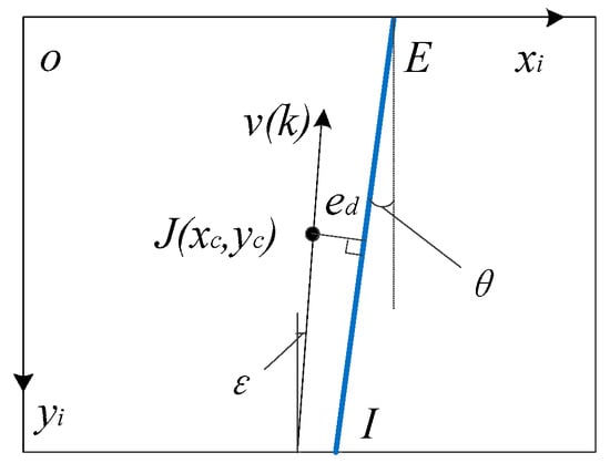
Figure 8.
Measurement model of a straight path.
If the straight path model is described by the equation in the image coordinate system, then the position deviation is calculated by:
The position deviation can then be converted into the world coordinate system, i.e.:
where is the factor to map from image pixel to physical dimension. The factor can be obtained by means of calibrating camera parameters.
In Figure 8, the actual orientation deviation considering is the angle between EI and v(k), which is:
For the blue center pixels of the guide path, the mean squared error for parameter estimation is:
How to choose the path parameters and in order to minimize the value of Equation (16) is essentially a nonlinear parameter estimation problem. It is solved by means of the following IPSO algorithm, which produces a parameter output of a straight path.
4.3. IPSO-Based Path Estimation
The detailed process of the IPSO-based path parameter estimation is shown in Figure 9, consisting of the following steps.
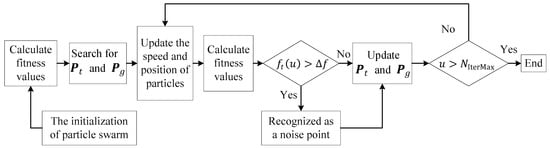
Figure 9.
IPSO-based path parameter estimation.
Step 1: Acquiring the path pixel set
Scan the binarized path image line by line, recording the pixel positions and of the left and right boundary points of the path. The blue center pixel set of the path is obtained.
Step 2: Defining the fitness function
Optimize the straight path parameters and based on the minimum mean squared error criterion. Equation (16) is defined as the fitness function of IPSO.
Step 3: Generating the particle swarm
In the h-dimensional parameter search space, the size of the particle swarm is r, i.e., r particles constitute the population . The tth particle is an h-dimensional vector, representing the position vector of the particle in the search space, i.e., , which is a potential solution for the parameter estimation problem. The velocity vector of the tth particle is . The velocity range of the particle swarm is [Vmin, Vmax], and its position range is [Qmin, Qmax].
Step 4: Initializing the particle swarm
The parameters of the particle swarm are configured as follows: the population size r = 20, and the maximum number of evolution generation NIterMax = 100. The first and last points of the target path center point set , i.e., and , are chosen to estimate the initial parameters of the straight path, obtaining and . Each individual of the particle swarm is initialized using the initial parameters, including the individual extremum Pt = [Pt1, Pt2,Pt3, …,Pth]T and the global extremum Pg = [Pg1, Pg2,Pg3, …, Pgh]T at the first each generation. The initial fitness value of each particle is calculated by means of Equation (16), used as the fitness value of the individual extremum and of the global extremum, i.e., and .
Step 5: Evolving the particle swarm
For the r particles in the uth generation (u = 1, 2, …, NIterMax), calculate the average value of all individual extrema by means of Equation(17):
The inertial weight of the tth particle is obtained by means of Equation (18):
Then, Equation (19) is used to compute the acceleration factor of the individual.
For the uth generation particle , calculate the dth (d = 1, 2, …, h) component of the velocity vector of the (u+1)th generation according to Equation (20).
where r1 and r2 are the random numbers uniformly distributed in the range of [0,1]. If Vtd(u+1) exceeds the speed range [Vmin, Vmax], adjust it to the nearest speed boundary value.
Moreover, Equation (21) is used to calculate the dth component of its position vector at the (u+1)th generation.
If exceeds the position range [Qmin, Qmax], adjust it to the nearest position boundary value. Then, the number of the evolutionary generations is increased by one, i.e., u = u + 1.
Step 6: Updating the particle swarm
The fitness value of the tth particle in the uth generation particle swarm is calculated by means of Equation (16). If the fitness value of the tth particle is better than that of its individual extremum, i.e., <, update the individual extremum and the fitness value of the tth particle, Pt= and = . If the fitness value of the tth particle is better than that of its global extremum, i.e., <, update the global extremum and its fitness value, Pg = and = .
Step 7: Identifying the noise points
Let the fitness threshold be . If the fitness value of the tth particle is greater than , the particle is identified as a noise point.
Step 8: Iterating the particle swarm
If the number of evolution generations u>NIterMax, stop evolving the particle swarm. The current global extremum Pg is given as the parameter output for the straight path model. Otherwise, go back to Step 5 to continue the evolution process of the particle swarm.
The IPSO-based path parameter estimation method is then utilized to further eliminate the influence of under- and over-segmentation errors occurring in the threshold segmentation stage. As shown in Figure 3b,c, the images of a straight path are exposed in the highlight or covered by some wastes. When the Otsu threshold segmentation method is used to extract the possible path pixels from these two original images, the under- and over-segmentation errors result in omitting target pixels or producing fake pixels, as shown in Figure 6b,c. Although the target paths in Figure 6b,c are incomplete and interfered by noise points, the IPSO method is able to distinguish the target points from the noise points, thereby estimating the genuine path correctly, as shown in Figure 10a,b.
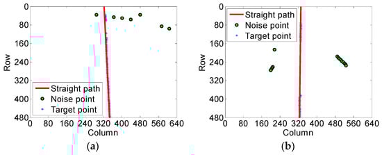
Figure 10.
The estimation results of the IPSO method for straight paths. (a) A straight path with highlights and (b) a straight path with coverings.
It is obvious that the IPSO-based path parameters estimation method is not sensitive to the noise points produced by the under- and over-segmentation errors in the threshold segmentation stage. The number of noise points and target points are listed in Table 2, which shows the high recognition accuracy for path pixels in the process of parameter estimation, discriminating between target points and noise ones. Hence, the straight path can be recognized precisely by the vision guidance system for AGVs in a complex workspace.
Table 2.
Recognition accuracy of a straight path with noise points.
5. Curvilinear Path Approximation
The guide paths tracked by an AGV may be straight or curvilinear. Usually, the operation points, e.g., loading and unloading workstations, are deployed on a straight path with high positioning accuracy. However, the curvilinear path is mostly used as the turning pathway to connect two adjacent straight paths. Hence, a relatively large guidance error can be tolerated when the AGV makes a turn on the curvilinear path. Moreover, a much simpler linear model is needed in the parameter estimation approach for the straight path, which has higher computational efficiency and stronger resist-interference performance, compared with the case for the curvilinear path. According to the principle of curve approximation in numerical control technology, a large number of small sections of basic lines (straight and circular) are considered to be able to approximate a complex irregular curve, as long as the step lengths of lines are small enough [43].
In order to make full use of the parameter estimation approach for the straight path, we propose a curvilinear path approximation method based on binary tree guidance window partition (BTGWP), which can convert a curvilinear path into a series of end-to-end connected straight paths, called a polyline path. The flowchart of the proposed method is shown in Figure 11. The method can automatically determine whether it is necessary to continue to partition the guidance window, based on the approximation error threshold predefined for the curvilinear path.
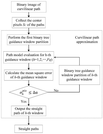
Figure 11.
The framework of binary tree guidance window partition.
Step 1: Acquiring the path image
Obtain the binarized image of a curvilinear path after the path recognition based on the KPCA–BPNN classifier. Make a contour scan on the binarized image, and then collect the center pixel set of the curvilinear path.
Step 2: Assuming a straight path model
Assume that the center pixel set pertains to a straight path. The linear model is used in the IPSO-based path parameter estimation approach for the center pixel set in the whole guidance window. The parameters of the straight path assumed are obtained, together with the output of the target points and the noise points.
Step 3: Calculating the mean squared error
Calculate the mean squared error of the distances that are measured from each target point of the set to the straight path estimated. Compare the mean squared error with the approximation error threshold .
Step 4: Partitioning the guidance window
If the mean squared error is less than or equal to the threshold , the straight path is the final estimation result. Otherwise, divide the guidance window into two subguidance windows equally. Then, go back to Step 2 and continue to estimate the straight path model for each subguidance window.
Taking the curvilinear path in Figure 12 as an example, we explain the specific implementation process of the BTGWP-based curvilinear path approximation method. In Figure 12, the blue points are the center pixel set , surrounded by some noise points. Arc AB is the ideal curvilinear guide path. Line segment A1B1 is the chord of arc AB. Line segment JG is the vertical line from the vision measurement center J to chord A1B1. Point T is the intersection point of line segment JG and curve AB. q(k) is the direction of the tangent line through point T on Arc AB.
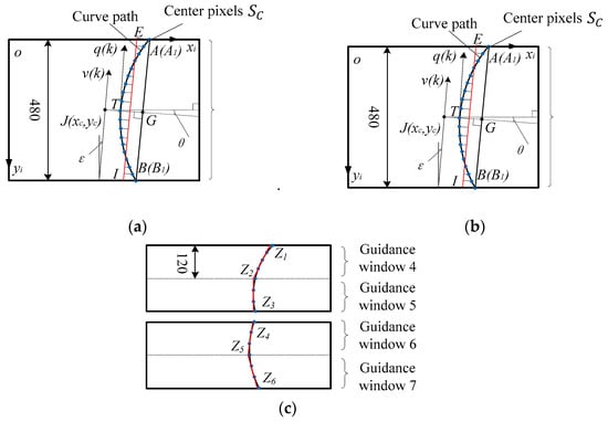
Figure 12.
The approximation process of curvilinear path. (a) The first estimation in the whole guidance window, (b) the second estimation in two subguidance windows, (c) the third estimation in four subguidance windows.
Firstly, a straight path model was estimated for the center pixel set in guidance window 1. The target points are distinguished from the noise points, where Snum is the number of target points, and SN1 are the target point set in guidance window 1. The straight path EI estimated is shown in Figure 12a, which can be expressed by the following formula: , where Fq is the number of guidance window partitions.
Secondly, the vertical distance vdi from each point of the set SN1 to the straight path EI is calculated by means of Equation (22). Then, Equation (23) is used to obtain the mean squared error of the vertical distance vdi in guidance window 1.
If , then the straight path EI is accepted as the approximation result for the curvilinear path AB. The BTGWP approximation method stops.
If , then the current guidance window is partitioned to two subguidance windows, e.g., guidance window 1 is divided into guidance windows 2 and 3, as shown in Figure 12b.
Thirdly, the IPSO-based path parameter estimation approach is again performed in guidance windows 2 and 3, respectively. The target point sets and are collected, with the corresponding straight path model E1T1 and T1I1 found, as shown in Figure 12b.
Fourthly, the mean squared errors and of the vertical distances in guidance windows 2 and 3 are calculated by means of Equations (22) and (23).
If and , then the straight paths straight paths E1T1 and T1I1 are the final approximation results for guidance windows 2 and 3.
If or , then guidance window 2 or 3 is equally divided into two subguidance windows, e.g., guidance windows 4 and 5 replace guidance window 2, as shown in Figure 12c.
The abovementioned process steps, i.e., the straight path model estimation, the mean squared error calculation, and the guidance window partition, are performed iteratively until the mean squared errors of each guidance window are all less than the threshold predefined. Finally, a polyline path, containing a series of end-to-end lines, is generated as an approximation result for the curvilinear path.
In terms of the operation requirements and the positioning accuracy in the industrial field, the radius of the curvilinear guide path and the approximation error threshold are preset as: R = 0.8 m and ∆α= 2 mm. The results of the curvilinear path approximation are shown in Figure 13. All mean squared errors are less than the threshold ∆α, as shown in Table 3. It is obvious that although a large number of noise points exist in the guide path image, the BTGWP approximation method can accurately convert an arbitrary curvilinear path into a polyline path, with high environmental adaptability and the curve approximation ability.
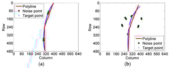
Figure 13.
Experiment results of curvilinear path approximation. (a) The curve path and (b) the curve path with highlights.
Table 3.
The approximation accuracy of the curvilinear path.
It is noteworthy that the threshold ∆α will affect the result of guidance window partition. For a curvilinear path with a 0.8 m radius, the relationship between the threshold Δα and the number Fq of guidance window partitions is modeled using a group of trials, as shown in Figure 14. A small threshold ∆α will increase the number of partitioning the guidance window. In this sense, it is convenient to change the curve approximation accuracy by adjusting the threshold ∆α dynamically.
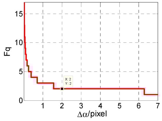
Figure 14.
The relationship between Fq and ∆α.
6. Experiments
A vision-guided differential-driving AGV prototype was developed, as shown in Figure 15, to verify the accuracy, real-time, and resist-interference performance of the intelligent path recognition based on KPCA–BPNN and IPSO–BTGWP. An obliquely looking-down CCD camera in the front of the vision-guided AGV was used to acquire the straight and curvilinear path images in the different operation fields. The Otsu threshold segmentation method was utilized to extract the possible path pixels from the original path images, which produces 100 experimental samples in total. The curvilinear paths were firstly discriminated from the straight paths in these sample data by means of the path classifier based on KPCA–BPNN. The IPSO-based estimation method was used to obtain the parameters of the straight paths. Each curvilinear path was converted into a polyline path, consisting of a series of end-to-end connected straight paths, which can then be solved using the similar IPSO-based method as the straight path. Since the linear model estimation methods are needed for both the straight path recognition and the curvilinear path approximation, our IPSO-based method was compared with the improved RANSAC (IRANSAC) algorithm [44], and the least squares (LS) method [45] in the experiment. The experiment system includes an industrial computer with a 2 GHz Intel Core i7-4510U processor and a 4 GB RAM at the hardware level, and a Matlab R2014a software on the Windows 8 operating system.
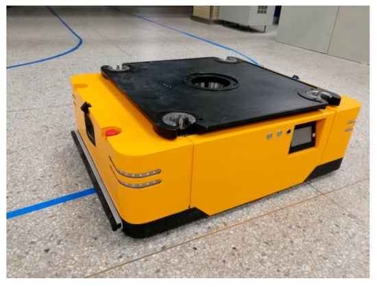
Figure 15.
The vision-guided AGV prototype.
The recognition rate and the average time consumption of the three methods are listed in Table 4. Since most experimental samples suffer from noise points, the model estimations of a straight path based on the IRANSAC and LS methods have obvious errors, making it impossible to identify the guide path correctly. Moreover, the real-time performance of the IPSO method is much better than that of the IRANSAC algorithm, i.e., the average time consumption is 61 versus 131.5 ms.
Table 4.
The performance comparison of three methods.
The fitting results of straight path based on the IPSO, IRANSAC, and LS methods are shown in Figure 16. The blue points are the raw data of the center pixel set . The red solid line is the estimation result for the straight path using the IPSO method, while the green dotted line and the yellow dashed line are the results based on the IRANSAC and LS methods, respectively. The parameters of the straight path model estimated using the three methods are listed in Table 5.
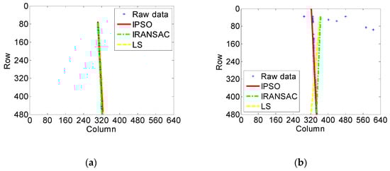
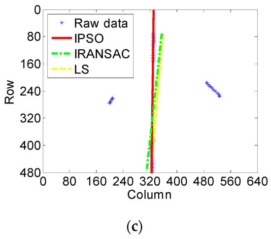
Figure 16.
The fitting results of a straight path using three methods: (a) a straight path, (b) a straight path with highlights, and (c) a straight path with coverings.
Table 5.
The parameters of straight paths.
If there are no or few noise points in the original path images, the Otsu threshold segmentation method can extract the center pixel set correctly. In this case, the three estimation methods can all recognize the straight path by fitting the center pixels, with similar recognition accuracy, as shown in Figure 16a.
If the original path images are disturbed by the complex illumination, sight-line occlusion or stripe damage, the center pixel set obtained by the Otsu threshold segmentation inevitably contains many noise points. In this case, the IPSO method still preserves high recognition accuracy for the straight path, while the recognition performance of the IRANSAC and LS methods deteriorates rapidly. Due to the distraction by the noise points, the model parameters estimated by the latter two methods deviate from the actual guide path significantly, as shown in Figure 16b,c.
In order to further illustrate the advantages of the IPSO method used for the model estimation of the straight path, the variation curves of the model parameters and , and the fitness value of the global extremum of the IPSO method are depicted in the 100 iteration evolution, as shown in Figure 17.
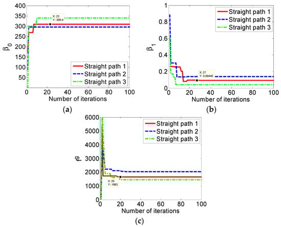
Figure 17.
The curve of particle swarm optimization (PSO)-based path model estimation. (a) The optimization process of parameter , (b) the optimization process of parameter , and (c) the optimization process of fitness value .
The parameter estimation process of straight path 1 in Figure 3a achieves convergence after 20 iterations, as shown in Figure 17. The fitness value of the global extremum is 1663, as shown in Figure 17c, with the corresponding particle position at point (309.40, 0.0943), as shown in Figure 17a,b.
The parameters of straight path 2 in Figure 3b are estimated as (295.30, 0.1382) after 25 iterations, with a 2046 fitness value. Similarly, the straight path 3 in Figure 3c is recognized after 20 iterations, the fitness value equaling to 1460 and the model parameters being (340.20, 0.0414).
The experimental results show that no matter whether the path images are interfered by the non-uniform illumination, sight-line occlusion or stripe damage, or no matter whether the path pixels are surrounded by the under- or over-segmentation error points, the IPSO method we propose is able to estimate an accurate linear model for the straight path by recognizing the actual path pixels from their image artifacts.
7. Conclusions
Earlyadopters who attempt to explore the feasibility of applying computer vision to mobile robot navigation are still confronted with many difficulties. The most challenging problems for a vision-based AGV running in a complex workspace involve non-uniform illumination, sight-line occlusion or stripe damage, which inevitably result in incomplete or deformed path images as well as many fake artifacts. An intelligent path recognition approach based on KPCA–BPNN and IPSO–BTGWP is proposed in this paper, which can convert a curvilinear path into a piecewise straight paths first and then estimate an accurate linear model for each straight line, no matter what kind of the under- or over-segmentation error points occur in the preprocessing stage of image segmentation. Experimental results show that our approach has a high robustness performance to resist the interferences from the complex workspace in which the AGV operates. In future research work, a low-cost vision guidance system will be developed to implement our approach on the DSP hardware with an onboard CCD camera. The vision guidance experiments, oriented to the specific operation of loading and unloading pallets, will be carried out in a realistic, industrial-like environment.
Author Contributions
X.W. and T.Z. formulated the problems and constructed the research framework; X.W. and C.S. conceived the methodologies and designed the experiments; C.S. and L.W. performed the experiments; C.S. and H.X. provided materials/analysis tools and analyzed the data; X.W., C.S. and J.Z. prepared the original draft; X.W. and T.Z. contributed to the review and editing of the paper.
Funding
This research work was funded by the National Natural Science Foundation of China (grant number: 61973154), the National Defense Basic Scientific Research Program of China (grant number: JCKY2018605C004), the Fundamental Research Funds for the Central Universities of China (grant number: NS2019033), the Natural Science Research Project of Jiangsu Higher Education Institutions (grant Number: 19KJB510013), and the Foundation of Graduate Innovation Center in NUAA (grant number: KFJJ20180513).
Conflicts of Interest
The authors declare no conflict of interest.
References
- Kelly, A.; Nagy, B.; Stager, D.; Unnikrishnan, R. An infrastructure-free automated guided vehicle based on computer vision. IEEE Robot. Autom. Mag. 2007, 14, 24–34. [Google Scholar] [CrossRef]
- Li, Q.; Pogromsky, A.; Adriaansen, T.; Udding, J.T. A control of collision and deadlock avoidance for automated guided vehicles with a fault-tolerance capability. Int. J. Adv. Robot. Syst. 2016, 13, 1–24. [Google Scholar] [CrossRef]
- Wu, X.; Zhang, Y.; Zou, T.; Zhao, L.; Lou, P.; Yin, Z. Coordinated path tracking of two vision-guided tractors for heavy-duty robotic vehicles. Robot. Comput.Integr.Manuf. 2018, 53, 93–107. [Google Scholar] [CrossRef]
- Baumgartner, E.T.; Skaar, S.B. An autonomous vision-based mobile robot. IEEE Trans. Autom. Control 1994, 39, 493–502. [Google Scholar] [CrossRef]
- Beccari, G.; Caselli, S.; Zanichelli, F.; Calafiore, A. Vision-based line tracking and navigation in structured environments. In Proceedings of the 1997 IEEE International Symposium on Computational Intelligence in Robotics and Automation CIRA’97. ‘Towards New Computational Principles for Robotics and Automation’, Monterey, CA, USA, 10–11 July 1997; pp. 406–411. [Google Scholar]
- Garibotto, G.; Mascisngelo, S.; Bassino, P.; Coelho, C.; Pavan, A.; Marson, M. Industrial exploitation of computer vision in logistic automation: Autonomous control of an intelligent forklift truck. In Proceedings of the 1998 IEEE International Conference on Robotics and Automation (Cat. No.98CH36146), Leuven, Belgium, 20–20 May 1998; pp. 1459–1464. [Google Scholar]
- D’Andrea, R. A revolution in the warehouse: A retrospective on kiva systems and the grand challenges ahead. IEEE Trans.Autom.Sci. Eng. 2012, 9, 638–639. [Google Scholar] [CrossRef]
- Miljković, Z.; Vuković, N.; Mitić, M.; Babić, B. New hybrid vision-based control approach for automated guided vehicles. Int. J. Adv.Manuf.Technol. 2013, 66, 231–249. [Google Scholar] [CrossRef]
- Xing, W.; Peihuang, L.; Jun, Y.; Xiaoming, Q.; Dunbing, T. Intersection recognition and guide-path selection for a vision-based AGV in a bidirectional flow network. Int. J. Adv. Robot. Syst. 2014, 11, 1–17. [Google Scholar] [CrossRef]
- Vasiljević, G.; Miklić, D.; Draganjac, I.; Kovačić, Z.; Lista, P. High-accuracy vehicle localization for autonomous warehousing. Robot. Comput. Integr. Manuf. 2016, 42, 1–16. [Google Scholar] [CrossRef]
- Tian, J.D.; Sun, J.; Tang, Y.D. Short-baseline binocular vision system for a humanoid ping-pong robot. J. Intell. Robot. Syst. 2011, 64, 543–560. [Google Scholar] [CrossRef]
- Coombes, M.; Eaton, W.; Chen, W.H. Machine vision for UAS ground operations. J. Intell. Robot. Syst. 2017, 88, 527–546. [Google Scholar] [CrossRef]
- Irie, K.; Yoshida, T.; Tomono, M. Outdoor localization using stereo vision under various illumination conditions. Adv. Robot. 2012, 26, 327–348. [Google Scholar] [CrossRef]
- Cras, J.L.; Paxman, J.; Saracik, B. Vision based localization under dynamic illumination. In Proceedings of the 5th International Conference on Automation, Robotics and Applications, Wellington, New Zealand, 6–8 December 2011; pp. 453–458. [Google Scholar]
- Li, J.; Chen, J.P.; Xu, C.S.; Wang, M.L.; Wang, J.E. Path tracking of intelligent vehicle based on dynamic image threshold. Trans. Chin. Soc.Agric. Mach. 2013, 44, 39–44. [Google Scholar]
- Oh, C.; Kim, B.; Sohn, K. Automatic illumination invariant road detection with stereo vision. In Proceedings of the 2012 7th IEEE Conference on Industrial Electronics and Applications (ICIEA), Singapore, 18–20 July 2012; pp. 889–893. [Google Scholar]
- Li, X.; Fang, X.; Wang, C.; Zhang, W. Lane detection and tracking using a parallel-snake approach. J. Intell. Robot. Syst. 2015, 77, 597–609. [Google Scholar] [CrossRef]
- Choi, H.C.; Oh, S.Y. Illumination invariant lane color recognition by using road color reference & neural networks. In Proceedings of the 2010 International Joint Conference on Neural Networks (IJCNN), Barcelona, Spain, 18–23 July 2010; pp. 1–5. [Google Scholar]
- Wu, X.; Zhang, Y.; Li, L.; Lou, P.; He, Z. Path extraction method of vision-guided AGV under complex illumination conditions. Trans. Chin. Soc. Agric. Mach. 2017, 48, 15–24. [Google Scholar]
- Zheng, F.; Luo, S.; Song, K.; Yan, C.W.; Wang, M.C. Improved lane line detection algorithm based on Hough transform. Pattern Recogn. Image Anal. 2018, 28, 254–260. [Google Scholar] [CrossRef]
- Chen, G.H.; Zhou, W.; Wang, F.J.; Xiao, B.J.; Dai, S.F. Lane detection based on improved canny detector and least square fitting. Adv. Mater. Res. 2013, 765–767, 2383–2387. [Google Scholar] [CrossRef]
- Tan, H.; Zhou, Y.; Zhu, Y.; Yao, D.; Wang, J. Improved river flow and random sample consensus for curve lane detection. Adv. Mech. Eng. 2015, 7, 1–12. [Google Scholar] [CrossRef]
- Yan, Z.; Xu, D.; Tan, M. A fast and robust method for line detection based on image pyramid and Hough transform. Trans. Inst. Meas. Control 2011, 33, 971–984. [Google Scholar] [CrossRef]
- Stateczny, A. Methods of comparative plotting of the ship’s position. WIT Trans. Built Environ. 2002, 62, 61–68. [Google Scholar]
- Stateczny, A. Artificial neural networks for comparative navigation. In Proceedings of the International Conference on Artificial Intelligence and Soft Computing, Zakopane, Poland, 7–11 June 2004; pp. 1187–1192. [Google Scholar]
- Oliveira, P. MMAE terrain reference navigation for underwater vehicles using PCA. Int. J. Control 2007, 80, 1008–1017. [Google Scholar] [CrossRef]
- Ahmad, R.J. Particle swarm optimisation for dynamic optimisation problems: A review. Neural Comput. Appl. 2014, 25, 1507–1516. [Google Scholar]
- Yin, P.Y. Genetic particle swarm optimization for polygonal approximation of digital curves. Pattern Recogn. Image Anal. 2006, 16, 223–233. [Google Scholar] [CrossRef]
- Gálvez, A.; Iglesias, A. Efficient particle swarm optimization approach for data fitting with freeknot B-splines. Comput. Aided. Design. 2011, 43, 1683–1692. [Google Scholar] [CrossRef]
- Tenenbaum, J.B.; Silva, V.D.; Langford, J.C. A global geometric framework for nonlinear dimensionality reduction. Science 2000, 290, 2319–2323. [Google Scholar] [CrossRef] [PubMed]
- Palle, J. Unbounded Hermitian operators and relative reproducing kernel Hilbert space. Open Math. 2010, 8, 569–596. [Google Scholar]
- Scholkopf, B.; Mika, S.; Burges, C.; Knirsch, P.; Müller, K.R.; Rätsch, G.; Smola, A.J. Input space versus feature space in kernel-based methods. IEEE Trans. Neural Netw. 1999, 10, 1000–1017. [Google Scholar] [CrossRef]
- Luo, X.; Hu, W.; Xiong, L.; Li, F. Multilevel Jacobi and Gauss-Seidel type iteration methods for solving ill-posed integral equations. J. Inverse III-Posed Probl. 2015, 23, 477–490. [Google Scholar] [CrossRef]
- Hameed, A.A.; Karlik, B.; Salman, M.S. Back-propagation algorithm with variable adaptive momentum. Knowl.-Based Syst. 2016, 114, 79–87. [Google Scholar] [CrossRef]
- Jin, G.; Zhang, W.; Yang, Z.; Zhiyong, H.; Yuanjia, S.; Dongdong, W.; Gan, T. Image segmentation of thermal waving inspection based on particle swarm optimization fuzzy clustering algorithm. Meas. Sci. Rev. 2012, 12, 296–301. [Google Scholar]
- Antonakis, A.; Nikolaidis, T.; Pilidis, P. Multi-objective climb path optimization for aircraft/engine integration using particle swarm optimization. Appl. Sci. 2017, 7, 469. [Google Scholar] [CrossRef]
- Napis, N.; Khatib, T.; Hassan, E.; Sulaima, M. An improved method for reconfiguring and optimizing electrical active distribution network using evolutionary particle swarm optimization. Appl. Sci. 2018, 8, 804. [Google Scholar] [CrossRef]
- Chen, Y.K.; Huang, S.; Davis, L.; Du, H.; Shi, Q.; He, J.; Wang, Q.; Hu, W. Optimization of geometric parameters of longitudinal-connected air suspension based on a double-loop multi-objective particle swarm optimization algorithm. Appl. Sci. 2018, 8, 1454. [Google Scholar] [CrossRef]
- Rita, M.; Fairbairn, E.; Ribeiro, F.; Andrade, H.; Barbosa, H. Optimization of mass concrete construction using a twofold parallel genetic algorithm. Appl. Sci. 2018, 8, 399. [Google Scholar] [CrossRef]
- Xin, B.; Chen, J.; Peng, Z.; Pan, F. An adaptive hybrid optimizer based on particle swarm and differential evolution for global optimization. Sci. China Inform. Sci. 2010, 53, 980–989. [Google Scholar] [CrossRef]
- Rezaee, J.A. Enhanced leader PSO (ELPSO): A new PSO variant for solving global optimization problems. Appl. Soft Comput. 2015, 26, 401–417. [Google Scholar]
- Shi, Y.; Eberhart, R. A modified particle swarm optimizer. In Proceedings of the 1998 IEEE World Congress on Computational Intelligence (Cat. No.98TH8360), Anchorage, AK, USA, 4–9 May 1998; pp. 69–73. [Google Scholar]
- Wu, J.C.; Zhou, H.C.; Tang, X.Q. Implementation of CL points preprocessing methodology with NURBS curve fitting technique for high-speed matching. Comput. Industr. Eng. 2015, 81, 58–64. [Google Scholar] [CrossRef]
- Wang, Y.; Zheng, J.; Xu, Q.; Li, B.; Hu, H.M. An improved RANSAC based on the scale variation homogeneity. J. Vis. Commun. Image Represent. 2016, 40, 751–764. [Google Scholar] [CrossRef]
- Parry, R.M.; Wang, M.D. A fast least-squares algorithm for population inference. BMC Bioinform. 2013, 14, 1–17. [Google Scholar] [CrossRef]


© 2019 by the authors. Licensee MDPI, Basel, Switzerland. This article is an open access article distributed under the terms and conditions of the Creative Commons Attribution (CC BY) license (http://creativecommons.org/licenses/by/4.0/).