Abstract
Reinforced concrete systems used in the construction of nuclear reactor buildings, spent fuel pools, and related nuclear facilities are subject to degradation over time. Corrosion of steel reinforcement and thermal cracking are potential degradation mechanisms that adversely affect durability. Remote monitoring of such degradation can be used to enable informed decision making for facility maintenance operations and projecting remaining service life. Acoustic emission (AE) monitoring has been successfully employed for the detection and evaluation of damage related to cracking and material degradation in laboratory settings. This paper describes the use of AE sensing systems for remote monitoring of active corrosion regions in a decommissioned reactor facility for a period of approximately one year. In parallel, a representative block was cut from a wall at a similar nuclear facility and monitored during an accelerated corrosion test in the laboratory. Electrochemical measurements were recorded periodically during the test to correlate AE activity to quantifiable corrosion measurements. The results of both investigations demonstrate the feasibility of using AE for corrosion damage detection and classification as well as its potential as a remote monitoring technique for structural condition assessment and prognosis of aging structures.
1. Introduction
The vast presence of aging infrastructure throughout the nation including transportation and energy-related infrastructure has raised concerns regarding the level of service, reliability, and vulnerability to natural disasters. The American Society of Civil Engineers (ASCE) 2013 Report Card stated a grade of “D+” for US infrastructure and an estimated investment of $3.6 trillion needed by 2020 for upkeep. One of the major challenges facing decision makers is resource allocation, which is dependent on available information related to the current state of each structure. Reliable monitoring techniques that can effectively assess structural conditions are needed to evaluate the robustness of structures and the urgency of any repair, replacement, or maintenance activities.
Monitoring nuclear facilities, in particular, is of special interest due to safety considerations and the relatively long half-life of nuclear waste products. Reinforced concrete elements are used to construct several portions of nuclear facilities. Potential degradation mechanisms of reinforced concrete [1] include corrosion of reinforcement [2,3,4,5], alkali-silica reaction [5,6,7], freeze-thaw cycling, sulfate attack, deformation mechanisms including creep and shrinkage, stresses due to structural constraint combined with seasonal effects such as thermal cycling and precipitation, and extreme events [8,9,10].
Advances in computing and data transfer over the last several decades have allowed for the development of wireless systems and remote monitoring. Acoustic emission (AE) is one emerging monitoring method that has proven to have the potential for early damage detection through laboratory and field applications [11,12]. As a passive piezoelectric sensing technique, acoustic emission is able to detect stress waves (in the kHz range) emitted from sudden releases of energy such as cracking of the concrete matrix [13,14]. The method is suitable for real-time monitoring over the long term and its high sensitivity enables it to detect active cracks long before they become visible (micro-cracking).
Corrosion of reinforcing steel is a degradation mechanism that affects the durability of concrete structures. The cracking of the concrete matrix associated with corrosion damage makes acoustic emission a well-suited method for monitoring its progression. Early investigations related to acoustic emission monitoring of corrosion damage in reinforced concrete date back to the 1980s [15,16,17]. Several investigations demonstrated the potential of utilizing AE for this degradation mechanism [18,19,20]. However, the quantification of damage was not fully resolved. Quantification of corrosion damage in reinforced concrete structures has been more recently addressed in a series of publications using accelerated corrosion results in laboratory settings [2,3,21] as well as natural corrosion tests [3,22,23].
This study investigates the applicability of deploying acoustic emission for the remote monitoring of selected areas at the Savannah River Site (SRS) 105-C Reactor Facility in Aiken, South Carolina (Figure 1). This is an inactive nuclear facility under surveillance and maintenance operations as well as deactivation and decommissioning operations. AE monitoring was conducted at areas known to have active corrosion damage and/or visible cracking. This allows the examination of the applicability of previously developed AE methods for corrosion damage detection and classification.
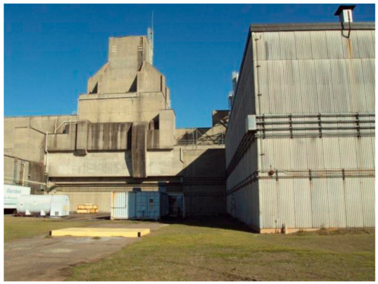
Figure 1.
Reactor building 105-C at the Savannah River Site.
To aid in the development of damage algorithms and to provide a more controlled study, an aged reinforced concrete block specimen cut from a similar reactor facility was maintained and monitored in the University of South Carolina Structures and Materials Laboratory for the majority of the project duration. This specimen was subjected to wet/dry cycling to accelerate the corrosion process. Electrochemical measurements were periodically recorded while acoustic emission was monitored continuously.
The activities undertaken and reported in this study represent a step toward the development of an acoustic emission based approach for the assessment of reinforced concrete structural systems through remote monitoring. To the authors’ knowledge, this research is the first of its kind to study the suitability of acoustic emission to monitor corrosion damage in the field while comparing the results to a test block from a similar structure tested in a controlled laboratory environment.
The study is divided into two main activities: (1) Remote acoustic emission monitoring and analysis of data collected at the 105-C Reactor Facility and (2) Accelerated corrosion testing to assess corrosion damage within an aged and reinforced concrete block supplied by SRNS at the University of South Carolina Structures and Materials laboratory.
2. AE Monitoring at the 105-C Reactor Facility
2.1. Acoustic Emission Sensing Systems
Two separate AE systems were utilized for remote monitoring at the 105-C Reactor Facility. These systems are referred to as a ‘wired’ AE system and a ‘wireless’ AE system. All acoustic emission system components and software were manufactured by Mistras Group, Inc. of Princeton Junction, New Jersey. The wired system utilized both R6I (peak resonance near 55 kHz) and WDI (relatively broadband) sensor types (calibration sheets for both sensor types are available in the manufacturer’s website). Both sensor types utilize integral pre-amplifiers within the stainless steel sensor housing. The resonant sensors are more sensitive to damage in reinforced concrete structures than the broadband sensors. However, the broadband sensors provide higher fidelity frequency data, which can be useful for data reduction and interpretation. The sensors were connected to a 16-channel DiSP acoustic emission data acquisition system that utilizes four high speed data acquisition boards specifically designed and manufactured for the acquisition and processing of acoustic emission data as well as specialized software (AEWin).
The wireless acoustic emission system (type 1284) includes 4 channels and utilizes low power PK6I acoustic emission sensors. These sensors are resonant in the vicinity of 55 kHz and utilize integrated preamplifiers within stainless steel housing. The sensors were connected to the 1284 system where preliminary processing of the data is performed. The data is transmitted through an antenna and is received through a base station module that is connected to a conventional laptop computer. Specialized wireless acoustic emission software (AEWin for Wireless) is used for controlling the data acquisition. This system was powered through solar panels connected to 12V DC batteries.
2.2. Installation of Acoustic Emission Systems
Prior to the installation at the Savannah River Site (SRS), the consistency of the sensor readings was checked using pencil lead breaks on an acrylic rod [24,25]. Six pencil lead breaks were performed for each sensor. An appropriate sensor response was demonstrated as the average amplitude response of a sensor type that was within ±6 dB of the average amplitude of the sensor group. A threshold of 40 dB was used for data collection. An analog filter was used to collect signals with a frequency between 1 kHz and 1 MHz. The waveform sampling rate was 1 million samples per second (MSPS) with 256 micro-seconds pre-trigger and 1 kilobyte length. Peak definition time (PDT), hit definition time (HDT), and hit lock-out time (HLT) were set to 200, 400, and 200 micro-seconds, respectively. Each AE system was connected to a cellular modem to allow for remote monitoring and each system was remotely controlled through appropriate software. This allowed for altering system settings and saving data at the University of South Carolina.
2.2.1. Crane Maintenance Area
The wired AE system was installed to monitor the activity in this area of building 105-C with ten sensors including five resonant sensors (type R6I) and five broadband sensors (type WDI). The sensors were installed at three different locations. The first location was near a column to roof interface (referred to as the ‘vertical column to roof interface location’). This area had been visually assessed by the Savannah River Nuclear Solutions/Savannah River National Laboratory (SRNS/SRNL) personnel and is known to have deteriorated in comparison to the majority of the structural system comprising the 105-C reactor building. Spalling occurred in this area in the recent past and ongoing corrosion activity was suspected. The area has undergone at least one repair activity in the past. A total of six sensors (three resonant and three broadband) were installed at this location, which is shown in Figure 2. The locations of the sensors were chosen to be near the exposed reinforcing bars showing visual signs of corrosion damage. The locations of the sensors with respect to the red dot shown in Figure 2 are provided in Table 1.
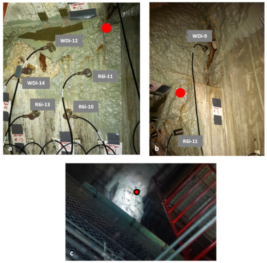
Figure 2.
Photographs of the crane maintenance area: (a) Main sensor grid, (b) close-up of sensor on side of column, and (c) view of main grid from the floor level (red dot is at corner).

Table 1.
Location of sensors shown in Figure 2.
The second location was chosen on a horizontal beam that forms the connection with the previously described column (referred to as the ‘horizontal beam location’). Two sensors (one resonant and one broadband) were installed at a distance of 12 inches below the beam to roof interface where signs of deterioration were visually observed (Figure 3a). The spacing between the sensors was 6 inches. The third location was chosen at an area where no signs of damage were observed (referred to as the ‘control location’). Two sensors (one resonant and one broadband) were installed at this location, which is shown in Figure 3b. The horizontal distance between the two sensors is 6 inches. The data collected from the control location was used to evaluate the effectiveness of data reduction approaches.
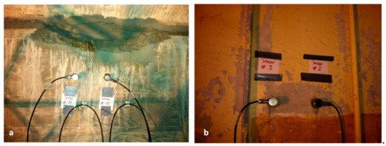
Figure 3.
Photograph of: (a) Horizontal beam location and (b) control location.
2.2.2. Top Floor Level
The wireless AE system was installed at the top floor level (also known as +48 level) to monitor a vertical crack that may penetrate an exterior wall, which is shown in Figure 4, using four resonant sensors (type PK6I). Sensor layout and spacing is also shown in the figure.
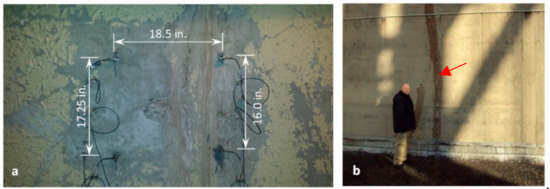
Figure 4.
Photographs at top floor level (+48 level): (a) Sensor grid from interior and (b) vertical crack from exterior.
2.3. Results and Discussion
2.3.1. Remote Monitoring at the Crane Maintenance Area
Remote monitoring at the Crane Maintenance Location was performed from 10 September 2014 (commencement of test) through 25 August 2015. A cellular connection was utilized to remotely operate the wired system. Data loss due to a power outage at the system occurred between 18 December 2014 and 20 January 2015. The raw data was analyzed and appropriate filters were used to reject data arising from signals not related to the initiation or the growth of cracks such as wave reflections. The filters are primarily parameter-based filters that were developed based on visual inspection of AE waveforms, which is similar to those described in ElBatanouny et al. (2014a). The first is a Duration-Amplitude filter (D-A), which is also referred to as a Swansong II type filter, while the second is a Rise Time-Amplitude filter (R-A), which is described in Table 2. Additional filters known as Duration and RMS filters were developed during this study to minimize electrical noise. The additional filters were developed based on data collected from the concrete block discussed in the following sections.
Table 2.
Data rejection limits.
Figure 5 and Figure 6 show the AE activity detected at the three monitored locations in the crane maintenance area for the resonant and broadband sensors, respectively. As shown in the figures, AE activity at the locations associated with visually observable damage (‘vertical column to roof interface location’ and ‘horizontal beam location’) was significantly higher than the AE activity at the control location. This indicates that the filters used were suitable for this application and also that intrinsic noise such as that potentially caused by electro-magnetic interference is not an obstacle for this application. The relatively high levels of AE activity indicate that damage (corrosion and related cracking) associated with the aging of reinforced concrete is progressing at the vertical column to roof interface and the horizontal beam locations.
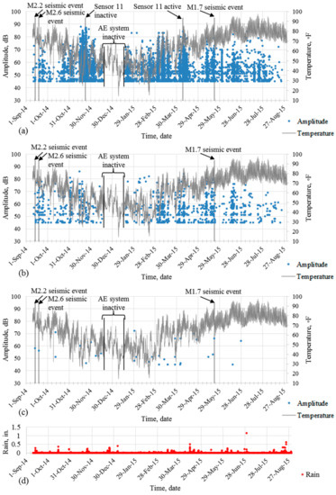
Figure 5.
Amplitude and temperature versus time for resonant sensors: (a) Vertical column to roof interface location, (b) horizontal beam location, (c) control location, and (d) rain versus time.
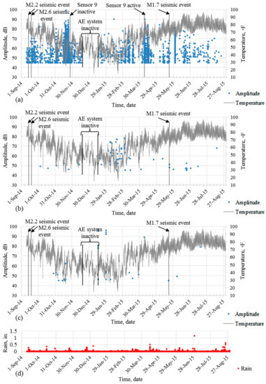
Figure 6.
Amplitude and temperature versus time for broadband sensors: (a) Vertical column to roof interface location, (b) horizontal beam location, (c) control location, and (d) rain versus time.
Rain and temperature data were provided by SRNL to investigate the effect of environmental conditions on AE activity. Seasonal temperature fluctuations affected the data more significantly than daily temperature fluctuations. This may be attributed to the low coefficient of thermal expansion of concrete, which causes volumetric changes to be associated with prolonged exposure to temperature differentials. As a general statement, increased AE activity was recorded when temperatures decreased during the winter months. Rain events were not as closely correlated to AE activity as were temperature fluctuations. However, associated moisture and repeated wet/dry cycling from rain events may lead to acceleration of the degradation process. During one of the site visits, remnants of a crack sealing material were found on the floor of the 105-C building, which indicates one potential source of moisture intrusion in this area.
The wired AE system was inactive between 18 December 2014 and 20 January 2015 due to a moisture-related event that adversely affected the laptop. Sensors corresponding to channels 9 and 11 (both at the vertical column to roof interface location) detached from the concrete surface on 27 November 2014 and 23 November 2014, respectively. Localized spalling that occurred at these locations during this time period is presumed to be the cause of the detachment. Both sensors were reattached on 8 April 2015.
Three seismic events occurred during the monitoring period: 14 September 2014 (M2.2), 19 September 2014 (M2.6), and 22 May 2015 (M1.96). Close inspection of data collected during this period did not reveal a correlation between these events and the AE data. Referring to the definition of acoustic emission (transient stress waves caused by a rapid release of energy within a material, [13], AE sensors would potentially be capable of detecting crack growth events caused by a seismic event provided the crack growth event or events that occurred within the range of sensitivity of the sensors. In the application at 105-C, the range of sensitivity for minor crack growth events (similar in energy to that caused by a pencil lead break) is in the range of 3 to 10 feet from each sensor. Due to the frequency range of AE sensors (30 kHz to 300 kHz), the sensors are not sensitive to global structural vibrations such as those potentially related to seismic activity.
2.3.2. Evaluation of Data at the Crane Maintenance Area
Figure 7a,b show the cumulative signal strength (abbreviated as CSS) at each monitored location for resonant and broadband sensors, respectively. Signal strength of an AE hit is a measure of the area under the recorded signal envelope (sometimes referred to as MARSE, Measured Area under the Rectified Signal Envelope) [13]. Higher levels of signal strength are associated with higher levels of energy release due to crack growth events.
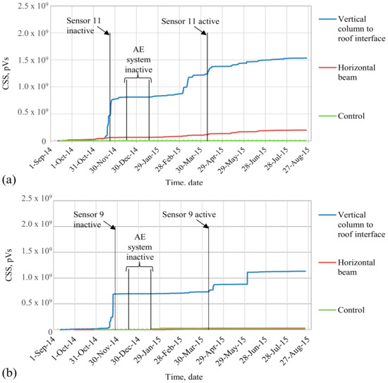
Figure 7.
Cumulative signal strength (CSS) of: (a) Resonant sensor and (b) broadband sensors.
While the signal strength of an AE hit is related to the intensity of damage growth at a particular instant in time, cumulative signal strength is related to increases in damage growth rates over a particular testing period. Rapid increases in the cumulative signal strength curve are related to rapid increases in damage growth. The relationship between rapid changes in the cumulative signal strength curve and damage growth has been utilized to assess damage in different structural systems [26] including reinforced concrete bridges [12] and corrosion damage in reinforced concrete laboratory specimens [2,3].
In both Figure 7a,b, it is apparent that sharp changes in the slope of cumulative signal strength that indicate sharp increases in damage progression related to the vertical column to roof interface location occurred in several different instances. For example, a sharp increase in damage growth is noticed at the end of November, between 4 March 2015 and 13 March 2015, and between 8 April 2015 and 15 April 2015. These sharp increases were noticed for both the resonant and broadband sensor types. As expected, the broadband sensors exhibit slightly lower values of cumulative signal strength due to the relatively low sensitivity of this sensor type.
The highest change of slope for resonant and broadband sensors at the vertical column to roof interface occurred at the end of November in 2014. This sudden increase in cumulative signal strength was accompanied by localized spalling of concrete, which may have caused the detachment of two sensors previously mentioned. This spalling supports the findings that significant damage occurred during this time period.
To allow for the comparison of AE activity from each sensor, the response of broadband sensors was normalized to that of resonant sensors. The normalization was determined based on the application of a simulated source [25] applied at both resonant and broadband sensor locations on the reactor concrete block. Pencil lead breaks (PLBs) were applied at different angles around a resonant sensor (0, 45, 90, 135, and 180 degrees) at distances of 3 inches and 6 inches in each direction. Three PLBs were applied at each distance. The CSS recorded from PLBs applied at each distance was calculated separately. The same procedure was repeated for a broadband sensor. The ratio of CSS detected from the resonant sensor to the CSS from the broadband sensor was calculated for the cases of 3 inches and 6 inches from the sensor. The average of the ratios achieved at the two distances was found to be approximately equal to 10. Thus, cumulative signal strength detected from WDI sensors was normalized using a factor of 10.
Figure 8a is a visual representation of the intensity of damage at each sensor location using a contour plot. The plot is based on cumulative signal strength results (units of pico-Volt seconds) where high cumulative signal strength is plotted in red, which indicates high damage while low cumulative signal strength is plotted in blue. This indicates lower damage. The contour plots show relative intensity of AE activity.
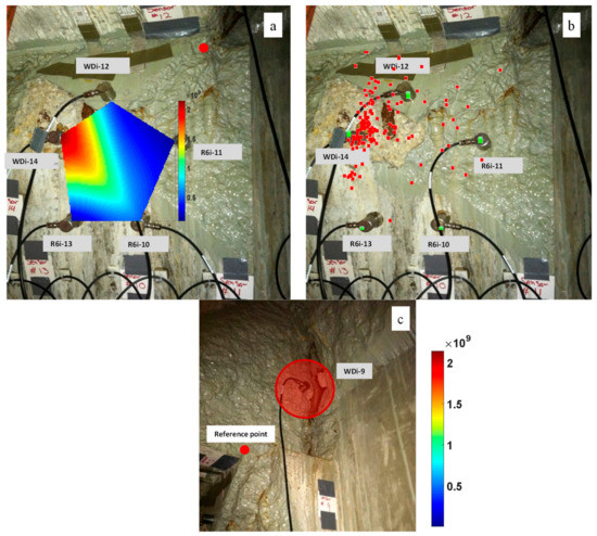
Figure 8.
Vertical column to roof interface: (a) Signal strength contour plot at elevation face sensors, (b) source location at elevation face sensors, and (c) signal strength contour plot at the side face sensor.
As seen in the plot, the highest normalized cumulative signal strength values were detected at the top left of the elevation face sensors and at sensor 9 at the side of the vertical column. The 2D source location results (for the data detected from the five sensors at the same plane) show that most AE events were also detected at the top left of the sensor grid, which suggests that damage is progressing at this location (Figure 8b). Figure 8c likewise indicates very high damage progression in the vicinity of sensor 9 with the highest value of normalized CSS detected at sensor 9.
Figure 9 shows similar contour plots at the horizontal beam and control locations. Similar to the vertical column to roof interface location, normalized data was used to generate the plot. The same contour scale seen in Figure 8 was used to generate the plots. As seen in Figure 9, lower damage occurred at the horizontal beam location (Figure 9a) and the control location (Figure 9b) when compared to vertical column-to-roof interface location.
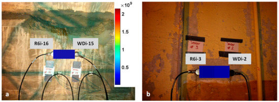
Figure 9.
Signal strength contour plot: (a) Horizontal beam location and (b) control location.
2.3.3. Damage Classification Using Acoustic Emission
To provide a means for interpretation of the data, Intensity Analysis graphs were developed at each AE monitoring location. The method was first introduced by Fowler and others [26] for the evaluation of fiber reinforced polymer vessels and is based entirely on signal strength. Intensity Analysis is a graphical method that differs from many other forms of acoustic emission assessments in the sense that it is focused on trends in the AE data as opposed to individual events. Intensity Analysis uses two parameters, which are both based on signal strength: (a) historic index (plotted on the horizontal axis) and (b) severity (plotted on the vertical axis).
Historic index and severity can be calculated using Equations (1) and (2) where N is the number of hits up to time (t), Soi is the signal strength of the i-th event, and K is an empirically derived factor that varies with the number of hits. The value of K has been previously selected in one case as: (a) N/A if N ≤ 50, (b) K = N − 30 if 51 ≤ N ≤ 200, (c) K = 0.85N if 201 ≤ N ≤ 500, and (d) K = N − 75 if N ≥ 501 [4].
Historic index, H(t), is a form of trend analysis that incorporates historical data in the current measurement. It is sensitive to changes of slope in cumulative signal strength versus time and compares the signal strength of the most recent hits to a value of cumulative hits. Severity, Sr, is defined as the average signal strength for the 50 hits with the highest numerical value of signal strength. The intensity analysis method has been widely used for the assessment of structural systems during load testing including reinforced concrete systems [12,27,28] and has been extended to the case of corrosion damage in pre-stressed concrete specimens [2,3,4,22].
By plotting the maximum historic index and severity values obtained over the duration of the test, an Intensity Analysis plot is generated. Due to the relationship between AE signal strength and damage growth, points that plot upward and to the right are associated with higher levels of damage.
Because Intensity Analysis (IA) uses historical information, an initial point on the Intensity Analysis plot must be chosen. This may be approached through visual inspection, numerical modeling, electrochemical measurements (in the case of corrosion damage), coring and petrographic examination, and other methods including suitable nondestructive evaluation techniques. Only a visual inspection was practical for the monitored locations within 105-C. Therefore, the initial point was chosen based on visual inspection.
The values of historic index and severity for the initial point were considered to account for pre-existing damage such that the historic index value at any time cannot be less than that for the initial point. For the severity, the distribution of the highest 50 signal strength values collected during the monitoring period in terms of their scattering from the mean value was used to develop the other 50 signal strength values with the same distribution but have a mean value equal to the severity of the initial point. Then the highest 50 numerical values from the collective set of 100 signal strengths, 50 from the monitoring period, and 50 developed from the initial point are used to calculate an updated severity value that takes into account the pre-existing condition.
Figure 10 and Figure 11 are plots of Intensity Analysis results from the period beginning 10 September 2014 and ending 25 August 2015 for data recorded from resonant and broadband sensors, respectively. For the majority of field applications, only resonant sensors would be utilized due to the increased sensitivity of this sensor type in comparison to broadband sensors. The use of resonant sensors, therefore, reduces the number of sensors needed for a given application. However, resonant sensors do not provide high fidelity representations of the frequency content in comparison to broadband sensors. One purpose of using the two different sensor types is to investigate the associated differences in the results. The limits of the Intensity Analysis chart were developed based on data from resonant sensors [2]. Thus, it is expected that data collected from broadband sensors may yield underestimated damage classification if the same limits are used.
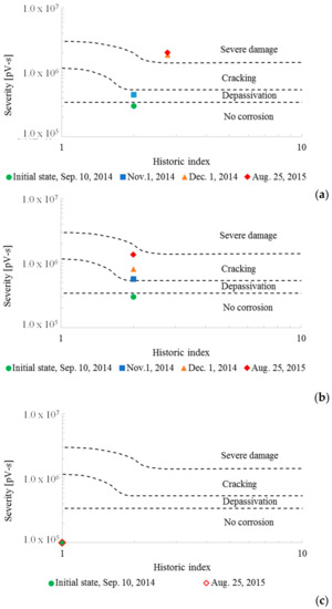
Figure 10.
Intensity Analysis results for resonant sensors: (a) roof to column interface, (b) horizontal beam location, and (c) control location.
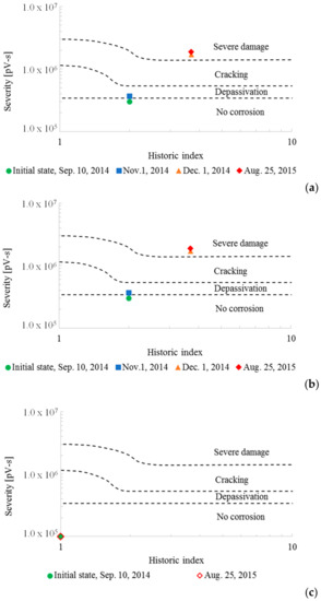
Figure 11.
Intensity Analysis results for broadband sensors: (a) roof to column interface, (b) horizontal beam location, and (c) control location.
The preliminary estimation of damage was based on visual inspection during the initial visit to 105-C and was located near the border between the ‘no damage’ and the ‘depassivation’ regions of the chart (severity = 300,000 and historic index = 2.0) for both the vertical column to roof interface location and the horizontal beam location. This assumed level of damage underestimated the actual condition of the structures since these areas are known to have ongoing corrosion damage. Ideally, this initial point would be established through a combination of methods including visual inspection and electrochemical methods. Electrochemical methods, however, were not collected during this part of the study. For the control location, no damage was assumed and, therefore, the initial point was located at the left corner in the ‘no corrosion’ region of the chart.
Acoustic emission activity during the monitoring period (approximately one year) at the vertical column to the roof interface location indicated a progression from the initial state to the severe damage state for both sensor types. It is noted that the results of IA after approximately 2 months of monitoring (1 November 2014) showed that corrosion is ongoing at this location. On 1 December 2014, Intensity Analysis results indicated that severe damage occurred. For monitoring over this relatively short duration, such a progression from the initial state to the ‘severe’ damage state is indicative of a relatively high level of ongoing damage growth in the monitored areas. For this plot, the term ‘cracking’ refers to micro-cracking that is generally non-visible while ‘severe damage’ refers to visible cracking that may be accompanied by spalling. This result is supported by the spalling that occurred at this location during the monitoring period.
Acoustic emission data from the resonant sensor and the broadband sensor at the horizontal beam location progressed from the initial state to the cracking state over the duration of the monitoring period. This result is also an indication of ongoing damage growth at this location when the relatively short monitoring period is considered. The broadband sensor results (Figure 11b) indicated less damage than the resonant sensor results (Figure 10b) especially during the first 3 months of monitoring. This can be attributed to the lower sensitivity of the broadband sensors.
In contrast to the roof interface location and the horizontal beam location, the intensity analysis results for the control location indicate no damage progression during the monitoring period and, therefore, the initial state and final state coincide (plot on top of one another) for the control location.
2.3.4. Remote Monitoring at +48 Level
A cellular connection was used to remotely operate the wireless acoustic emission data acquisition system. Data from the wireless system was collected between 9 September, 2014 (commencement of test) and 13 November 2014. Due to the loss of power from the solar power/battery system, 10 days of data were lost starting from 11 September 2014. The power was reconnected and the system continued to monitor the connection until 15 October 2014 when a thunderstorm caused a power outage and data was lost for another 13 days. The system continued to collect data afterwards until the data acquisition laptop was damaged on 13 November 2014. The damage was most likely due to moisture and was not repairable.
As described for the wired system data, the raw data was analyzed and appropriate data filters were used to separate meaningful data from spurious emissions. The limits of the data filters are shown in Table 2. Figure 12 shows acoustic emission activity in terms of amplitude versus time (showing both rain and temperature data) collected between 9 September 2014 and 13 November 2014 from the wireless acoustic emission system. This data set contains a significant number of hits with amplitude exceeding 80 dB. These hits are of relatively high amplitude and may be correlated to ongoing damage.
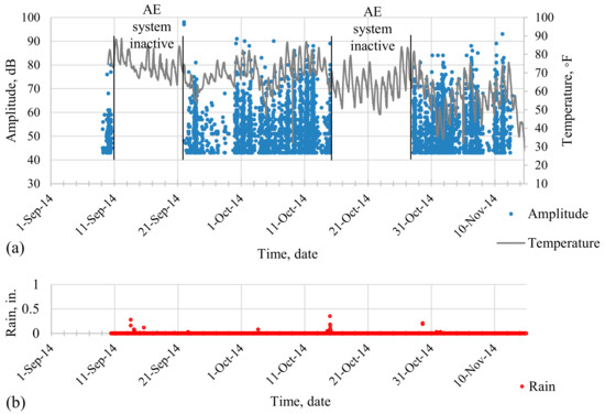
Figure 12.
(a) Amplitude and temperature versus time for four wireless sensors at the +48 level and (b) rain versus time.
One objective of monitoring this location was to assess whether the large vertical crack in the wall is still active. This vertical crack has a width between 0.125 and 0.25 inches with several small hairline cracks extending from it in the horizontal direction. Figure 13 plots the cumulative signal strength (units of pico-Volt seconds) versus time (days) for the collected signals over the monitoring period. An increasing trend in the acoustic emission activity is observed in the figures, which indicates that damage may be progressing at this location.
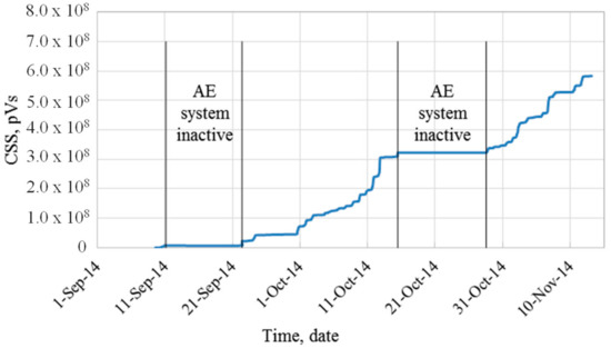
Figure 13.
Cumulative signal strength (pVs) versus time (days) for four wireless sensors at the +48 level.
To further investigate the trends in this data set, triangulation algorithms were used to investigate if AE events were generated from crack growth. Figure 14 shows the source location results from filtered acoustic emission data. In this figure, each red dot indicates a located acoustic emission event, which means that all four sensors received data with a specified time increment. The time increment was determined based on the characteristic wave speed of the structure, which was experimentally determined during the installation site visit, and the geometry of the sensor grid. Source location from raw data was inconclusive since it showed acoustic emission activity throughout the monitored area. The 6 acoustic emission events from the filtered data set were located in the vicinity of the vertical crack. These results imply that crack growth or friction between crack surfaces was ongoing in this area during the monitoring period.
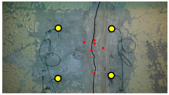
Figure 14.
Source location results at the +48 level. Red dots indicate located AE events.
3. Accelerated Corrosion Testing of the Reactor Concrete Block
3.1. Experimental Program
A reinforced concrete block was cut from the reactor facility with a length, width, and depth of 7 feet 4 inches, 3 feet, and 3 feet 4 inches, respectively. An accelerated corrosion test was conducted to corrode three different areas over the course of this study. Three concrete cores were drilled (3 inches in diameter and 9 inches in length) at three locations to create different concrete cover thickness for three vertical steel reinforcing bars adjacent to the cores (Figure 15). During the coring process, a transverse reinforcing bar was unavoidably cut at a depth of approximately 6 inches from the surface of the concrete test block specimen.
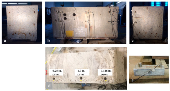
Figure 15.
Aged concrete block specimen: (a) Left side view, (b) front view, (c) right side view, (d) top view, and (e) control location.
The test was initiated by placing 3% NaCl solution in the drilled holes to a depth of 3 inches on 2 December 2014. The solution was maintained in the drilled holes for two months to ensure that chloride concentration reached a needed level for corrosion initiation [29,30]. Wet/dry cycles were then initiated (three days wet and four days dry) on 19 February 2015 to accelerate the corrosion process. A galvanic cell was created during the wet days by inserting a copper plate in the cored locations. Figure 15d shows the ‘as measured’ concrete cover after the cores were drilled.
The first location has a concrete cover of 0.25 inches and was monitored using three broadband sensors (WDI) and one resonant sensor (R15I) while the second location has a cover of 1.0 inch and was monitored using four resonant sensors (R6I). The third location has a cover of 0.125 inches and was monitored using eight resonant sensors (R6I). On 22 May 2015 one of the sensors at the 1.0 inch cover location was removed from the test block and, on 27 May 2015, it was placed on a small concrete specimen (control specimen) with dimensions of 3.0 inches × 3.0 inches × 11.25 inches. The control specimen is not reinforced and, therefore, is known not to have corrosion activity. Data collected from the control specimen was used to verify the efficiency of the data filters developed during the course of the project. Acoustic emission activity was recorded continuously throughout the test period.
Half-cell potential (HCP) and linear polarization resistance (LPR) measurements were recorded once a week with the objective of providing insight related to the corrosion process of targeted reinforcement locations. HCP method is described in ASTM C876 [31] and is traditionally employed to determine the likelihood of corrosion activity, which is described in Table 3. Linear polarization resistance (LPR) is a method used to measure polarization resistance (Rp), which can be used to calculate corrosion current (Icorr) and corrosion current density (icorr). These parameters can be used to estimate the corrosion rate (CR). Figure 16 shows a schematic of the test setup and acoustic emission sensor layout to monitor the corrosion process of the reinforcing bars. A schematic of the aged concrete block control specimen is also shown in this figure.
Table 3.
ASTM corrosion for Cu-CuSO4 reference electrode [31].
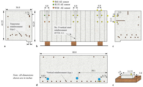
Figure 16.
Schematic of aged reactor concrete test block: (a) Left side view, (b) front view, (c) right side view, (d) top view, and (e) control location.
3.2. Results and Discussion
3.2.1. Electrochemical Measurements
Initial electrochemical measurements known as the half-cell potential were taken prior to the initiation of the conditioning period. These measurements indicated a passive state of steel reinforcement. The NaCl solution was then placed in the cored areas on 2 December 2015 and electrochemical readings were recorded weekly thereafter. As shown in Figure 17, three weeks after conditioning, half-cell potential values were observed to be more negative than −350 mV (referred to as the corrosion threshold) at all three locations. At the conclusion of the wet/dry cycles, half-cell potential readings indicated high corrosion risk in one of the three locations (0.25 inch cover location) and severe corrosion damage (more negative than −500 mV) in the other two locations (0.125 inch and 1.0 inch cover locations). The 1.0 inch cover location is known to have leakage associated with it since the NaCl solution drained continuously from this location from the commencement of the testing. While chloride diffusion is often assumed to be the primary initiator of corrosion damage, the presence of cracking in the concrete matrix may have a more profound effect on corrosion in some instances. The 0.125 inch cover and the 0.25 inch cover locations did not experience similar issues with leakage. The bottom of the hole at the 1.0 inch cover location was sealed with epoxy in the first week of April in 2015.
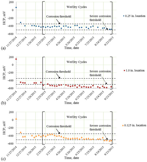
Figure 17.
Half-cell potential measurements at: (a) 0.25-inch concrete cover location, (b) 1.0-inch concrete cover location, and (c) 0.125-inch concrete cover locations.
Figure 18 shows linear polarization resistance results at the three locations with a logarithmic fit of the data points. The x-axis in Figure 18 represents the number of days after the solution was placed in the cored areas (initiated on 2 December 2014). The results indicate that all locations had relatively high corrosion rates since the polarization resistance was less than 100 ohms [4]. As seen in the figure, data was not collected between 24 December 2014 and 19 February 2015 (between 22 and 79 days) due to a malfunction with the potentiostat/galvanostat cable over that time period. This was addressed and the testing was resumed after 29 February, 2015. Since these readings are taken weekly over a time span of 300 days and due to the instantaneous nature of the readings, trends in the data set are more important than readings taken on a particular day. Therefore, trend lines with both upper and lower estimates are shown in the figures. A statistical method was used to eliminate outliers with low values to obtain the upper estimate and eliminate outliers with high values to obtain the lower estimate.
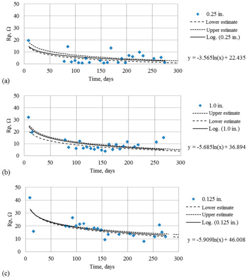
Figure 18.
Linear polarization resistance (LPR) measurements at: (a) 0.25-inch concrete cover location, (b) 1.0-inch concrete cover location, and (c) 0.125-inch concrete cover location.
3.2.2. Detection of Damage Using Acoustic Emission
Figure 19 shows the acoustic emission activity, in terms of amplitude versus time, recorded at locations monitored with resonant sensors (the 1.0 inch concrete cover location, the 0.125 inch concrete cover location, and the control location which was initiated on 27 May 2015). Figure 20 shows the acoustic emission activity recorded using broadband sensors at the 0.25 inch concrete cover location. The data shown in Figure 19 and Figure 20 was filtered using the data filters discussed in Table 2. An unusual amount of data that had characteristics related to electromagnetic interference was continually collected at the control location potentially due to damage in the sensor or cable during the removal and re-installation process. RMS and Duration data rejection limits were developed and were able to delete the majority of the false data without affecting data collected from other locations.
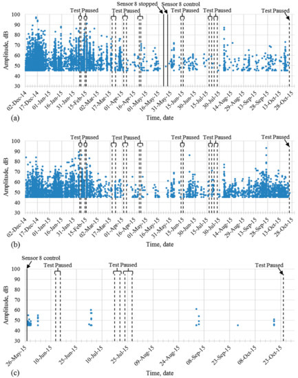
Figure 19.
AE data recorded from resonant sensors on the reactor concrete block specimen: (a) 1.0-inch concrete cover location, (b) 0.125-inch concrete cover location, and (c) control location.
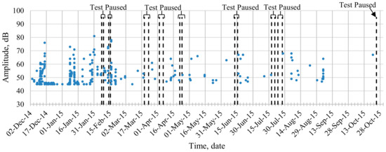
Figure 20.
AE data recorded from broadband sensors on the reactor concrete block specimen at the 0.25-inch concrete cover location.
As seen in Figure 19 and Figure 20, acoustic emission activity at the 1.0 inch concrete cover location and the 0.125 inch concrete cover location was higher than the acoustic emission activity at the 0.25 inch concrete cover location. This is attributed to the inherently higher sensitivity of the resonant sensors. It is noted that the rate of activity recorded at 1.0 inch concrete cover locations decreased during wet days after sealing the bottom of the hole.
To reduce the possibility of contaminating the acoustic emission data set with unrelated data generated from ongoing work in the University of South Carolina Structures and Materials Laboratory, the acoustic emission data acquisition system was intentionally paused on several occasions. Significant pauses in data acquisition are shown in the figures. A video camera monitoring the system was utilized to cross-verify and to aid in the development of data filters that are specific to ongoing work in the laboratory environment.
Figure 21 shows cumulative signal strength versus time at locations monitored using resonant sensors. It can be seen from this figure that cumulative signal strength increases rapidly at the beginning of the test, which corresponds to a period of rapid damage growth associated with corrosion initiation, enters a dormant period, and then increases slightly near the end of the testing period for the 1.0 inch and 0.125 inch locations. This trend in the data mirrors a trend noticed in the linear polarization resistance plots. The magnitude of the cumulative signal strength is greater for the 1.0-inch location when compared to the 0.125-inch location, which indicates increased acoustic emission activity and, therefore, increased damage growth at the 1.0-inch location. This is consistent with the electrochemical readings at this location and may be attributable to the presence of cracking in this location. The control location has minimal cumulative signal strength magnitude as would be expected. The relatively low cumulative signal strength magnitude at the control location demonstrates that unwanted acoustic emission data caused by ongoing laboratory activities in the vicinity of the test block specimen were minimized in the data sets.
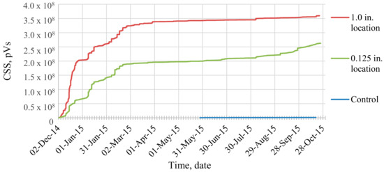
Figure 21.
Cumulative signal strength from resonant sensors on the aged concrete block specimen.
The broadband sensor data shows a similar trend of rapidly increasing damage early in the testing period, which is followed by a relatively dormant period at the 0.25 inch location. This is shown in Figure 22. The magnitude of cumulative signal strength from the broadband sensors is lower in comparison to the resonant sensors, which is expected due to the lower sensitivity of the broadband sensors.
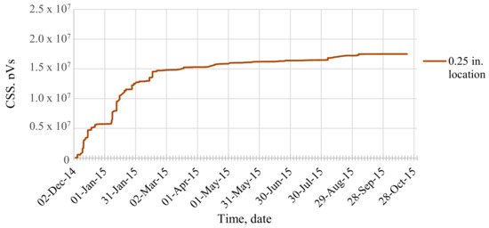
Figure 22.
Cumulative signal strength versus time from broadband sensors on the aged concrete block specimen.
Figure 23 and Figure 24 show the Intensity Analysis results calculated at each location. The estimation of initial damage for the aged concrete block specimen based on visual inspection and electrochemical results was located near the border between the ‘no damage’ region and the ‘depassivation’ region of the chart. For the control location, a lower initial damage state was used since no corrosion damage is expected in this specimen. AE activity from the resonant sensors at the 1.0-inch concrete cover location progressed from the initial state to the severe damage zone over the duration of the monitoring period. AE activity from the resonant sensors at the 0.125-inchconcrete cover location progressed from the initial state to the border of the cracking and severe damage zones. For the broadband sensors at the 0.25-inch concrete cover location, acoustic emission activity progressed from the initial state to the border of the cracking and severe damage zones.
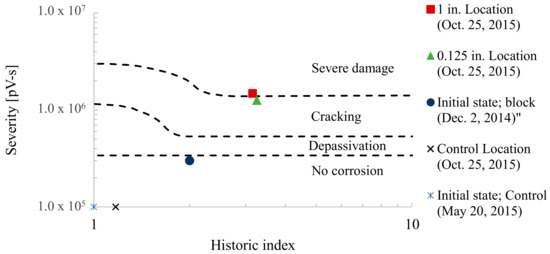
Figure 23.
Intensity Analysis for resonant sensors on the reactor concrete block specimen.
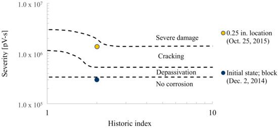
Figure 24.
Intensity Analysis for broadband sensors on the reactor concrete block specimen.
The above results are indicative of cracking in the concrete matrix due to corrosion activity at all three locations. As with the electrochemical measurements, the acoustic emission activity indicated that the most severe damage occurred at the 1.0-inch concrete cover location. As mentioned above, this location is affected by cracking as noticed through leakage of the NaCl solution at this location. While many degradation models for reinforced concrete are based on diffusion and, therefore, do not directly address the presence of cracking in the matrix. The effect of cracking in the matrix may, nonetheless, be significant. Similarly, many models assume a homogeneous concrete matrix. The lack of homogeneity in the concrete matrix for actual structures such as the concrete test block may also play a significant role in the results.
4. Summary and Conclusions
This investigation explores the implementation of acoustic emission monitoring as a remote structural assessment method. Acoustic emission systems were used to monitor corrosion damage and cracking in a decommissioned nuclear reactor facility as well as to monitor corrosion damage in a concrete block cut from the nuclear facility in laboratory conditions. The monitoring period in this study extended to approximately one year.
The study showed that long-term remote monitoring of ongoing damage in large scale existing structures is feasible using acoustic emission systems. For the wired system, AC power and cellular network connection are required for successful operation of the system. No major issues were encountered in terms of electromagnetic interference with the sensors, external noise and remote monitoring, and data transfer. The wireless system used has the potential to be used with solar power paired with cellular connections for the remote monitoring, which makes this approach well suited for long-term monitoring efforts. However, adequate protection to the electrical components is required especially in humid environments, which is illustrated by the failure of the data acquisition laptop due to moisture damage.
For the Reactor Building 105-C Crane Maintenance Area, the acoustic emission activity recorded at the ‘vertical column to roof interface location’ and ‘horizontal beam location’ varied throughout the monitoring period and tended to be associated with seasonal temperature fluctuations. The acoustic emission activity recorded at the ‘control location’ was significantly less when compared to the activity from the other two locations. Intensity Analysis was used to quantify the damage progression over the course of the monitoring period for both the broadband and resonant sensor types. The results of this method were in agreement with visually observed distress in the monitored locations. The assessed condition of the actively corroding areas progressed from the assumed condition of ‘no corrosion/approaching depassivation’ to ‘severe damage’ over the monitoring period while no change was observed in the state of the control location. It is noted that the assessed condition based on Intensity Analysis progressed to ‘cracking/severe damage’ within the first two months of monitoring. This shows the feasibility of this technique to successfully qualify active corrosion damage in structures in relatively small monitoring periods.
For the Reactor Building 105-C +48 level, the acoustic emission activity at the +48 location also varied with seasonal temperature fluctuations. This area contained a vertical crack in the exterior wall and it is possible that crack growth or friction between surfaces of this crack was the cause of much of the acoustic emission activity. Source location was carried out at this location and events were located in the vicinity of the vertical crack, which shows the feasibility of acoustic emission to detect and locate ongoing damage from cracking given that appropriate data filters are used.
For the Aged Concrete Test Block, both electrochemical results and acoustic emission cumulative signal strength versus time indicated that the corrosion activity occurred primarily during the first three to four months of conditioning and then continued at a reduced rate. Intensity Analysis based on the acquired data indicated that damage progressed from the assumed initial condition of ‘no corrosion/approaching depassivation’, determined based on electrochemical results upon arrival at the laboratory to ‘cracking/severe damage’ over the monitoring period for all three locations and for both sensor types. This Intensity Analysis result is similar to the one reported for the ‘vertical column-to-roof interface location’.
One of the main areas that hinder wide implementation of structural health monitoring systems is the large amounts of data that is collected and the subsequent effort needed to interpret and analyze this data in order to produce meaningful assessment of the condition of the structures. An important contribution of this study is that it proved the ability of well-developed data reduction and damage assessment algorithms to provide accurate evaluation of the condition of the structures. The results of the study showed that the developed filtering techniques along with the Intensity Analysis chart used for corrosion damage classification were able to successfully qualify the damage in the monitored areas. A method to account for pre-existing damage in the AE Intensity Analysis chart was also developed. These methods can be easily programmed and used to provide meaningful information to facility managers without the need for further assessment of large data sets. This can subsequently help in maintenance planning and prioritization especially in large scale and complex infrastructure systems.
Future research is needed to correlate acoustic emission data to electrochemical measurements especially in early corrosion stages, which will further enhance the outcome of monitoring. This will provide more insight regarding the progression of corrosion damage and can ultimately enable estimation of remaining service life.
Author Contributions
Conceptualization, M.A., M.E., K.D., M.S. and P.Z.; Methodology, P.Z., M.E. and M.A.; Validation, M.A. and M.E.; Formal Analysis, M.A.; Writing-Original Draft Preparation, M.A.; Writing-Review & Editing, M.E., P.Z., K.D. and M.S.; Supervision, P.Z.; Project Administration, P.Z. and M.S.; Funding Acquisition, P.Z., M.S., K.D. and M.E.
Acknowledgments
The authors would like to thank the support of Savannah River National Laboratory. Portions of this work are supported by the U.S. Department of Energy and Savannah River National Laboratory through SCUREF Funding. Portions of this work are supported by the U.S. Department of Commerce, National Institute of Standards and Technology (NIST), Technology Innovation Program (TIP), Cooperative Agreement 70NANB9H9007.
Conflicts of Interest
The authors declare no conflict of interest.
References
- Clifton, J.F. Predicting the Remaining Service Life of Concrete; National Institute of Standards and Technology: Gaithersburg, MD, USA, 1991. [Google Scholar]
- Mangual, J.; ElBatanouny, M.; Ziehl, P.; Matta, F. Acoustic-emission-based characterization of corrosion damage in cracked concrete with prestressing strand. ACI Mater. J. 2013, 110, 89–98. [Google Scholar]
- Mangual, J.; ElBatanouny, M.; Ziehl, P.; Matta, F. Corrosion damage quantification of prestressing strands using acoustic emission. J. Mater. Civ. Eng. 2013, 25, 1326–1334. [Google Scholar] [CrossRef]
- ElBatanouny, M.; Mangual, J.; Ziehl, P.; Matta, F. Early corrosion detection in prestressed concrete girders using acoustic emission. J. Mater. Civ. Eng. 2014, 26, 504–511. [Google Scholar] [CrossRef]
- Abdelrahman, M.; ElBatanouny, M.; Serrato, M.; Dixon, K.; Larosche, C.; Ziehl, P. Classification of alkali-silica reaction and corrosion distress using acoustic emission. AIP Conf. Proc. 2016, 1706, 140001. [Google Scholar]
- Fournier, B.; Berube, M.A.; Folliard, K.J.; Thomas, M. Report on the Diagnosis, Prognosis, and Mitigation of Alkali-Silica Reaction (ASR) in Transportation Structures; Transport Research International Documentation (TRID); Available online: https://trid.trb.org/view/1099043 (accessed on 30 June 2014).
- Abdelrahman, M.; ElBatanouny, M.; Ziehl, P.; Fasl, J.; Larosche, C.; Fraczek, J. Classification of alkali-silica reaction damage using acoustic emission: A proof-of-concept study. Constr. Build. Mater. 2015, 95, 406–413. [Google Scholar] [CrossRef]
- Braverman, J.I.; Xu, J.; Ellingwood, B.R.; Costantino, C.J.; Morante, R.J.; Hofmayer, C.H. Evaluation of the Seismic Design Criteria in ASCE/SEI Standard 43-05 for Application to Nuclear Power Plants; U.S. Nuclear Regulatory Commission: Washington, DC, USA, 2007; pp. 1–73. [Google Scholar]
- Kojima, F. Structural Health Monitoring of Nuclear Power Plants using Inverse Analysis in Measurements; Kobe University: Hyogo, Japan, 2009; Available online: http://www.research.kobe-u.ac.jp/csi-applmath/proc/workshopKobe/final/Section10.pdf (accessed on 31 December 2011).
- Abdelrahman, M.; ElBatanouny, M.; Ziehl, P. Acoustic emission based damage assessment method for prestressed concrete structures. Eng. Struct. 2014, 60, 258–264. [Google Scholar] [CrossRef]
- Ono, K. Application of Acoustic Emission for Structure Diagnosis; BazTech; Available online: http://yadda.icm.edu.pl/baztech/element/bwmeta1.element.baztech-article-BAR0-0060-0020 (accessed on 31 December 2011).
- Golaski, L.; Gebski, P.; Ono, K. Diagnostics of concrete bridges by acoustic emission. J. Acoust. Emiss. 2002, 20, 83–98. [Google Scholar]
- ASTM E1316-16a. Standard Terminology for Nondestructive Examinations; ASTM International: West Conshohocken, PA, USA, 2016; pp. 1–38. [Google Scholar]
- Pollock, A.A. Classical Wave Theory in Practical AE Testing. In Proceedings of the 8th International AE Symposium, Tokyo, Japan, 21–24 October 1986; pp. 708–721. [Google Scholar]
- Weng, M.S.; Dunn, S.E.; Hartt, W.H.; Brown, R.P. Application of Acoustic Emission to Detection of Reinforcing Steel Corrosion in Concrete. Corrosion 1982, 38, 9–14. [Google Scholar] [CrossRef]
- Dunn, S.E.; Young, J.D.; Hartt, W.H.; Brown, R.P. Acoustic emission characterization of corrosion induced damage in reinforced concrete. Corrosion 1984, 40, 339–343. [Google Scholar] [CrossRef]
- Zdunek, A.D.; Prine, D.W.; Li, Z.; Landis, E.; Shah, S. Early Detection of Steel Rebar Corrosion by Acoustic Emission Monitoring; NACE International: Houston, TX, USA, 1995. [Google Scholar]
- Li, Z.; Zudnek, A.; Landis, E.; Shah, S. Application of acoustic emission technique to detection of reinforcing steel corrosion in concrete. ACI Mater. J. 1998, 95, 68–76. [Google Scholar]
- Assouli, B.; Simescu, F.; Debicki, G.; Idrissi, H. Detection and identification of concrete cracking during corrosion of reinforced concrete by acoustic emission coupled to the electrochemical techniques. NDT E Int. 2005, 38, 682–689. [Google Scholar] [CrossRef]
- Ohtsu, M.; Tomoda, Y. Phenomenological model of corrosion on process in reinforced concrete identified by acoustic emission. ACI Mater. J. 2008, 105, 194–199. [Google Scholar]
- Di Benedetti, M.; Loreto, G.; Matta, F.; Nanni, A. Acoustic emission monitoring of reinforced concrete under accelerated corrosion. J. Mater. Civ. Eng. 2013, 25, 1022–1029. [Google Scholar] [CrossRef]
- Vélez, W.; Matta, F.; Ziehl, P. Acoustic emission monitoring of early corrosion in prestressed concrete piles. Struct. Control Health Monit. 2015, 22, 873–887. [Google Scholar] [CrossRef]
- Appalla, A.; ElBatanouny, M.; Velez, W.; Ziehl, P. Assessing corrosion damage in post-tensioned concrete structures using acoustic Emission. J. Mater. Civ. Eng. 2015, 28, 04015128. [Google Scholar] [CrossRef]
- ASTM E2075/E2075M-15. Standard Practice for Verifying the Consistency of AE-Sensor Response Using an Acrylic Rod; ASTM International: West Conshohocken, PA, USA, 2015; pp. 1–5. [Google Scholar]
- ASTM E2374-15. Standard Guide for Acoustic Emission System Performance Verification; ASTM International: West Conshohocken, PA, USA, 2015; pp. 1–5. [Google Scholar]
- Fowler, T.; Blessing, J.; Conlisk, P.; Swanson, T.L. The MONPAC system. J. Acoust. Emiss. 1989, 8, 1–8. [Google Scholar]
- Nair, A.; Cai, C.S. Acoustic emission monitoring of bridges: Review and case studies. Eng. Struct. 2010, 32, 1704–1714. [Google Scholar] [CrossRef]
- ElBatanouny, M.; Ziehl, P.; Larosche, A.; Mangual, J.; Matta, F.; Nanni, A. Acoustic emission monitoring for assessment of prestressed concrete beams. Constr. Build. Mater. 2014, 58, 46–53. [Google Scholar] [CrossRef]
- Nilsson, L.O.; Sandberg, P.; Poulsen, E.; Tang, L.; Andersen, A.; Frederiksen, J.M. HETEK, a System for Estimation of Chloride Ingress into Concrete Theoretical Background; Danish Technological Institute: Taastrup, Danmark, 2011. [Google Scholar]
- Vélez, W.; ElBatanouny, M.; Matta, F.; Ziehl, P.H. Assessment of Corrosion in Prestressed Concrete Piles in Marine Environment with Acoustic Emission; NACE International: Salt Lake City, UT, USA, 2012. [Google Scholar]
- ASTM C876-09. Standard Test Method for Half-Cell Potentials of Uncoated Reinforcing Steel in Concrete; ASTM International: West Conshohocken, PA, USA, 2009; pp. 1–8. [Google Scholar]


© 2018 by the authors. Licensee MDPI, Basel, Switzerland. This article is an open access article distributed under the terms and conditions of the Creative Commons Attribution (CC BY) license (http://creativecommons.org/licenses/by/4.0/).